
Static Attitude Determination Using Convolutional Neural Networks

 ,
,  , ,
, ,  ,
, 
Abstract
:1. Introduction
2. Background
2.1. Attitude Representations
2.2. Related Work
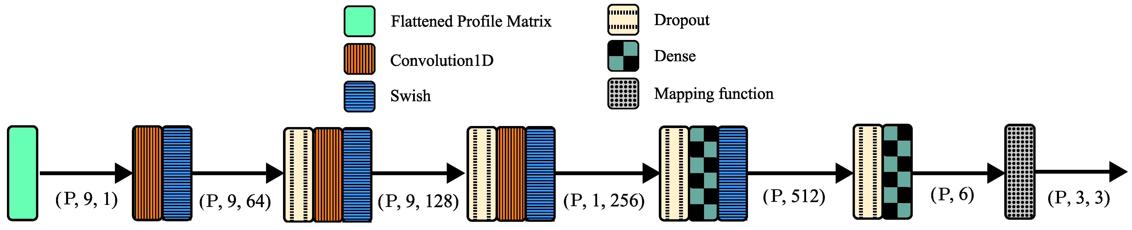
3. Methodology
3.1. Implementation Details
3.1.1. Dataset
3.1.2. Training
4. Results
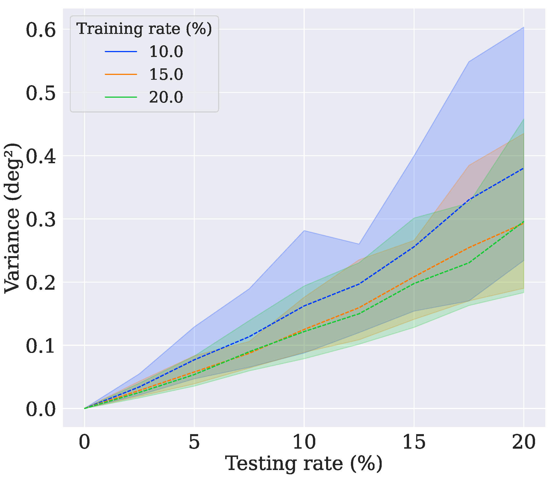
4.1. Model Training
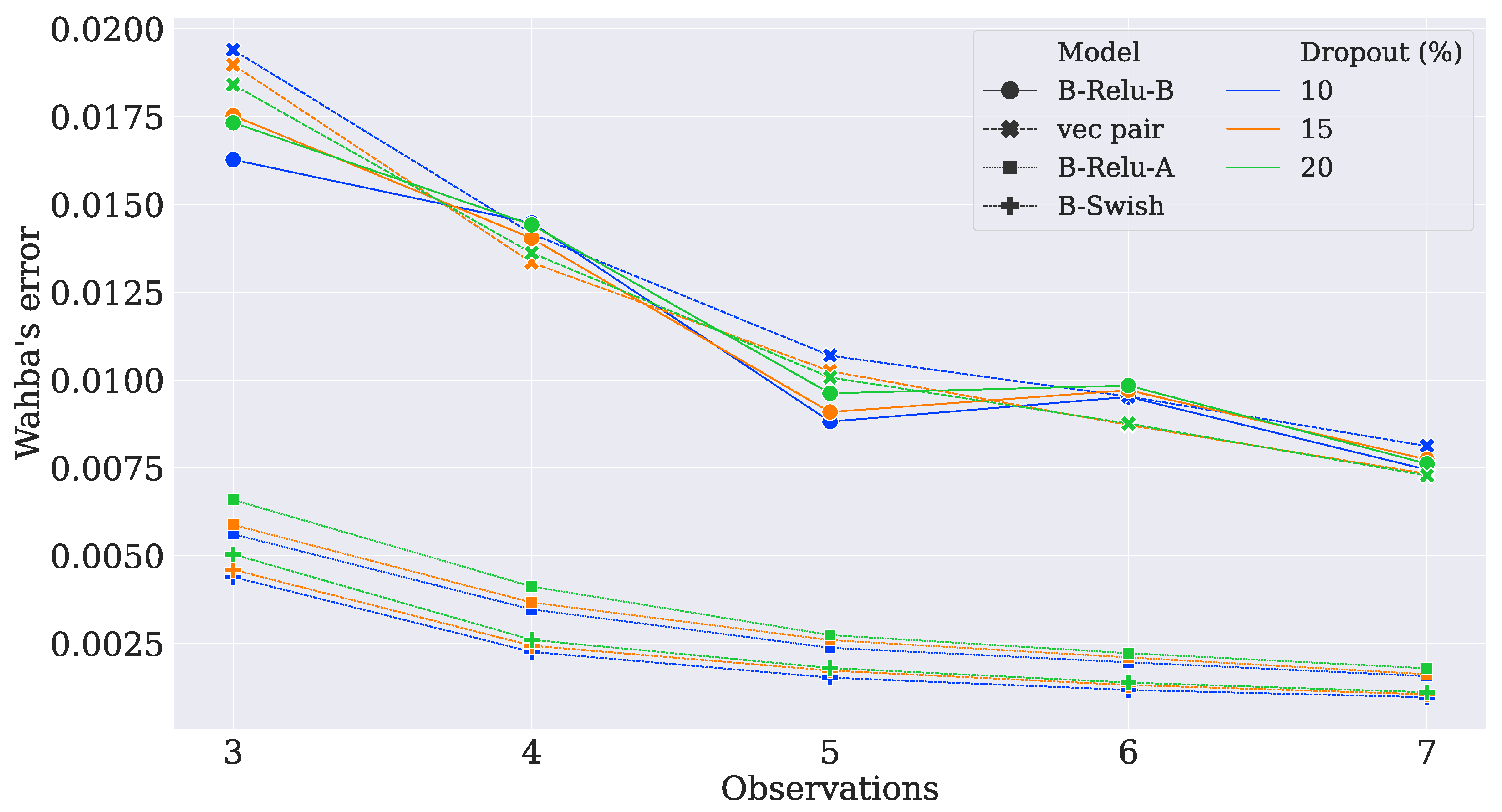
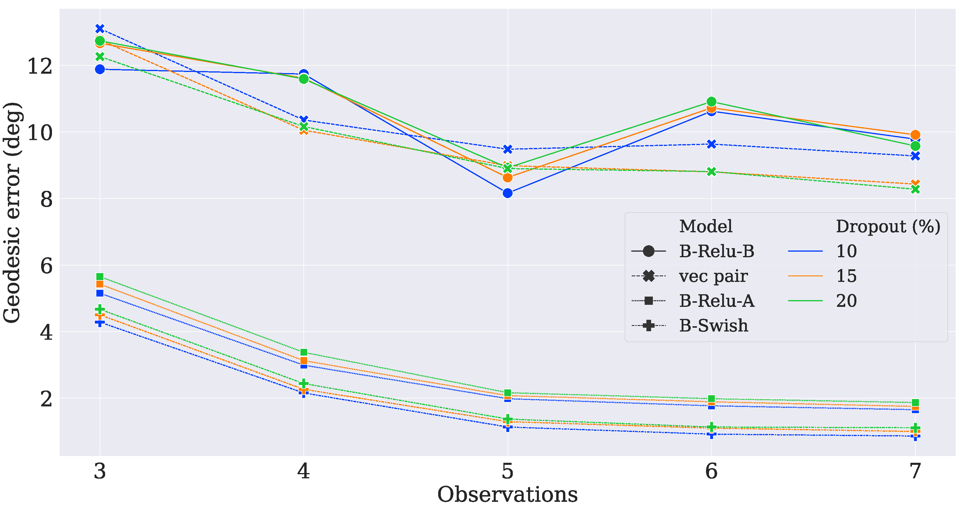
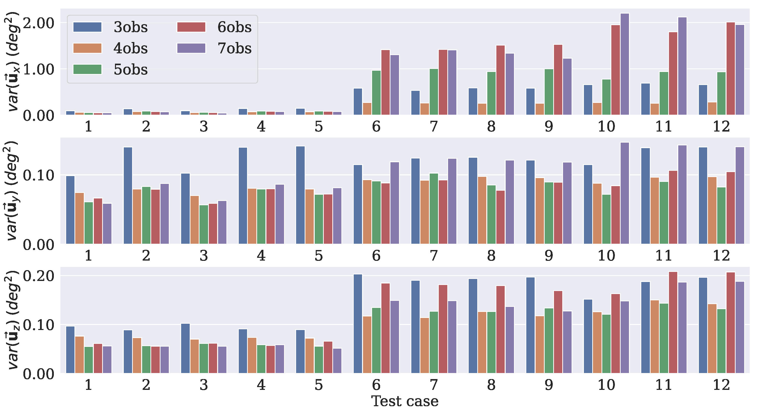
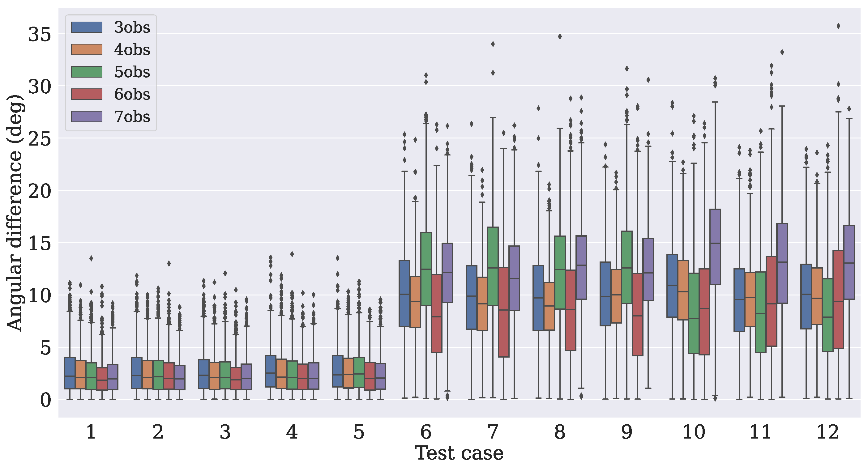
4.2. Model Choice
- Case 1
- In this case, there are three measurement vectors with measurement noise rad as follows:
- Case 2
- The same and vectors as those from Case 1 are used with measurement noise rad.
- Case 3
- The same three vectors from Case 1 are used, but the noise is increased to rad.
- Case 4
- The same as Case 2, but the the noise is increased to rad.
- Case 5
- Two reference vectors are used with measurement noise and rad as follows:
- Case 6
- In this case, there are three measurement vectors with measurement noise rad as follows:
- Case 7
- The same and vectors as those from Case 6 are used with measurement noise rad.
- Case 8
- The same three vectors as those from Case 6 are used, but the noise is increased to rad.
- Case 9
- The same as in Case 7, but the noise is increased to rad.
- Case 10
- Three reference vectors are used with measurement noise rad and rad as follows:
- Case 11
- The same and vectors as those from Case 10 are used with measurement noise rad and rad.
- Case 12
- The same and vectors as those from Case 10 are used with measurement noise rad and rad.
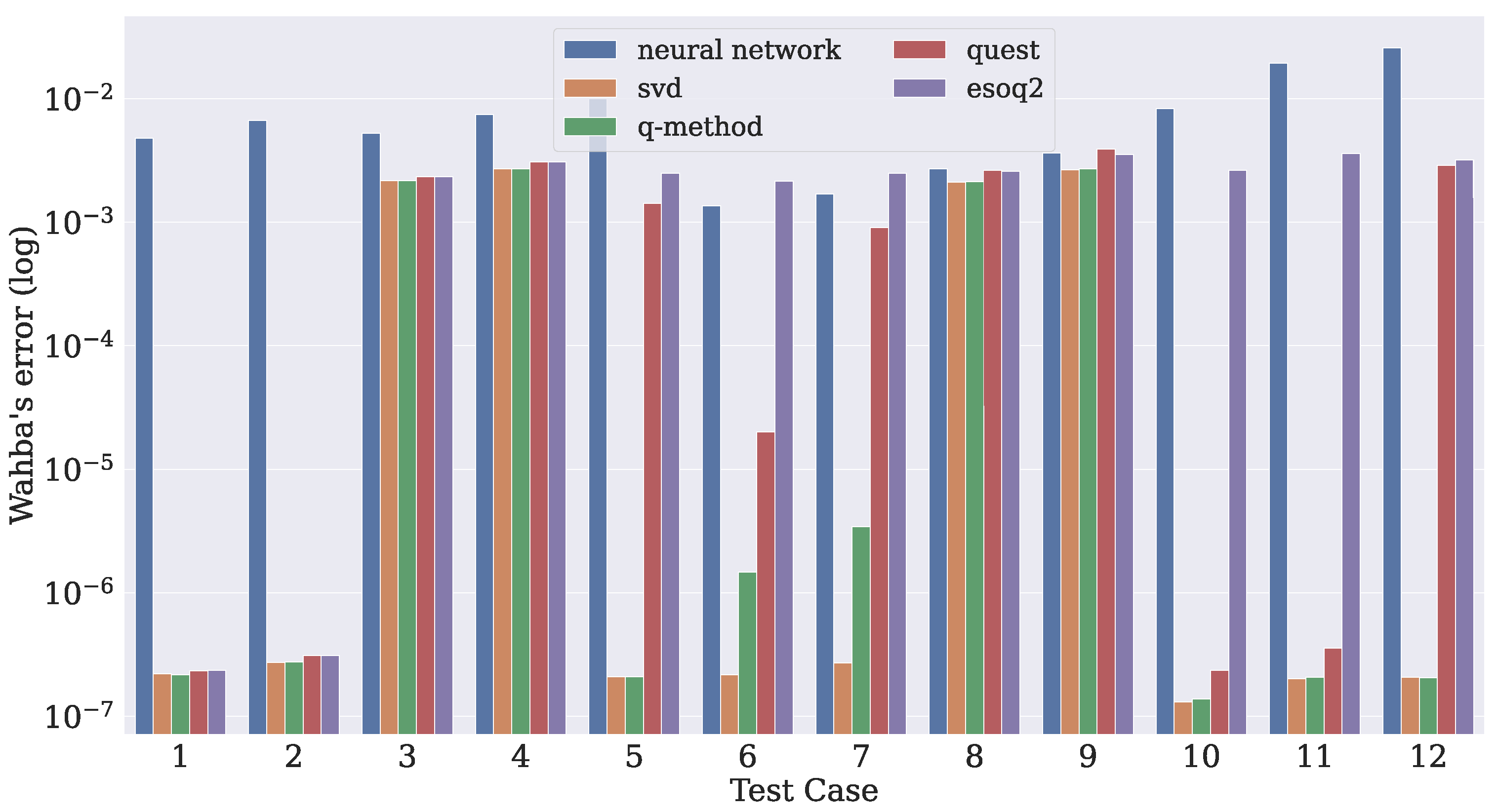
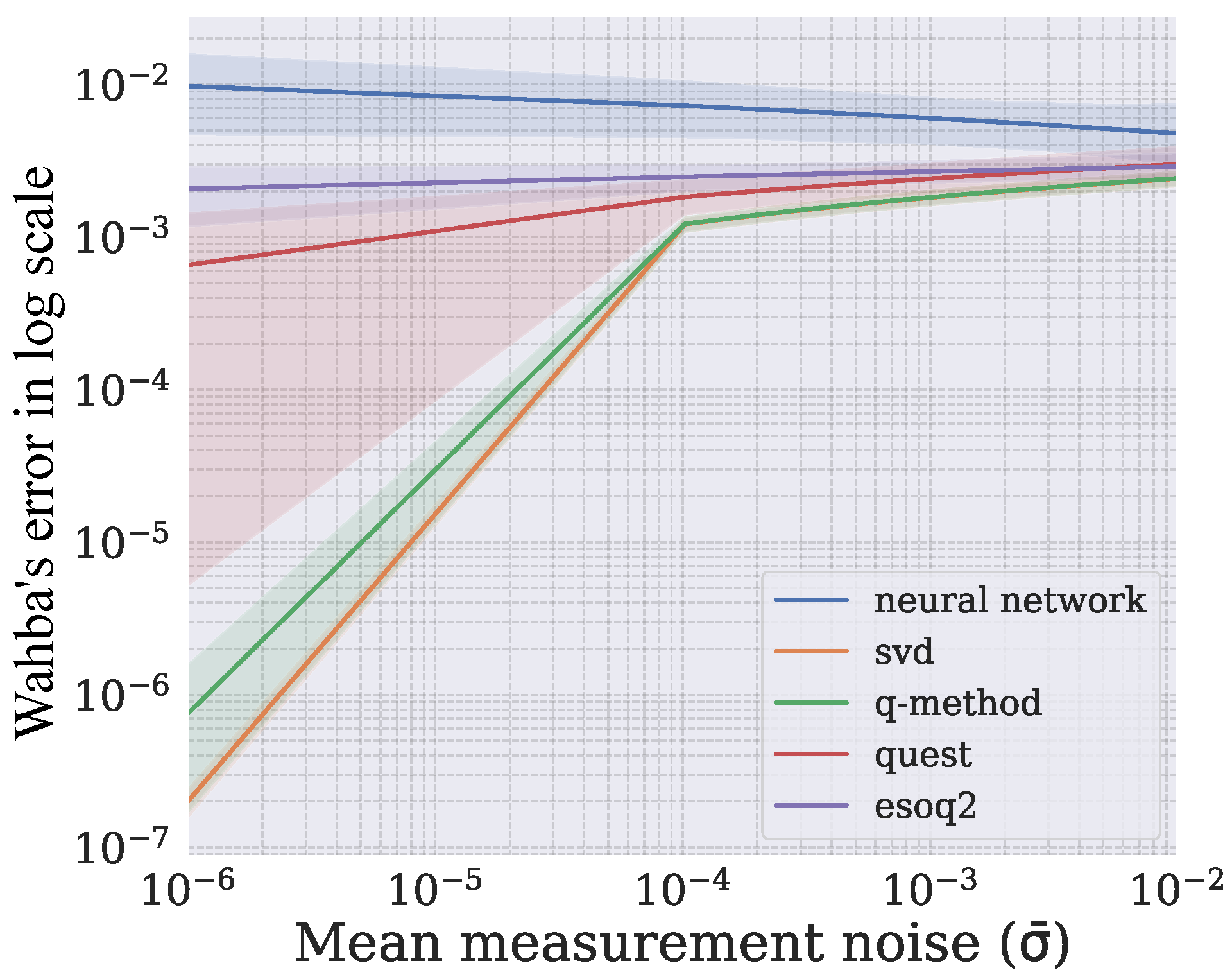
4.3. Comparison with Traditional Algorithms
5. Conclusions
Author Contributions
Funding
Institutional Review Board Statement
Informed Consent Statement
Data Availability Statement
Conflicts of Interest
References
- Le, T.T.; Le, T.S.; Chen, Y.R.; Vidal, J.; Lin, C.Y. 6D pose estimation with combined deep learning and 3D vision techniques for a fast and accurate object grasping. Robot. Auton. Syst. 2021, 141, 103775. [Google Scholar] [CrossRef]
- Wang, G.; Liu, X.; Han, S. A Method of Robot Base Frame Calibration by Using Dual Quaternion Algebra. IEEE Access 2018, 6, 74865–74873. [Google Scholar] [CrossRef]
- Suarez, A.; Heredia, G.; Ollero, A. Design of an Anthropomorphic, Compliant, and Lightweight Dual Arm for Aerial Manipulation. IEEE Access 2018, 6, 29173–29189. [Google Scholar] [CrossRef]
- Yin, P.; Ye, J.; Lin, G.; Wu, Q. Graph neural network for 6D object pose estimation. Knowl.-Based Syst. 2021, 218, 106839. [Google Scholar] [CrossRef]
- Tian, M.; Guan, B.; Xing, Z.; Fraundorfer, F. Efficient Ego-Motion Estimation for Multi-Camera Systems with Decoupled Rotation and Translation. IEEE Access 2020, 8, 153804–153814. [Google Scholar] [CrossRef]
- Cariow, A.; Cariowa, G.; Majorkowska-Mech, D. An algorithm for quaternion-based 3D rotation. Int. J. Appl. Math. Comput. Sci. 2020, 30, 149–160. [Google Scholar] [CrossRef]
- Wahba, G. A least squares estimate of satellite attitude. SIAM Rev. 1965, 7, 409. [Google Scholar] [CrossRef]
- Guo, C.; Li, F.; Tian, Z.; Guo, W.; Tan, S. Intelligent active fault-tolerant system for multi-source integrated navigation system based on deep neural network. Neural Comput. Appl. 2020, 32, 16857–16874. [Google Scholar] [CrossRef]
- Tan, T.N.; Khenchaf, A.; Comblet, F.; Franck, P.; Champeyroux, J.M.; Reichert, O. Robust-Extended Kalman Filter and Long Short-Term Memory Combination to Enhance the Quality of Single Point Positioning. Appl. Sci. 2020, 10, 4335. [Google Scholar] [CrossRef]
- Esfahani, M.A.; Wang, H.; Wu, K.; Yuan, S. OriNet: Robust 3-D Orientation Estimation With a Single Particular IMU. IEEE Robot. Autom. Lett. 2019, 5, 399–406. [Google Scholar] [CrossRef]
- Shuster, M.D. Approximate algorithms for fast optimal attitude computation. In Proceedings of the Guidance and Control Conference, Palo Alto, CA, USA, 7–9 August 1978; p. 1249. [Google Scholar]
- Shuster, M.D.; Oh, S.D. Three-axis attitude determination from vector observations. J. Guid. Control. 1981, 4, 70–77. [Google Scholar] [CrossRef]
- Markley, F.L. Attitude determination using vector observations and the singular value decomposition. J. Astronaut. Sci. 1988, 36, 245–258. [Google Scholar]
- Mortari, D. Second estimator of the optimal quaternion. J. Guid. Control. Dyn. 2000, 23, 885–888. [Google Scholar] [CrossRef]
- Davenport, P.B. A Vector Approach to the Algebra of Rotations with Applications; NASA Technical Note D-4696; NASA: Washington, DC, USA, 1968. [Google Scholar]
- Keat, J. Analysis of Least-Squares Attitude Determination Routine DOAOP (CSC/TM-77/6034); Technical Report CSC/TM-77/6034; Computer Sciences Corp.: Tysons, VA, USA, 1977. [Google Scholar]
- Spratling, B.B.; Mortari, D. A survey on star identification algorithms. Algorithms 2009, 2, 93–107. [Google Scholar] [CrossRef] [Green Version]
- Hashim, H.A. Attitude determination and estimation using vector observations: Review, challenges and comparative results. arXiv 2020, arXiv:2001.03787. [Google Scholar]
- Zhou, Y.; Barnes, C.; Lu, J.; Yang, J.; Li, H. On the continuity of rotation representations in neural networks. In Proceedings of the IEEE Conference on Computer Vision and Pattern Recognition, Long Beach, CA, USA, 16–20 June 2019; Volume 1, pp. 5745–5753. [Google Scholar]
- Xiang, Y.; Schmidt, T.; Narayanan, V.; Fox, D. Posecnn: A convolutional neural network for 6d object pose estimation in cluttered scenes. arXiv 2017, arXiv:1711.00199. [Google Scholar]
- Do, T.T.; Cai, M.; Pham, T.; Reid, I. Deep-6dpose: Recovering 6d object pose from a single rgb image. arXiv 2018, arXiv:1802.10367. [Google Scholar]
- Gao, G.; Lauri, M.; Zhang, J.; Frintrop, S. Occlusion resistant object rotation regression from point cloud segments. In Proceedings of the 15th European Conference on Computer Vision (ECCV), Munich, Germany, 8–14 September 2018; pp. 716–729. [Google Scholar]
- Park, J.M.; Yoo, Y.H.; Kim, U.H.; Lee, D.; Kim, J.H. D3PointNet: Dual-Level Defect Detection PointNet for Solder Paste Printer in Surface Mount Technology. IEEE Access 2020, 8, 140310–140322. [Google Scholar] [CrossRef]
- Yao, X.; Guo, J.; Hu, J.; Cao, Q. Using Deep Learning in Semantic Classification for Point Cloud Data. IEEE Access 2019, 7, 37121–37130. [Google Scholar] [CrossRef]
- Li, Y.; Bu, R.; Sun, M.; Wu, W.; Di, X.; Chen, B. Pointcnn: Convolution on x-transformed points. Adv. Neural Inf. Process. Syst. 2018, 31, 820–830. [Google Scholar]
- Jin, S.; Su, Y.; Gao, S.; Wu, F.; Ma, Q.; Xu, K.; Ma, Q.; Hu, T.; Liu, J.; Pang, S.; et al. Separating the Structural Components of Maize for Field Phenotyping Using Terrestrial LiDAR Data and Deep Convolutional Neural Networks. IEEE Trans. Geosci. Remote Sens. 2020, 58, 2644–2658. [Google Scholar] [CrossRef]
- Hu, P.; Kaashki, N.N.; Dadarlat, V.; Munteanu, A. Learning to Estimate the Body Shape Under Clothing From a Single 3-D Scan. IEEE Trans. Ind. Inform. 2021, 17, 3793–3802. [Google Scholar] [CrossRef]
- Peng, Y.; Chang, M.; Wang, Q.; Qian, Y.; Zhang, Y.; Wei, M.; Liao, X. Sparse-to-Dense Multi-Encoder Shape Completion of Unstructured Point Cloud. IEEE Access 2020, 8, 30969–30978. [Google Scholar] [CrossRef]
- Yu, Y.; Adu, K.; Tashi, N.; Anokye, P.; Wang, X.; Ayidzoe, M.A. RMAF: Relu-Memristor-Like Activation Function for Deep Learning. IEEE Access 2020, 8, 72727–72741. [Google Scholar] [CrossRef]
- Qian, L.; Hu, L.; Zhao, L.; Wang, T.; Jiang, R. Sequence-Dropout Block for Reducing Overfitting Problem in Image Classification. IEEE Access 2020, 8, 62830–62840. [Google Scholar] [CrossRef]
- Zhang, Q.H.; Ni, Y.Q. Improved Most Likely Heteroscedastic Gaussian Process Regression via Bayesian Residual Moment Estimator. IEEE Trans. Signal Process. 2020, 68, 3450–3460. [Google Scholar] [CrossRef]
- Mamo, T.; Wang, F.K. Long Short-Term Memory With Attention Mechanism for State of Charge Estimation of Lithium-Ion Batteries. IEEE Access 2020, 8, 94140–94151. [Google Scholar] [CrossRef]
- Xu, Z.; Xie, J.; Zhou, Z.; Zhao, J.; Xu, Z. Accurate Direct Strapdown Direction Cosine Algorithm. IEEE Trans. Aerosp. Electron. Syst. 2019, 55, 2045–2053. [Google Scholar] [CrossRef]
- Dytso, A.; Cardone, M.; Poor, H.V. On Estimating the Norm of a Gaussian Vector Under Additive White Gaussian Noise. IEEE Signal Process. Lett. 2019, 26, 1325–1329. [Google Scholar] [CrossRef]
- Stefenon, S.F.; Kasburg, C.; Nied, A.; Klaar, A.C.R.; Ferreira, F.C.S.; Branco, N.W. Hybrid deep learning for power generation forecasting in active solar trackers. IET Gener. Trans. Distrib. 2020, 14, 5667–5674. [Google Scholar] [CrossRef]
- Markley, F.L. Attitude Determination from Vector Observations: A Fast Optimal Matrix Algorithm. J. Astronaut. Sci. 1993, 41, 261–280. [Google Scholar]
- Franaszek, M.; Cheok, G.S. Orientation uncertainty characteristics of some pose measuring systems. Math. Probl. Eng. 2017, 2017, 2696108. [Google Scholar] [CrossRef] [PubMed] [Green Version]
- Curtis, W.D.; Janin, A.L.; Zikan, K. A note on averaging rotations. In Proceedings of the IEEE Virtual Reality Annual International Symposium, Seattle, WA, USA, 18–22 September 1993; pp. 377–385. [Google Scholar]
- Paiva, L.P.S.; de Melo, F.M.S.R.; Menezes Filho, R.; Vieira, L.A.; Oliveira, F. Error analysis for alignment in AHRS: QUEST and SAAM algorithms. An. Soc. Bras. Autom. 2020, 2. [Google Scholar] [CrossRef]
- Wu, J. Rigid 3-D Registration: A Simple Method Free of SVD and Eigendecomposition. IEEE Trans. Instrum. Meas. 2020, 69, 8288–8303. [Google Scholar] [CrossRef]


| Model | 3obs | 4obs | 5obs | 6obs | 7obs | ||||||||||
|---|---|---|---|---|---|---|---|---|---|---|---|---|---|---|---|
| Dropout Rate (%) | 10 | 15 | 20 | 10 | 15 | 20 | 10 | 15 | 20 | 10 | 15 | 20 | 10 | 15 | 20 |
| Case | |||||||||||||||
| 1 | −2.03 | −1.96 | −1.90 | −2.04 | −2.00 | −1.93 | −2.17 | −2.02 | −1.99 | −2.10 | −2.08 | −1.99 | −2.14 | −2.07 | −1.97 |
| 2 | −1.81 | −1.75 | −1.68 | −1.86 | −1.78 | −1.73 | −1.92 | −1.82 | −1.76 | −1.86 | −1.85 | −1.76 | −1.95 | −1.80 | −1.76 |
| 3 | −2.00 | −1.94 | −1.90 | −2.06 | −1.98 | −1.92 | −2.12 | −2.02 | −1.97 | −2.08 | −2.05 | −1.98 | −2.11 | −2.06 | −1.97 |
| 4 | −1.80 | −1.74 | −1.69 | −1.86 | −1.78 | −1.74 | −1.92 | −1.83 | −1.75 | −1.85 | −1.84 | −1.75 | −1.91 | −1.79 | −1.77 |
| 5 | −1.82 | −1.75 | −1.69 | −1.81 | −1.72 | −1.71 | −1.94 | −1.79 | −1.78 | −1.90 | −1.88 | −1.79 | −1.93 | −1.79 | −1.74 |
| 6 | −1.94 | −1.87 | −1.85 | −2.05 | −1.97 | −1.91 | −1.89 | −1.87 | −1.71 | −1.75 | −1.78 | −1.73 | −1.83 | −1.77 | −1.75 |
| 7 | −1.77 | −1.67 | −1.65 | −1.87 | −1.78 | −1.72 | −1.70 | −1.68 | −1.53 | −1.58 | −1.61 | −1.53 | −1.65 | −1.60 | −1.57 |
| 8 | −1.92 | −1.85 | −1.83 | −2.02 | −1.96 | −1.87 | −1.89 | −1.86 | −1.69 | −1.75 | −1.77 | −1.74 | −1.82 | −1.76 | −1.74 |
| 9 | −1.75 | −1.68 | −1.65 | −1.85 | −1.78 | −1.71 | −1.71 | −1.69 | −1.52 | −1.56 | −1.60 | −1.55 | −1.65 | −1.60 | −1.56 |
| 10 | −1.95 | −1.92 | −1.83 | −1.88 | −1.91 | −1.88 | −1.92 | −1.90 | −1.81 | −1.73 | −1.73 | −1.76 | −1.73 | −1.70 | −1.64 |
| 11 | −1.75 | −1.68 | −1.65 | −1.65 | −1.63 | −1.62 | −1.67 | −1.65 | −1.65 | −1.64 | −1.56 | −1.54 | −1.54 | −1.58 | −1.54 |
| 12 | −1.56 | −1.53 | −1.53 | −1.54 | −1.58 | −1.57 | −1.49 | −1.64 | −1.53 | −1.37 | −1.44 | −1.46 | −1.39 | −1.46 | −1.35 |
Publisher’s Note: MDPI stays neutral with regard to jurisdictional claims in published maps and institutional affiliations. |
© 2021 by the authors. Licensee MDPI, Basel, Switzerland. This article is an open access article distributed under the terms and conditions of the Creative Commons Attribution (CC BY) license (https://creativecommons.org/licenses/by/4.0/).
Share and Cite
dos Santos, G.H.; Seman, L.O.; Bezerra, E.A.; Leithardt, V.R.Q.; Mendes, A.S.; Stefenon, S.F. Static Attitude Determination Using Convolutional Neural Networks. Sensors 2021, 21, 6419. https://0-doi-org.brum.beds.ac.uk/10.3390/s21196419
dos Santos GH, Seman LO, Bezerra EA, Leithardt VRQ, Mendes AS, Stefenon SF. Static Attitude Determination Using Convolutional Neural Networks. Sensors. 2021; 21(19):6419. https://0-doi-org.brum.beds.ac.uk/10.3390/s21196419
Chicago/Turabian Styledos Santos, Guilherme Henrique, Laio Oriel Seman, Eduardo Augusto Bezerra, Valderi Reis Quietinho Leithardt, André Sales Mendes, and Stéfano Frizzo Stefenon. 2021. "Static Attitude Determination Using Convolutional Neural Networks" Sensors 21, no. 19: 6419. https://0-doi-org.brum.beds.ac.uk/10.3390/s21196419