Article

A Two-Step Feature Selection Radiomic Approach to Predict Molecular Outcomes in Breast Cancer

1
IRCCS SYNLAB SDN, Istituto di Ricerca Diagnostica e Nucleare, Via E. Gianturco 113, 80143 Naples, Italy
2
Institute for High Performance Computing and Networking, National Research Council of Italy (ICAR-CNR), Via P. Castellino 111, 80131 Naples, Italy
3
Bio Check Up S.r.l., Via Riviera di Chiaia 9a, 80122 Naples, Italy
4
Department of Advanced Biomedical Sciences, University of Naples Federico II, 80131 Naples, Italy
*
Authors to whom correspondence should be addressed.
Submission received: 28 October 2022 / Revised: 13 January 2023 / Accepted: 24 January 2023 / Published: 31 January 2023
(This article belongs to the Special Issue Intelligent Systems for Clinical Care and Remote Patient Monitoring)

Abstract

:
Breast Cancer (BC) is the most common cancer among women worldwide and is characterized by intra- and inter-tumor heterogeneity that strongly contributes towards its poor prognosis. The Estrogen Receptor (ER), Progesterone Receptor (PR), Human Epidermal Growth Factor Receptor 2 (HER2), and Ki67 antigen are the most examined markers depicting BC heterogeneity and have been shown to have a strong impact on BC prognosis. Radiomics can noninvasively predict BC heterogeneity through the quantitative evaluation of medical images, such as Magnetic Resonance Imaging (MRI), which has become increasingly important in the detection and characterization of BC. However, the lack of comprehensive BC datasets in terms of molecular outcomes and MRI modalities, and the absence of a general methodology to build and compare feature selection approaches and predictive models, limit the routine use of radiomics in the BC clinical practice. In this work, a new radiomic approach based on a two-step feature selection process was proposed to build predictors for ER, PR, HER2, and Ki67 markers. An in-house dataset was used, containing 92 multiparametric MRIs of patients with histologically proven BC and all four relevant biomarkers available. Thousands of radiomic features were extracted from post-contrast and subtracted Dynamic Contrast-Enanched (DCE) MRI images, Apparent Diffusion Coefficient (ADC) maps, and T2-weighted (T2) images. The two-step feature selection approach was used to identify significant radiomic features properly and then to build the final prediction models. They showed remarkable results in terms of F1-score for all the biomarkers: 84%, 63%, 90%, and 72% for ER, HER2, Ki67, and PR, respectively. When possible, the models were validated on the TCGA/TCIA Breast Cancer dataset, returning promising results (F1-score = 88% for the ER+/ER− classification task). The developed approach efficiently characterized BC heterogeneity according to the examined molecular biomarkers.

1. Introduction

Breast Cancer (BC) is the most commonly diagnosed cancer type in the world. The most recent global cancer statistics estimate that there are about 2.3 million incident BC cases and that the disease is the leading cause of cancer mortality in women worldwide [1]. Currently, radiographic evaluation followed by a histological confirmation of malignancy on biopsy samples is used to make the early diagnosis of BC [2,3]. Although this method allows practitioners to safely and effectively characterize the molecular changes in breast tissue, it has intrinsic drawbacks because of the accessibility and heterogeneity of the tumors and the risks associated with the bioptic process [4].
In particular, it is well-known that the heterogeneity of BC, which also depends on the temporal variation, may lead to the failure of cancer treatments and poor prognoses [5].
The identification of numerous biomarkers through tissue biopsy or medical imaging is necessary for assessing heterogeneity at early diagnosis, with the correct classification of the tumor genotype being of fundamental importance for the clinical management of this pathology [6]. However, differently from imaging, the risks of invasive procedures, focal sampling errors, and tumoral characteristics (such as small size, location, or heterogeneous necrosis) represent relevant drawbacks associated with biopsies. In this perspective, radiomic techniques may notably support the non-invasive management of BC [7].
Radiomics was defined as “the high-throughput extraction of large amounts of image features from radiographic images” [8]. It could be used to analyze both temporal and spatial BC heterogeneities through the quantitative evaluation of the radiologic images. Recent developments in radiomics analysis showed the potential to retrieve useful incremental information from standard imaging data in a non-invasive way.
Radiomics can be successfully applied to both morphological (such as T2-weighted—T2—images) and functional magnetic resonance images (MRI) (such as dynamic contrast-enhanced (DCE) and diffusion-weighted imaging (DWI)) to predict histological outcomes in BC [9,10].
MRI is the reference imaging modality for soft tissue characterization, with functional techniques such as DCE-MRI and DWI greatly supporting the characterization of the anatomic and functional properties of BC [11,12]. In particular, MRI radiomics has been used to predict malignancy, molecular subtypes, complete pathological response to neoadjuvant chemotherapy, and metastasis in BC. However, both diagnostic and prognostic outcomes depend on the underlying biological characteristics of BC.
The accurate examination of BC biology is fundamental since each BC is characterized by a unique biological and genetic profile, thus corresponding to a wide range of prognoses and therapeutic options. Different molecular profiles, proliferative rates, tumor receptors, and grades define subtypes. The Estrogen Receptor (ER), Progesterone Receptor (PR), Human Epidermal Growth Factor Receptor 2 (HER2), and Ki67 antigen are the four biomarkers routinely examined in BC biopsies and excision specimens due to their potential impact on heterogeneity prognosis and clinical therapy. HER2-positive (HER2+) breast cancers are more aggressive and show a poorer prognosis than HER2-negative (HER2−) cancers. Positive hormonal receptor status, such as in ER-positive (ER+) and PR-positive (PR+) tumors, presents lower risk of mortality than ER-negative (ER−) and/or PR-negative (PR−) diseases. Ki67 is a proliferative index of BC, and a high Ki67 level is associated with an elevated relapse rate and worse survival [13].
There is a growing scientific production exploring different radiomic approaches to predict molecular outcomes of BC on MRI datasets [14,15,16,17,18,19,20]. Nevertheless, a common drawback affecting the largest part of these works was related to the absence of comprehensive sets of molecular markers and MRI modalities that would allow for an effective comparison of different models and feature selection approaches [9]. For instance, The Cancer Genome Atlas BReast invasive CArcinoma (TCGA-BRCA) dataset [21], collected by the TCGA/TCIA project, despite its limited size, still represents the largest publicly available set of breast MRI providing also clinical, pathological, and genomic data. However, TCGA-BRCA lacks information on the Ki67 molecular marker and does not include the DWI sequence.
This work aimed to develop a new radiomic approach based on a two-step feature selection process to predict the most routinely examined BC biomarkers (ER, PR, HER2, Ki67) and compare the prediction models’ performances in different settings. It exploited a comprehensive dataset that includes multiparametric MRI (mpMRI) images from morphological T2, functional DCE-MRI images, and Apparent Diffusion Coefficient (ADC) maps from DWI, as well as all four relevant molecular markers for BC management.

2. Materials and Methods

2.1. Study Design

The goal of the proposed methodology was to build robust predictors for the four biomarkers commonly used in BC molecular profiling. Two comprehensive datasets were exploited: the MOLIM ONCO BRAIN dataset (DS M ) for model development and the TCGA-BRCA (DS T ) for model validation. Both included: (i) mpMRI preoperative images of BC patients (both functional and morphological sequences), (ii) clinical information related to at least three biomarkers (ER, PR, HER2), and (iii) BC tumour segmentations. Figure 1 shows the steps of the radiomic pipeline used to carry out the model development and validation: mpMRI images acquisition (Section 2.3), tumor segmentation (Section 2.4), radiomic feature extraction (Section 2.5), a two-step feature selection and classification (Section 2.6), and best model selection and validation using an external dataset (Section 2.7).

2.2. Patients

The patient cohort included two datasets of BC patients. For the DS M , 92 MRI pre-operative examinations of patients with BC (93 lesions) were collected from February 2017 to February 2020 and retrospectively evaluated. Inclusion criteria were the following: (1) age >18 years and (2) patients with histologically proven BC. Patients were excluded if the histological report was unavailable and the MRI images were significantly affected by motion artifacts. All patient information was de-identified before the data were stored in the collection of BCU Imaging Biobank [22]. The study was approved by the Ethical Committee IRCCS Pascale (Prot. 12/19 OSS SDN), and written informed consent was obtained from all participants.
The DS T was used to perform model validation. It included 164 MRI studies (Digiatl Imaging and COmmunications in Medicine—DICOM—format, 88.1 GB) of 139 Breast Cancer patients from several American hospitals and clinics. The clinical, genetic, and pathological data were acquired from the Genomic Data Commons Data Portal [23]. To reduce potential image acquisition variation, only breast MRI studies that were similar in acquisition and technique (namely, MRIs that were acquired on a 1.5 T magnet strength using GE (GE Medical Systems, Milwaukee, WI, USA) scanners and protocols) were analyzed. This selection procedure resulted in a total of 93 patients. For these cases, tumor segmentations were available in binary format [24]. One subject with missing DCE images and one with missing genotyping data were excluded from the study. Finally, the DS T consisted of 91 BC patients. The images and segmentations were downloaded and converted in NIfTI (Neuroimaging Informatics Technology Initiative) format.

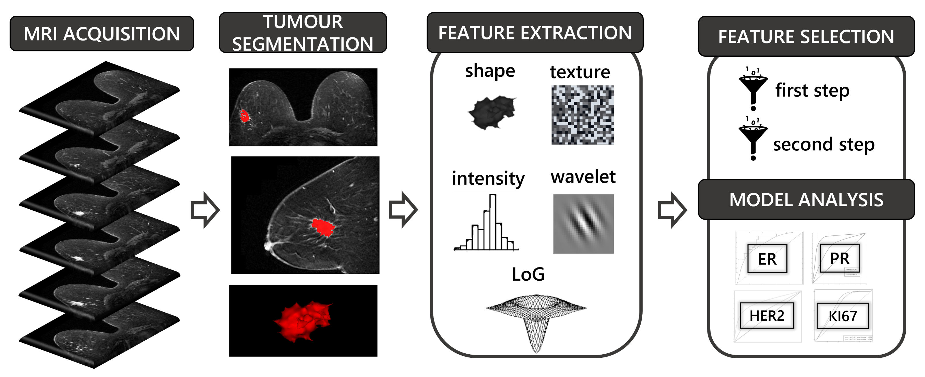
2.3. MRI Acquisition

MRI examinations of the DS M were performed using a 3 T Biograph mMR (Siemens Healthcare, Erlangen, Germany) with a dedicated breast surface coil. T2 Turbo spin-echo (TSE T2) sequence was acquired on an axial plane before contrast-agent injection, and DWI with b values of 50, 500, and 800 s/mm 2 was acquired on the axial plane with their corresponding ADC maps. DCE-MRI studies were obtained with intravenous administration of paramagnetic contrast agent (Prohance, Bracco Imaging, Italy) 0.3 mmol/kg, a flow rate of 3.5 mL/s, injected after six pre-contrast transaxial T1 Vibe with flip angles of 2 , 5 , 8 , 12 ,15 , and 20°, followed by a T1 Vibe axial dynamic (TR/TE = 5.47/1.75) with 60 measurements over a 10 min period and a temporal resolution of 9.6 s. Subtracted DCE images (SUB) were obtained automatically by subtracting pre-contrast images from the post-contrast (PC) images. Finally, an axial high-resolution T1 Vibe with fat suppression (HR Vibe T1-w fat sat) was acquired. Technical details of MRI sequences are shown in Table 1.

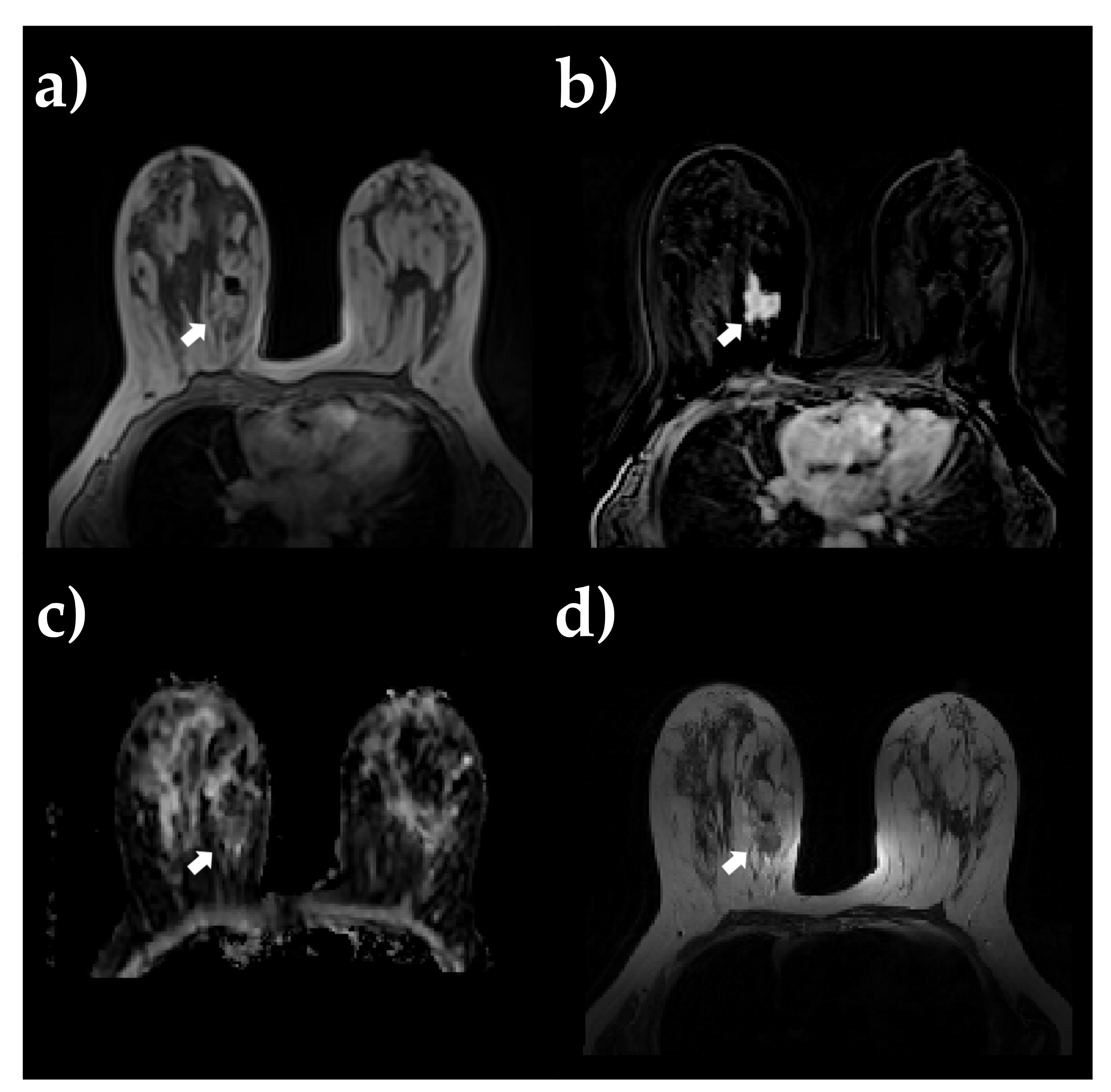
2.4. Image Processing and 3D ROI Segmentation

ADC images were non-rigidly coregistered on SUB PC DCE-MRI images using Elastix software (v4.9.0) to correct for typical spatial distortion arising from DWI acquisition. T2 images were all resliced on DCE-MRI images. Lesion segmentation was performed on SUB DCE images by an experienced radiologist using an in-house developed software for region labeling. During the segmentation procedure, the radiologist was blinded to both the histological results and all clinical information relative to the retrospective breast mpMRI images. The delineated ROIs were then copied and pasted into the PC DCE-MRI, registered ADC, and resliced T2 images (refer to Figure 2 for an example of primary BC lesion). Before radiomic feature extraction, normalization was applied on T2 and PC image intensities. Specifically, intensities were normalized by centering them at their respective mean value with a standard deviation of all grey values in the original image [25].

2.5. Feature Extraction

The extraction of radiomic features from 3D Regions of Interest (ROIs) on DCE-MRI subtraction series with the highest mean signal intensity within the ROI [26,27,28], PC DCE-MRI, registered ADC, and resliced T2 images was performed using the open source PyRadiomics package [29]. The obtained features can be classified into five classes: (i) shape features (n = 14); (ii) first-order features (n = 18); (iii) 73 s-order textural statistics including grey-level co-occurrence matrix (GLCM) (n = 24), grey-level run length matrix (GLRLM) (n = 16), grey-level size zone matrix (GLSZM) (n = 16), neighboring grey tone difference matrix (NGTDM) (n = 5), and grey-level dependence matrix (GLDM) (n = 14); 1092 transformed first-order and textural features including (iv) 728 wavelet features in frequency channels LHL, LLH, HHH, HLH, HLL, HHL, LHH, and LLL, where L and H are low- and high-pass filters, respectively; and (v) 364 Laplacian of Gaussian filtered features with sigma ranging from 2.0 to 5.0, with a step size = 1.

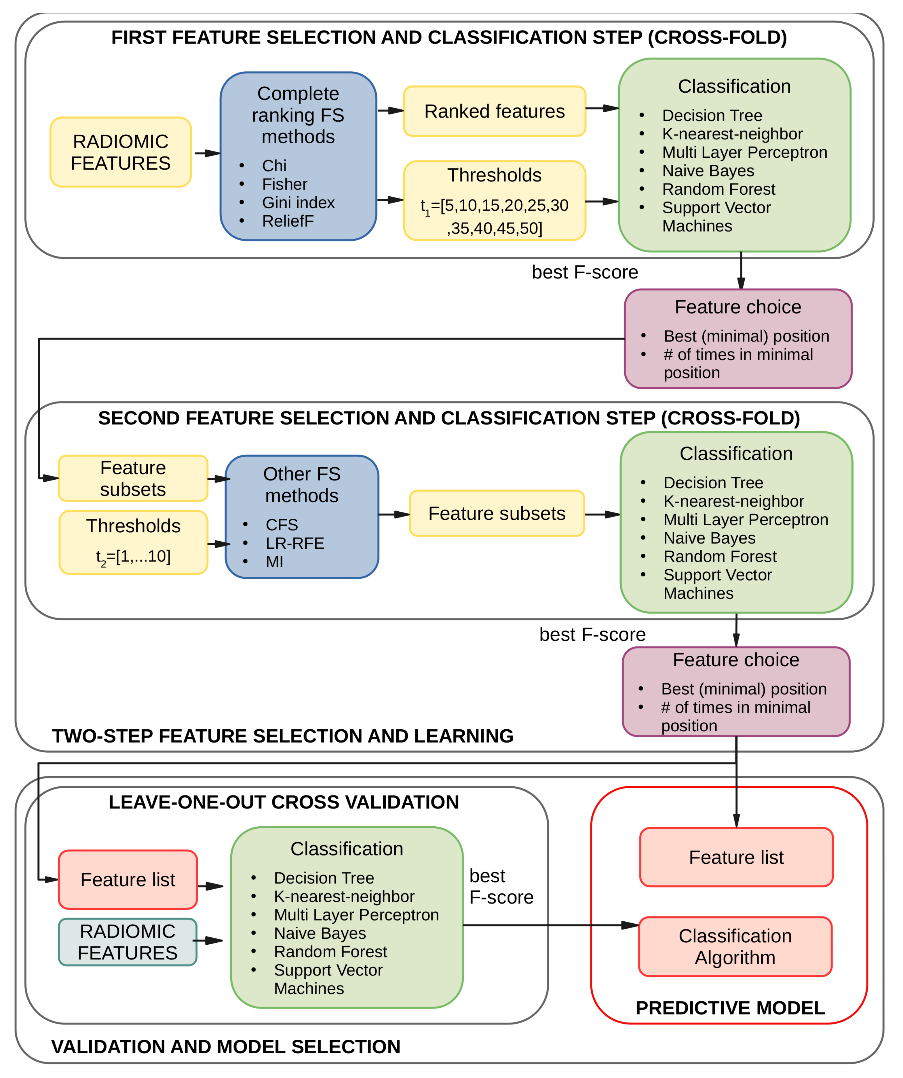
2.6. Two-Step Feature Selection and Learning

Since the number of extracted radiomics features was very high, using all of them for the classification step was generally ineffective because these features are redundant and highly correlated. Moreover, when the number of features is much higher than the number of samples, the classification process might yield low-quality results due to the so-called curse of dimensionality. Thus, a feature selection process has been applied to remove redundancies while preserving features that might give greater contributions in terms of classification [30].
Seven feature selection methods, described in Table 2, were used. These techniques were chosen mainly because of their popularity in literature, simplicity, and computational efficiency [31]. Table 2 classifies the methods based on their type, i.e., ranker or subset, relation with the subsequent classification approach, and returned results [32].
Before the classification step, the Synthetic Minority Oversampling Technique (SMOTE) algorithm [33] was applied to overcome the over-fitting problem that might arise when an unbalanced set of data is used. New samples in feature space were produced through data interpolation among the instances that lie together, obtaining a more balanced set. Finally, to perform classification, six well-known ML algorithms have been exploited [34]: K-Nearest Neighbors (KNN) [35], Naive Bayes (NB) [36], Support Vector Machine (SVM) [37], Decision Tree (DT) [38], Multi-Layer Perceptron (MLP) [39], and Random Forest (RF) [40].
There is not a universally recognized ideal approach that could be considered as a standard choice for feature selection: indeed, different methods, combined with various classification algorithms, might give very different results on the same dataset, as well as in terms of the generalization ability of the extracted feature subset on new data. Moreover, the datasets examined in this work were characterized by a small number of patients with respect to the number of available features. To better exploit the available data, a cross-fold validation approach was chosen rather than dividing the dataset into the training, validation, and test set. This choice, in turn, raised the problem of merging the features selected over the different folds.
To address the problem, a two-step approach was adopted: in the first step, complete filter methods were exploited to greatly reduce the amount of features used for classification, whereas, in the second step, more complex algorithms were employed to fine-tune the selection of the most representative features. This process was inspired by similar methodologies, such as those proposed by Ge et al. and Yang et al. [41,42], designed to address the same issue of having a higher number of features than the input samples, a very typical condition when dealing with biomedical data. In the first step of the pipeline, the complete ranker filter methods (Chi Squared, Fisher Score, Gini Index, and ReliefF) were used to delete the most redundant features. In the second step, three different approaches were considered to boost diversity: i) the Least Absolute Shrinkage and Selection Operator (LASSO) Regression with Recursive Feature Elimination (LR-RFE), the Mutual Information (MI) method, and Correlation-based Feature Selection (CFS). The proposed two-step feature selection pipeline is fully described in Figure 3. In the first learning step, the complete ranking methods were applied on all the extracted folds and using a predefined range of feature numbers set by the threshold t 1 . The highest classification performance, expressed in terms of F1-score, was evaluated among all the feature selection and classification method combinations and for the different thresholds t 1 . Then, the associated feature subset must be combined over the different folds used for the classification process. Similar to homogeneous ensemble learning, in which solutions belonging to different data splits are combined, the feature selected over the folds must be aggregated to produce a final reference set. Following Bolon et al. [43], an aggregation strategy based on tracking the minimal rank of each feature ( m i n p o s ) and the number of times it has been chosen in that position ( n u m p o s ) over the different folds was used. The features were ordered by m i n p o s first and n u m p o s after, thus obtaining a list of ordered features over all the folds. The features reaching the position specified by the threshold t 1 at least once were selected and became the new feature set on which the second step of the pipeline was then performed. The strategy was very similar to the previous step, with the slight difference that the number of the extracted features had to be directly specified to the selection algorithms (except for CFS, in which the number was automatically determined). Once again, the features were ordered as described above, but they were filtered using a lower threshold t 2 . It is worth noting that the defined thresholds were applied on the minimum position reached: the final amount of features selected might be greater than the threshold itself, owing to the different features extracted across the folds in the validation steps.

2.7. Model Selection and Validation
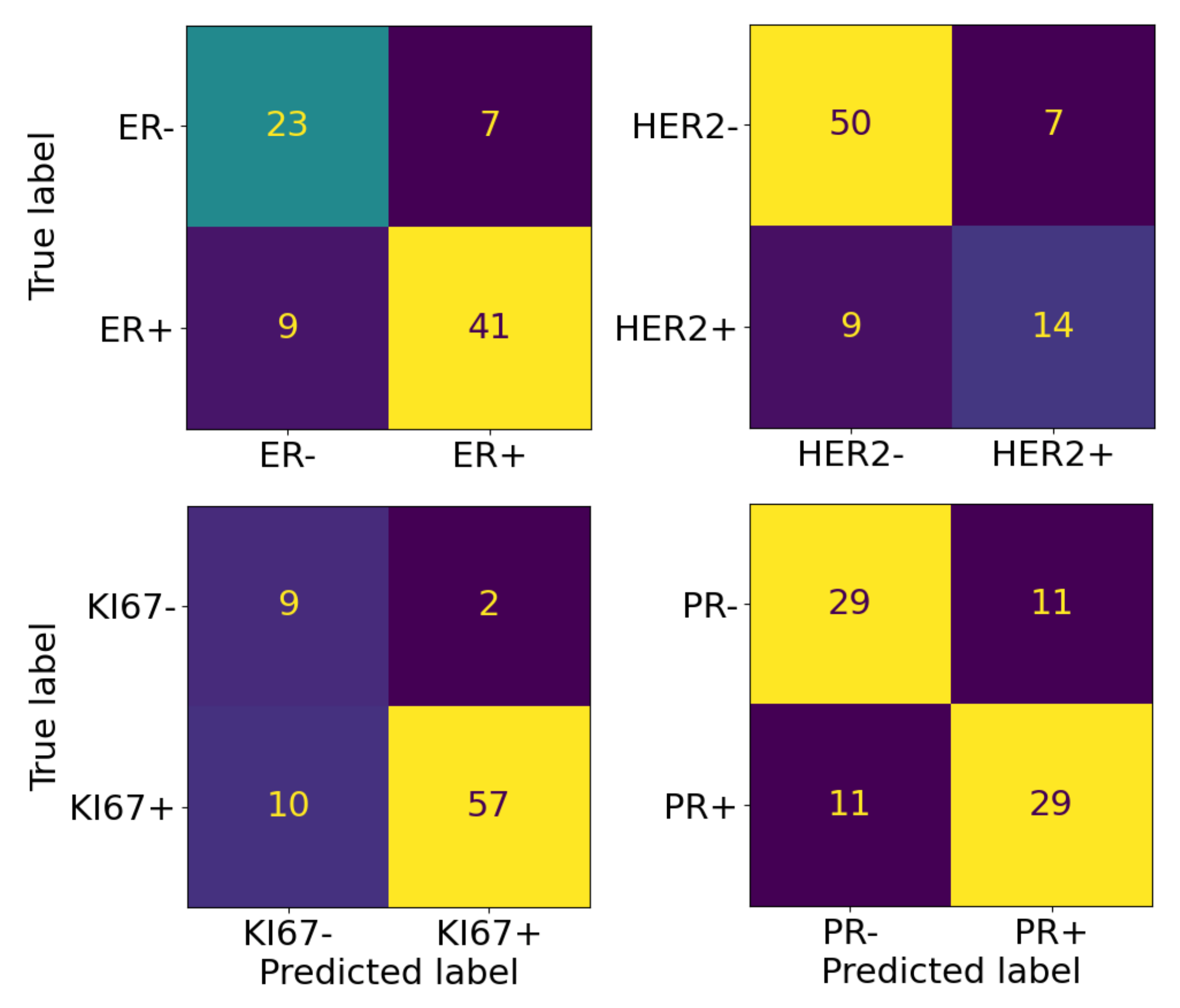
At the end of the two-step learning phase, the list of the most relevant features was obtained. Since the dataset size did not allow for a separate test set, and an external dataset with the same characteristics (e.g., same image type and modalities, same annotation markers) was missing, an LOOCV approach was applied to the original dataset to build the predictors. Hence, to further validate the results and simultaneously determine the best classification algorithm, a final step was performed using all the classification algorithms. The final feature list and the chosen classification algorithm constituted the final predictor. The bottom section of Figure 3 depicts this last step.
To assess the generalization abilities of the models and, more generally, the validity of the proposed two-step approach, the predictors were tested on the DS T .Unfortunately, only the predictors for the ER and PR markers can be tested since the available information regarding HER2 was partial or totally missing as in the case of Ki67. In addition, only the T1 and T2 images were present, whereas the ADC and SUB were unavailable. We used the same approach described above to assign samples to the classes whenever the needed information was available and the positive/negative official label otherwise. We ended up with 91 patients for both the ER and PC markers, with the classes distributed as follows: ER−/ER+ = ( 15.4 % / 84.6 % ) and PR−/PR+ = ( 20.9 % / 79.1 % ).
Therefore, only the ER and PR detection tests have been performed using the feature subset selected in the last step of the pipeline.

3. Results

3.1. Experiments and Settings

The proposed pipeline has been applied separately to the four molecular markers. Data from the DS M comply with the common practice in markers annotation, with ER, Ki67, and PR expressed in percentages (of involved cells), whereas the HER2 had discrete values followed, in this case, by one or more plus signs. To train the classification models, the markers’ expression values were binarized according to the following criteria: the ER and PR markers were considered negative if their value was lower than 10% and positive otherwise; the Ki67 marker was considered negative if it had a value lower than 14% and positive otherwise; and HER2 was considered negative if its value was 0 or 1 and positive otherwise [44]. The distribution of data classes obtained following those criteria is reported in Table 3. Except for the PR marker, the class distribution is strongly unbalanced. In the two-step feature classification process, the threshold t 1 , which should provide a coarse-grained feature subset, was set to t 1 = [ 5 , 10 , 15 , . . . , 50 ] , whereas the t 2 threshold was used to extract a fine-grained feature subset and was set to t 2 = [ 1 , . . . , 10 ] . These values were selected for: (i) having a comparable number of input samples and features in the classification steps and (ii) trying to extract a smaller, meaningful representative subset able to generalize across datasets. Due to the reduced number of input samples, a 10-fold cross-validation approach was used in the first two steps of the feature selection pipeline. Generally, when working on classification models in which the dataset is unbalanced, the F1-score, which combines precision and recall into a single metric, is a suitable measure. Thus, the F1-score was used to select the best training models. In the next subsections, the results of the first and second steps of the feature selection are reported separately. Moreover, different model settings were taken into account:
  • Radiomics from a single MRI sequence;
  • Radiomics from all MRI sequences;
  • Radiomics from a ingle MRI sequence + clinical information (i.e., patient’s age);
  • Radiomics from all MRI sequences + clinical information (i.e., patient’s age).
Regarding implementation details, both classifiers and feature selection algorithms have been implemented in Python 3.7, using the Scikit-learn framework [45] and scikit-feature package [46], respectively. As for the over-sampling algorithm SMOTE, we adopted the implementation provided by the Imbalanced-learn library [47].

3.2. Results of the First Feature Selection Step

All the experiments performed for the first step of the feature selection are available in the Supplementary Materials (Tables S1–S4). However, to give the reader an idea of the available information, some results are reported in Table 4. For each of the different input combinations, the best F1-score is shown. Features from different image modalities were taken all together or used separately. Considering the ER marker, the T2 modality emerged as the one performing better when using only radiomics features and also with a combination of radiomics and clinical data. When all the image modalities were used together, the performances decreased. Considering the HER2 marker, ADC was the modality giving the best results, whereas for Ki67, the best performances were obtained using all the image modalities and only the radiomics features. Finally, for the PR marker, the PC modality gave the best results both with clinical data and without them.
Referring to the Supplementary Tables S1–S4, the classification results obtained with the complete set of features were generally much worse than the ones obtained after the feature selection. This result was expected since the number of features was much higher than the number of input data. Hence, feature selection was confirmed to be a mandatory step when performing classification in these conditions.
The Supplementary Materials show the results obtained for all the possible combinations of features, namely those using all the radiomics modalities (thus totaling more than four thousand features for each patient), using both the radiomics and the clinical information, and using single radiomics modalities (about one thousand features for each patient). The two best results were considered for each feature combination, and the feature threshold and selection algorithm used for each of them was reported. On the feature subsets obtained from the two best results, the second pipeline step was then applied. In all the cases, the only clinical feature available (that is, the patient’s age) did not emerge as an important one. Hence, only the radiomics features were used. There is no preferred feature selection algorithm over the four biomarkers and the different feature combinations. The Fisher Score method was one of the most used, thus suggesting that it could be a good starting choice if one needs to perform a single feature selection step. When the imaging modalities were used together, the ReliefF method generally gave the best results due to its higher robustness to noise and redundancy. Nonetheless, both for the HER2 and Ki67 markers, on which ReliefF and Fisher Score gave the best results, the subsequent feature selection step performs better when using the second best (i.e., Gini Index for HER2 and Chi Squared method for Ki67, as reported in the following subsection). This might be due to the classification algorithm overfitting the selected features owing to the small dataset size. Regarding the radiomics modalities, the SUB one always gave poor results, whereas the T2 and PC were often preferred. The ADC alone never emerged, but it proved useful in combination with other modalities. In addition, for the t 1 threshold, there is no preferred value. The t 1 value giving the best results changes widely along the different modalities, features, and classification algorithms.

3.3. Results of the Second Feature Selection Step

The final classification results for all the markers obtained after the second feature selection step are shown in terms of F1-score in Table 5 and in terms of accuracy, precision, and recall in Table 6. In addition, in the second pipeline step, there was no clearly winning feature selection algorithm. LR-RFE and CFS gave the best results, with the MI approach performing generally worse. MLP is the classification algorithm more frequently used, although high results were also obtained with the DT and the KNN models (for the HER2 and PR markers, respectively). In the final step, the best-performing classification algorithm was chosen to obtain the final predictor. There was no preferred one, with MLP usually performing as well as the SVM, with the second being more prone to overfitting or learning a single class in the most unbalanced cases (as in Ki67).
The F1-scores for the LOOCV step were calculated considering the two labels in turn as the positive class. Indeed, for these markers, both the negative and positive states are important in defining the cancer’s molecular subtype. Especially in the case of the HER2 marker, whose class distribution was highly unbalanced, with 71% of samples belonging to the negative class, it was very important to understand how the predictor behaved. Being trained on a majority of negative samples, it performed better in detecting negative samples. However, it had good abilities also with a positive sample. When the classes were balanced, as in the PR case, there was no difference between the two values. Confusion matrices associated with performances of the predictors at the end of the two-step pipeline were reported in Figure 4.
The final feature number was obtained in the LOOCV step, and the list of the extracted features list is available in Table 7. For HER2, the best results were obtained with a combination of features coming from two different image modalities (i.e., ADC, T2). For the Ki67 and PR markers, the features all belong to the PC modality, whereas for the ER marker, they belong to the T2 one.
Concerning the validation performed on the DS T , a noteworthy F1-score of 0.88 was obtained for the ER marker. Since other works report their performances based on the Area Under the ROC curve (AUC), this measure was also computed for the ER marker, obtaining an AUC = 0.77. For the PR marker, results were less encouraging. The F1-score was 0.88, but only a single class (the positive one) was predicted on those data, thus resulting in an AUC = 0.63, as expected for this condition. Figure 5 shows the curves obtained for the two markers.

4. Discussion

This study aimed at comparing the performance of different radiomic models in the prediction of the four most widely used molecular markers (ER, HER2, Ki67, PR) in BC management, using a two-step feature selection radiomic approach to extract meaningful mpMRI feature subsets. Predictions were performed under different settings, i.e., with or without clinical features with radiomics and, for the latter, in all the mono- and multi-modality combinations of MRI sequences.
The results obtained in this study demonstrated that the proposed approach was an accurate method to pre-operatively predict the most relevant molecular markers, with the best resulting models composed of only radiomic features and reaching F1-scores up to 0.9. In particular, for HER2, the best results were obtained with an SVM model built with three T2 texture features and the minimum value of ADC from the LLH wavelet transformed ADC map. Other studies found that MRI-based features were associated with the HER2 status of patients with BC [48]. For the Ki67 and PR markers, the best results were obtained with an MLP model built with features all belonging to the PC modality, which currently represents the clinical standard for characterizing BC lesions [49]. These results are partially in accordance with some previous studies investigating the power of radiomics for Ki67 and PR status prediction [50,51,52], although they also found promising results arising from different sequences. Of note, shape flatness was the only shape feature that contributed both in the PR prediction model and in the best-performing model for the ER marker (RF), which was surprisingly built entirely on T2 features. Shape flatness characterizes the shape of the tumor, and in particular, a small flatness value indicates an irregular tumor shape. This feature has been shown to have power in the prognostic prediction of BC patients [53,54]. It is worth noting that, except for the prediction of HER2+ status, radiomics features are critical for model construction derived from a single MRI sequence.
From the methodological point of view, our two-step pipeline is novel, although it shares some similarities with approaches used in other works. In particular, in Xie et al. [55], a two-step pipeline was proposed to filter features, distinguishing between coarse-grained and fine-grained feature subsets with the classification target of simultaneously classifying the four immunohistochemically derived cancer subtypes. They reported a mean accuracy of 0.72 on a private dataset. Apart from being different in the imaging modalities and the learning targets used, they relied on a single statistical method for the first feature selection step, whereas we exploited several different algorithms to choose the most suitable one for the problem at hand. We suggested the importance of exploiting features coming from different imaging modalities, as also reported in Liu et al. [56], where they use conventional T2, DWI, and T1w DCE imaging to predict cancer subgroups and in particular to distinguish between HER2-positive/negative receptor status. They evaluated the performances on a private dataset and reported good results in the training phase (AUC = 0.78) and lower in the testing phase (AUC = 0.62), with better performances for the models exploiting multimodal features than monomodal ones. Notably, we found that for HER2, a multimodal feature set is needed to classify patients properly. This intuition was confirmed by the drop in F1-score to 0.57 when the ADC feature is removed. This result also underlines the critical importance of DWI for BC characterization, as also reported in previous studies [57].
Unfortunately, it was not possible to directly compare the results obtained with the proposed methodology with similar strategies on the same learning target, owing to the different, not publicly available dataset used. However some information could be extracted by looking at large-scale studies such as [58]: the authors exploited feature selection and machine learning (ML) approaches on a large private DCE-MRI dataset, obtaining an AUC = 0.65 for the ER status using training and test sets extracted from the same dataset. The result obtained in this study was higher, suggesting the good generalization abilities of the proposed predictor. In Li et al. [19], about forty radiomics features were extracted from the same TCGA-BRCA dataset we used, and the prediction ability of the features was assessed on the four clinical biomarkers through statistical analyses. Considering the ER biomarker prediction, they reached an AUC = 0.89. In Guo et al. [14] the authors used logistic regression to predict different outcomes, including the ER marker on which they obtained an AUC = 0.79. Again, a direct comparison was not possible since the predictors were built directly on the TCGA-BRCA data, while in this work, this dataset was only used as a test set (DS T ). However, it is essential to emphasize that the relevance of the obtained result lies in having the models trained on a dataset completely different from the one used to test them. Concerning the PR marker, the results from the already cited works reported AUCs of 0.62, 0.69, and 0.69, respectively. In this study, the predictor was not able to distinguish among the PR− /PR+ classes and assigned all the patients to the PR+ class. This was somehow expected given the differences between the used datasets and the small size of the training data and deserves to be further explored with the usage of additional data for the training phase. Referring to the Supplementary Materials, Table S5 reports a comparison of the experimental design adopted by the aforementioned works.
Despite the interesting results obtained, this study suffers from some limitations. First, the sample size for the analysis was small and, except for the PR+/PR− classification task, unbalanced. A larger and more balanced study group is needed to perform a better radiomic analysis and build more robust prediction models. Although the model’s performance was corrected by using 10-fold CV in the main classification step and LOOCV for the building of prediction models, such imbalance might have influenced the development of the ML model and the results [59]. Second, the study was retrospective and needed to be validated with other comprehensive external cohorts to determine the value of the developed model in clinical practice and improve the confidence of performance. Furthermore, prospective and multicentric studies need to be performed to define a potential standardization of the proposed approach. Moreover, the lack of standardization in radiomic investigations, in terms of image acquisition, processes, segmentation methods, and radiomics analysis tools, could lead to discrepancies in radiomic feature measurements that are not due to underlying biological variations.
Reproducibility of radiomic features is of crucial importance to clinical applications in the field of BC [60]. Of note, to extract radiomic features, we used the PyRadiomics software [61] which: (i) is compliant with the Image Biomarker Standardization Initiative (IBSI) guidelines that promoted the standardization of radiomic analysis [62], (ii) allows for a reproducible extraction of radiomic features due to the parameter files that could be shared and re-used, and (iii) can also be used starting from DICOM input images with the file name pointing to a DICOM Segmentation Image object, thus automatically obtaining radiomic features without any intermediate steps. This choice allows for a reproducible feature extraction under real clinical conditions that usually involve DICOM objects [27]. In addition, according to Lambin et al. [63], a detailed report of all the steps of the radiomic workflow performed in the study was carried out to improve both clinical translation in this emerging field and the reproducibility of study outcomes. Another limitation affecting this study concerned the use of manual segmentation for the VOIs’ delineation, which is time- and labor-consuming and prone to user variability. More accurate and automatic tumor segmentation tools are needed to improve the quality of the radiomic analysis in future works. On a positive note, in this study, 3D ROIs were used for lesion segmentation. The aim was to decrease inter-reader variability by eliminating the requirement to choose a single-slice corresponding to a portion of a lesion. Hence, a more thorough description of the lesion is obtained by an increase in the number of points considered for feature computation, which improved the accuracy of characterization of heterogeneous lesions and lowered the sampling errors [64].

5. Conclusions

The MRI-based radiomic approach developed in this work, built on a comprehensive BC dataset including MRI sequences and molecular outcomes, can efficiently characterize BC heterogeneity according to the most examined biomarkers (ER, PR, HER2, and Ki67). This methodology might be of great support for BC management for the following reasons: (i) it has the advantage of being developed on an appropriate two-step feature selection and classification technique; (ii) it implements an effective comparison of different models and feature selection approaches); (iii) it is externally validated whenever possible; and (iv) it addresses the well-known issues arising from the lack of available BC datasets by exploiting a comprehensive dataset of molecular markers and MRI modalities. Moreover, the developed two-step pipeline is general enough to be used on similar classification problems on different cancer types. Our results also highlighted the potential and strength of using only mpMRI data for high-quality BC radiomics analysis. Further prospective and multicentric studies need to be performed to define a potential standardization of our approach. In the future, larger BC cohorts will be investigated to validate our results more extensively.

Supplementary Materials

The following are available online at https://0-www-mdpi-com.brum.beds.ac.uk/article/10.3390/s23031552/s1, Tables S1–S4: Results of the first and second feature selection steps and of the final classification for the tasks ER+/ER−, HER2+/HER2−,KI67+/KI67−, PR+/PR2−; Table S5: Retrospective studies on predicting BC molecular subtypes.

Author Contributions

Conceptualization, M.A., G.D.P., V.R. and M.S. (Marco Salvatore); methodology, N.B., V.B. and M.S. (Mara Sangiovanni); software, M.L.R., G.E., C.A. and M.S. (Mara Sangiovanni); validation, N.B., V.B. and M.S. (Mara Sangiovanni); formal analysis, M.A., G.D.P., V.R., M.S. (Marco Salvatore) and M.S. (Mara Sangiovanni); data curation, V.B., G.E., C.C. and C.A.; supervision, M.A., G.D.P., V.R. and M.S. (Marco Salvatore). Writing—original draft preparation, N.B., V.B., G.E. and M.S. (Mara Sangiovanni). All authors have read and agreed to the published version of the manuscript.

Funding

This work was partially supported by the MIUR-PRIN2017 (grant 201744BN5T) project “Innovative methods of molecular imaging for oncological and neurodegenerative diseases-MOLIM ONCO BRAIN LAB”, PON Research and Innovation 2014–2020, Action II.2-Technological and partially supported by a “Ricerca Corrente” grant from the Italian Ministry of Health (IRCCS SYNLAB SDN).

Institutional Review Board Statement

This study was conducted in accordance with the Declaration of Helsinki, and the study protocol was approved by the ethics committee of the Istituto Nazionale Tumori “Fondazione G. Pascale” (protocol number 12/19 OSS SDN).

Informed Consent Statement

Informed consent was obtained from all subjects involved in the study.

Data Availability Statement

The DS M used in this paper come from the M O B L O B collection of BCU Imaging Biobank, available under request.

Acknowledgments

Some of the results here shown are based on the data provided by the TCGA Research Network: The Cancer Genome Atlas Program, https://www.cancer.gov/tcga, accessed on 1 September 2021.

Conflicts of Interest

The authors declare that they have no conflict of interest.

Abbreviations

The following abbreviations are used in this manuscript:
ADCApparent Diffusion Coefficient
AUCArea Under Receiver Operator Characteristic (ROC) Curve
BCBreast Cancer
CFSCorrelation-based Feature Selection
CNNConvolutional Neural Network
DCEDynamic Contrast-Enhanced
DICOMDigital Imaging and COmmunications in Medicine
DWIDiffusion Weighted Imaging
DTDecision Tree
EREstrogen Receptor
FSAFeature Selection Algorithm
GLCMGray-Level Co-occurrence Matrix
GLDMGray-Level Dependence Matrix
GLRLMGray-Level Run-Length Matrix
GLSZMGray-Level Size Zone Matrix
HER2Human Epidermal growth factor Receptor
IBSIImage Biomarker Standardization Initiative
KNNK-Nearest Neighbors
LALearning Algorithm
LASSOLeast Absolute Shrinkage and Selection Operator
LOOCVLeave-One-Out Cross-Validation
LRLASSO Regression
MIMutual Information
MLMachine Learning
MLPMulti Layer Perceptron
mpMRImultiparametric MRI
MRIMagnetic Resonance Imaging
NBNaive Bayes
NIfTINeuroimaging Informatics Technology Initiative
NGTDMNeighbouring Gray-Tone Difference Matrix
PCPost Contrast
PRProgesterone Receptor
RFRandom Forest
RFERecursive Features Elimination
ROCReceiver Operator Characteristic
ROIRegion Of Interest
SUBSubtracted
SVMSupport Vector Machine
SMOTESynthetic Minority Oversampling TEchnique
T2T2-weighted
TCIAThe Cancer Imaging Archive
TCGA-BRCAThe Cancer Genome Atlas BReast Invasive CArcinoma

References

  1. Sung, H.; Ferlay, J.; Siegel, R.L.; Laversanne, M.; Soerjomataram, I.; Jemal, A.; Bray, F. Global Cancer Statistics 2020: GLOBOCAN Estimates of Incidence and Mortality Worldwide for 36 Cancers in 185 Countries. CA Cancer J. Clin. 2021, 71, 209–249. [Google Scholar] [CrossRef] [PubMed]
  2. Wang, L. Early diagnosis of breast cancer. Sensors 2017, 17, 1572. [Google Scholar] [CrossRef] [Green Version]
  3. Tirada, N.; Aujero, M.; Khorjekar, G.; Richards, S.; Chopra, J.; Dromi, S.; Ioffe, O. Breast cancer tissue markers, genomic profiling, and other prognostic factors: A primer for radiologists. Radiographics 2018, 38, 1902–1920. [Google Scholar] [CrossRef] [Green Version]
  4. Woeckel, A.; Albert, U.S.; Janni, W.; Scharl, A.; Kreienberg, R.; Stueber, T. The screening, diagnosis, treatment, and follow-up of breast cancer. Dtsch. Ärzteblatt Int. 2018, 115, 316. [Google Scholar]
  5. Fisher, R.; Pusztai, L.; Swanton, C. Cancer heterogeneity: Implications for targeted therapeutics. Br. J. Cancer 2013, 108, 479–485. [Google Scholar] [CrossRef] [Green Version]
  6. Van’t Veer, L.J.; Dai, H.; Van De Vijver, M.J.; He, Y.D.; Hart, A.A.; Mao, M.; Peterse, H.L.; Van Der Kooy, K.; Marton, M.J.; Witteveen, A.T.; et al. Gene expression profiling predicts clinical outcome of breast cancer. Nature 2002, 415, 530–536. [Google Scholar] [CrossRef] [PubMed] [Green Version]
  7. Aiello, M. Is Radiomics Growing towards Clinical Practice? J. Pers. Med. 2022, 12, 1373. [Google Scholar] [CrossRef] [PubMed]
  8. Lambin, P.; Rios-Velazquez, E.; Leijenaar, R.; Carvalho, S.; Van Stiphout, R.G.; Granton, P.; Zegers, C.M.; Gillies, R.; Boellard, R.; Dekker, A.; et al. Radiomics: Extracting more information from medical images using advanced feature analysis. Eur. J. Cancer 2012, 48, 441–446. [Google Scholar] [CrossRef] [Green Version]
  9. Incoronato, M.; Aiello, M.; Infante, T.; Cavaliere, C.; Grimaldi, A.M.; Mirabelli, P.; Monti, S.; Salvatore, M. Radiogenomic analysis of oncological data: A technical survey. Int. J. Mol. Sci. 2017, 18, 805. [Google Scholar] [CrossRef] [Green Version]
  10. Monti, S.; Aiello, M.; Incoronato, M.; Grimaldi, A.M.; Moscarino, M.; Mirabelli, P.; Ferbo, U.; Cavaliere, C.; Salvatore, M. DCE-MRI pharmacokinetic-based phenotyping of invasive ductal carcinoma: A radiomic study for prediction of histological outcomes. Contrast Media Mol. Imaging 2018, 2018, 5076269. [Google Scholar] [CrossRef]
  11. Hylton, N. Dynamic contrast-enhanced magnetic resonance imaging as an imaging biomarker. J. Clin. Oncol. 2006, 24, 3293–3298. [Google Scholar] [CrossRef]
  12. Romeo, V.; Cavaliere, C.; Imbriaco, M.; Verde, F.; Petretta, M.; Franzese, M.; Stanzione, A.; Cuocolo, R.; Aiello, M.; Basso, L.; et al. Tumor segmentation analysis at different post-contrast time points: A possible source of variability of quantitative DCE-MRI parameters in locally advanced breast cancer. Eur. J. Radiol. 2020, 126, 108907. [Google Scholar] [CrossRef] [PubMed]
  13. Urruticoechea, A.; Smith, I.E.; Dowsett, M. Proliferation marker Ki-67 in early breast cancer. J. Clin. Oncol. 2005, 23, 7212–7220. [Google Scholar] [CrossRef] [PubMed]
  14. Guo, W.; Li, H.; Zhu, Y.; Lan, L.; Yang, S.; Drukker, K.; Morris, E.A.; Burnside, E.S.; Whitman, G.J.; Giger, M.L.; et al. Prediction of clinical phenotypes in invasive breast carcinomas from the integration of radiomics and genomics data. J. Med. Imaging 2015, 2, 041007. [Google Scholar] [CrossRef] [PubMed] [Green Version]
  15. Grimm, L.J.; Zhang, J.; Mazurowski, M.A. Computational approach to radiogenomics of breast cancer: Luminal A and luminal B molecular subtypes are associated with imaging features on routine breast MRI extracted using computer vision algorithms. J. Magn. Reson. Imaging 2015, 42, 902–907. [Google Scholar] [CrossRef]
  16. Mazurowski, M.A.; Zhang, J.; Grimm, L.J.; Yoon, S.C.; Silber, J.I. Radiogenomic analysis of breast cancer: Luminal B molecular subtype is associated with enhancement dynamics at MR imaging. Radiology 2014, 273, 365–372. [Google Scholar] [CrossRef]
  17. Sutton, E.J.; Oh, J.H.; Dashevsky, B.Z.; Veeraraghavan, H.; Apte, A.P.; Thakur, S.B.; Deasy, J.O.; Morris, E.A. Breast cancer subtype intertumor heterogeneity: MRI-based features predict results of a genomic assay. J. Magn. Reson. Imaging 2015, 42, 1398–1406. [Google Scholar] [CrossRef] [PubMed] [Green Version]
  18. Sutton, E.J.; Dashevsky, B.Z.; Oh, J.H.; Veeraraghavan, H.; Apte, A.P.; Thakur, S.B.; Morris, E.A.; Deasy, J.O. Breast cancer molecular subtype classifier that incorporates MRI features. J. Magn. Reson. Imaging 2016, 44, 122–129. [Google Scholar] [CrossRef] [PubMed] [Green Version]
  19. Li, H.; Zhu, Y.; Burnside, E.S.; Huang, E.; Drukker, K.; Hoadley, K.A.; Fan, C.; Conzen, S.D.; Zuley, M.; Net, J.M.; et al. Quantitative MRI radiomics in the prediction of molecular classifications of breast cancer subtypes in the TCGA/TCIA data set. NPJ Breast Cancer 2016, 2, 16012. [Google Scholar] [CrossRef] [PubMed] [Green Version]
  20. Sung, J.S.; Jochelson, M.S.; Brennan, S.; Joo, S.; Wen, Y.H.; Moskowitz, C.; Zheng, J.; Dershaw, D.D.; Morris, E.A. MR imaging features of triple-negative breast cancers. Breast J. 2013, 19, 643–649. [Google Scholar] [CrossRef]
  21. TCGA-BRCA. Available online: https://wiki.cancerimagingarchive.net/pages/viewpage.action?pageId=3539225 (accessed on 1 May 2021).
  22. Esposito, G.; Pagliari, G.; Randon, M.; Mirabelli, P.; Lavitrano, M.; Aiello, M.; Salvatore, M. BCU Imaging Biobank, an Innovative Digital Resource for Biomedical Research Collecting Imaging and Clinical Data From Human Healthy and Pathological Subjects. Open J. Bioresour. 2021, 8, 4. [Google Scholar] [CrossRef]
  23. Genomic Data Commons Data Portal. Available online: https://portal.gdc.cancer.gov/ (accessed on 1 May 2021).
  24. TCGA-Breast-Radiogenomics. Available online: https://wiki.cancerimagingarchive.net/pages/viewpage.action?pageId=19039112 (accessed on 1 May 2021).
  25. Haga, A.; Takahashi, W.; Aoki, S.; Nawa, K.; Yamashita, H.; Abe, O.; Nakagawa, K. Standardization of imaging features for radiomics analysis. J. Med. Investig. 2019, 66, 35–37. [Google Scholar] [CrossRef]
  26. Yu, J.S.; Chung, J.J.; Hong, S.W.; Chung, B.H.; Kim, J.H.; Kim, K.W. Prostate cancer: Added value of subtraction dynamic imaging in 3T magnetic resonance imaging with a phased-array body coil. Yonsei Med. J. 2008, 49, 765–774. [Google Scholar] [CrossRef] [PubMed] [Green Version]
  27. Fedorov, A.; Vangel, M.G.; Tempany, C.M.; Fennessy, F.M. Multiparametric magnetic resonance imaging of the prostate: Repeatability of volume and apparent diffusion coefficient quantification. Investig. Radiol. 2017, 52, 538. [Google Scholar] [CrossRef] [PubMed] [Green Version]
  28. Brancato, V.; Aiello, M.; Basso, L.; Monti, S.; Palumbo, L.; Di Costanzo, G.; Salvatore, M.; Ragozzino, A.; Cavaliere, C. Evaluation of a multiparametric MRI radiomic-based approach for stratification of equivocal PI-RADS 3 and upgraded PI-RADS 4 prostatic lesions. Sci. Rep. 2021, 11, 643. [Google Scholar] [CrossRef]
  29. Welcome to pyradiomics documentation! Available online: https://pyradiomics.readthedocs.io (accessed on 1 May 2021).
  30. Foster, K.R.; Koprowski, R.; Skufca, J.D. Machine learning, medical diagnosis, and biomedical engineering research-commentary. Biomed. Eng. Online 2014, 13, 94. [Google Scholar] [CrossRef] [PubMed] [Green Version]
  31. Kuhn, M.; Johnson, K. Applied Predictive Modeling; Springer: Berlin/Heidelberg, Germany, 2013; Volume 26. [Google Scholar]
  32. Guyon, I.; Gunn, S.; Nikravesh, M.; Zadeh, L.A. Feature Extraction: Foundations and Applications; Springer: Berlin/Heidelberg, Germany, 2008; Volume 207. [Google Scholar]
  33. Chawla, N.V.; Bowyer, K.W.; Hall, L.O.; Kegelmeyer, W.P. SMOTE: Synthetic minority over-sampling technique. J. Artif. Intell. Res. 2002, 16, 321–357. [Google Scholar] [CrossRef]
  34. Urso, A.; Fiannaca, A.; La Rosa, M.; Ravì, V.; Rizzo, R. Data Mining: Classification and Prediction. In Encyclopedia of Bioinformatics and Computational Biology; Elsevier: Amsterdam, The Netherlands, 2019; pp. 384–402. [Google Scholar] [CrossRef]
  35. Dasarathy, B.V. Nearest Neighbor (NN) Norms: NN Pattern Classification Techniques; IEEE Computer Society Tutorial; IEEE Computer Society: Washington, DC, USA, 1991. [Google Scholar]
  36. Langley, P.; Iba, W.; Thompson, K. An analysis of Bayesian classifiers. In Proceedings of the AAAI, San Jose, CA, USA, 12–16 July 1992; Citeseer: Princeton, NJ, USA, 1992; Volume 90, pp. 223–228. [Google Scholar]
  37. Vapnik, V. The Nature of Statistical Learning Theory; Springer Science & Business Media: Berlin, Germany, 2013. [Google Scholar]
  38. Magee, J.F. Decision Trees for Decision Making; Harvard Business Review: Brighton, MA, USA, 1964. [Google Scholar]
  39. Rumelhart, D.E.; Hinton, G.E.; Williams, R.J. Learning Internal Representations by Error Propagation; Technical report; California University San Diego La Jolla Inst for Cognitive Science: La Jolla, CA, USA, 1985. [Google Scholar]
  40. Ho, T.K. Random decision forests. In Proceedings of the 3rd International Conference on Document Analysis and Recognition, Montreal, QC, Canada, 14–16 August 1995; IEEE: Piscataway, NJ, USA, 1995; Volume 1, pp. 278–282. [Google Scholar]
  41. Ge, R.; Zhou, M.; Luo, Y.; Meng, Q.; Mai, G.; Ma, D.; Wang, G.; Zhou, F. McTwo: A two-step feature selection algorithm based on maximal information coefficient. BMC Bioinform. 2016, 17, 142. [Google Scholar] [CrossRef] [Green Version]
  42. Yang, R.; Zhang, C.; Zhang, L.; Gao, R. A two-step feature selection method to predict cancerlectins by multiview features and synthetic minority oversampling technique. BioMed Res. Int. 2018, 2018, 9364182. [Google Scholar] [CrossRef] [Green Version]
  43. Bolón-Canedo, V.; Alonso-Betanzos, A. Ensembles for feature selection: A review and future trends. Inf. Fusion 2019, 52, 1–12. [Google Scholar] [CrossRef]
  44. Santucci, D.; Faiella, E.; Cordelli, E.; Sicilia, R.; de Felice, C.; Zobel, B.B.; Iannello, G.; Soda, P. 3T MRI-Radiomic approach to predict for lymph node status in breast Cancer patients. Cancers 2021, 13, 2228. [Google Scholar] [CrossRef]
  45. Pedregosa, F.; Varoquaux, G.; Gramfort, A.; Michel, V.; Thirion, B.; Grisel, O.; Blondel, M.; Prettenhofer, P.; Weiss, R.; Dubourg, V.; et al. Scikit-learn: Machine Learning in Python. J. Mach. Learn. Res. 2011, 12, 2825–2830. [Google Scholar]
  46. Li, J.; Cheng, K.; Wang, S.; Morstatter, F.; Trevino, R.P.; Tang, J.; Liu, H. Feature selection: A data perspective. ACM Comput. Surv. (CSUR) 2018, 50, 94. [Google Scholar] [CrossRef] [Green Version]
  47. Lemaître, G.; Nogueira, F.; Aridas, C.K. Imbalanced-learn: A Python Toolbox to Tackle the Curse of Imbalanced Datasets in Machine Learning. J. Mach. Learn. Res. 2017, 18, 1–5. [Google Scholar]
  48. Huang, Y.; Wei, L.; Hu, Y.; Shao, N.; Lin, Y.; He, S.; Shi, H.; Zhang, X.; Lin, Y. Multi-parametric MRI-based radiomics models for predicting molecular subtype and androgen receptor expression in breast cancer. Front. Oncol. 2021, 11, 706733. [Google Scholar] [CrossRef] [PubMed]
  49. Mann, R.M.; Kuhl, C.K.; Kinkel, K.; Boetes, C. Breast MRI: Guidelines from the European society of breast imaging. Eur. Radiol. 2008, 18, 1307–1318. [Google Scholar] [CrossRef] [Green Version]
  50. Kayadibi, Y.; Kocak, B.; Ucar, N.; Akan, Y.N.; Akbas, P.; Bektas, S. Radioproteomics in breast cancer: Prediction of Ki-67 expression with MRI-based radiomic models. Acad. Radiol. 2022, 29, S116–S125. [Google Scholar] [CrossRef]
  51. Fan, M.; Yuan, W.; Zhao, W.; Xu, M.; Wang, S.; Gao, X.; Li, L. Joint prediction of breast cancer histological grade and Ki-67 expression level based on DCE-MRI and DWI radiomics. IEEE J. Biomed. Health Informatics 2019, 24, 1632–1642. [Google Scholar] [CrossRef] [Green Version]
  52. Zhong, S.; Wang, F.; Wang, Z.; Zhou, M.; Li, C.; Yin, J. Multiregional Radiomic Signatures Based on Functional Parametric Maps from DCE-MRI for Preoperative Identification of Estrogen Receptor and Progesterone Receptor Status in Breast Cancer. Diagnostics 2022, 12, 2558. [Google Scholar] [CrossRef]
  53. Fang, J.; Zhang, B.; Wang, S.; Jin, Y.; Wang, F.; Ding, Y.; Chen, Q.; Chen, L.; Li, Y.; Li, M.; et al. Association of MRI-derived radiomic biomarker with disease-free survival in patients with early-stage cervical cancer. Theranostics 2020, 10, 2284. [Google Scholar] [CrossRef]
  54. Park, H.; Lim, Y.; Ko, E.S.; Cho, H.h.; Lee, J.E.; Han, B.K.; Ko, E.Y.; Choi, J.S.; Park, K.W. Radiomics Signature on Magnetic Resonance Imaging: Association with Disease-Free Survival in Patients with Invasive Breast CancerRadiomics Signature on MRI for DFS in Invasive Breast Cancer. Clin. Cancer Res. 2018, 24, 4705–4714. [Google Scholar] [CrossRef] [PubMed] [Green Version]
  55. Xie, T.; Wang, Z.; Zhao, Q.; Bai, Q.; Zhou, X.; Gu, Y.; Peng, W.; Wang, H. Machine learning-based analysis of MR multiparametric radiomics for the subtype classification of breast cancer. Front. Oncol. 2019, 9, 505. [Google Scholar] [CrossRef] [PubMed]
  56. Liu, Z.; Li, Z.; Qu, J.; Zhang, R.; Zhou, X.; Li, L.; Sun, K.; Tang, Z.; Jiang, H.; Li, H.; et al. Radiomics of multiparametric MRI for pretreatment prediction of pathologic complete response to neoadjuvant chemotherapy in breast cancer: A multicenter study. Clin. Cancer Res. 2019, 25, 3538–3547. [Google Scholar] [CrossRef] [PubMed] [Green Version]
  57. Ni, M.; Zhou, X.; Liu, J.; Yu, H.; Gao, Y.; Zhang, X.; Li, Z. Prediction of the clinicopathological subtypes of breast cancer using a fisher discriminant analysis model based on radiomic features of diffusion-weighted MRI. BMC Cancer 2020, 20, 1073. [Google Scholar] [CrossRef]
  58. Saha, A.; Harowicz, M.R.; Grimm, L.J.; Kim, C.E.; Ghate, S.V.; Walsh, R.; Mazurowski, M.A. A machine learning approach to radiogenomics of breast cancer: A study of 922 subjects and 529 DCE-MRI features. Br. J. Cancer 2018, 119, 508–516. [Google Scholar] [CrossRef] [Green Version]
  59. Ubaldi, L.; Valenti, V.; Borgese, R.; Collura, G.; Fantacci, M.; Ferrera, G.; Iacoviello, G.; Abbate, B.; Laruina, F.; Tripoli, A.; et al. Strategies to develop radiomics and machine learning models for lung cancer stage and histology prediction using small data samples. Phys. Medica 2021, 90, 13–22. [Google Scholar] [CrossRef] [PubMed]
  60. Granzier, R.; Ibrahim, A.; Primakov, S.; Keek, S.; Halilaj, I.; Zwanenburg, A.; Engelen, S.; Lobbes, M.; Lambin, P.; Woodruff, H.; et al. Test–Retest Data for the Assessment of Breast MRI Radiomic Feature Repeatability. J. Magn. Reson. Imaging 2021, 56, 592–604. [Google Scholar] [CrossRef]
  61. Van Griethuysen, J.J.; Fedorov, A.; Parmar, C.; Hosny, A.; Aucoin, N.; Narayan, V.; Beets-Tan, R.G.; Fillion-Robin, J.C.; Pieper, S.; Aerts, H.J. Computational radiomics system to decode the radiographic phenotype. Cancer Res. 2017, 77, e104–e107. [Google Scholar] [CrossRef] [Green Version]
  62. Zwanenburg, A.; Vallières, M.; Abdalah, M.A.; Aerts, H.J.; Andrearczyk, V.; Apte, A.; Ashrafinia, S.; Bakas, S.; Beukinga, R.J.; Boellaard, R.; et al. The image biomarker standardization initiative: Standardized quantitative radiomics for high-throughput image-based phenotyping. Radiology 2020, 295, 328–338. [Google Scholar] [CrossRef] [Green Version]
  63. Lambin, P.; Leijenaar, R.T.; Deist, T.M.; Peerlings, J.; De Jong, E.E.; Van Timmeren, J.; Sanduleanu, S.; Larue, R.T.; Even, A.J.; Jochems, A.; et al. Radiomics: The bridge between medical imaging and personalized medicine. Nat. Rev. Clin. Oncol. 2017, 14, 749–762. [Google Scholar] [CrossRef] [Green Version]
  64. Parmar, C.; Rios Velazquez, E.; Leijenaar, R.; Jermoumi, M.; Carvalho, S.; Mak, R.H.; Mitra, S.; Shankar, B.U.; Kikinis, R.; Haibe-Kains, B.; et al. Robust radiomics feature quantification using semiautomatic volumetric segmentation. PLoS ONE 2014, 9, e102107. [Google Scholar] [CrossRef] [PubMed]
Figure 1. The steps of the adopted radiomics pipeline. They include MRI acquisition, tumor segmentation, feature extraction, feature selection, and model analysis.
Sensors 23 01552 g001
Figure 2. Example of primary BC lesion shown on a pretreatment breast MRI: (a) post-contrast T1 images, (b) DCE-MRI subtraction images with the highest mean signal intensity within the ROI, (c) ADC map, and (d) T2 images.
Sensors 23 01552 g002
Figure 3. A schematic view of the ensemble feature selection and classification steps underlying the building process of each predictive model. The first two steps involve 10-fold cross-validation on the training dataset. The last step is based on a leave-one-out cross-validation (LOOCV) approach to validate the combination of selected features and classification models. The best F-score values drive the choice of the classification algorithm at each step.
Sensors 23 01552 g003
Figure 4. Confusion matrix for the four markers at the end of the two-step pipeline.
Sensors 23 01552 g004
Figure 5. ROC curves and Area Under the Curve (AUC) for the ER and PR markers on the DS T validation dataset.
Sensors 23 01552 g005
Table 1. Technical details of acquired MRI sequences. TR = Repetition Time; TE = Time to Echo; FA = Flip Angle; ST = Slice Thickness; FOV = Field Of View; Aver. = average; Meas. = measurements.
SequenceTR (ms)TE (ms)FA ( )SlicesST
(mm)
Voxel SizeMatrixFOV
(mm)
Aver.Meas.Time
(min)
b-Value
(s/mm 2 )
TSE T254408180404.00.8 × 0.84483402-03:34-
DWI ax96007490254.01.8 × 1.81923403-04:4850/500/800
DCE5.471.752036 (slab1)3.61.7 × 1.719232016009:39-
HR Vibe T1-w fat sat8.694.3315176 (slab1)0.90.8 × 0.84483401-03:21-
Table 2. List of the feature selection methods used, with a brief classification of the type, approach, and returned results. LR-RFE: Lasso Regression with Recursive Feature Elimination; CFS: Correlation-based Feature Selection.
AlgorithmType
(Ranker/Subset)
Approach
(Filter/Wrapper)
Result
(Complete/Partial)
Chi SquaredRankerFilterComplete
Fisher ScoreRankerFilterComplete
Gini IndexRankerFilterComplete
Mutual InformationRankerFilterPartial
ReliefFRankerFilterComplete
LR-RFERankerWrapperPartial
CFSSubsetFilterPartial
Table 3. Thresholds used to define the DS M positive/negative classes, and the derived distribution of the samples among them.
Marker
Name
Total
Samples
Positive
Threshold
Sample Class # (%)
NegativePositive
ER80 10 % 30 ( 37.5 % ) 50 ( 62.5 % )
HER280≥2 57 ( 71 % ) 23 ( 29 % )
Ki6778 14 % 11 ( 14 % ) 67 ( 86 % )
PR80 10 % 40 ( 50 % ) 40 ( 50 % )
Table 4. Best results of the first feature selection step for all markers. For each combination of features (i.e., single radiomics, single radiomics with clinical information) and for each combination of modalities (i.e., all together (ALL) and single), the best mean F1-score obtained over the folds is shown. Bold font indicates the best results for each marker.
MarkerFeature TypeImage
Modality
Feature
Selection
Algorithm
Feature
Threshold
t1
F1-Score
± Variance
ERradiomics from
single modalities
T2fisher450.69 ± 0.02
radiomics from
single modalities/clinical
T2fisher25 0.68 ± 0.01
radiomics/clinicalALLchi50 0.65 ± 0.04
radiomicsALLchi25 0.59 ± 0.04
HER2radiomics from
single modalities
ADCreliefF300.7 ± 0.03
radiomics from
single modalities/clinical
ADCreliefF10 0.69 ± 0.03
radiomics/clinicalALLgini index10 0.68 ± 0.02
radiomicsALLreliefF30 0.62 ± 0.02
Ki67radiomics from
single modalities
PCchi10 0.77 ± 0.06
radiomics from
single modalities/clinical
PCgini index5 0.75 ± 0.05
radiomics/clinicalALLchi50 0.72 ± 0.03
radiomicsALLfisher200.79 ± 0.05
PRradiomics from
single modalities
PCfisher50.73 ± 0.03
radiomics from
single modalities/clinical
PCfisher50.73 ± 0.03
radiomics/clinicalALLreliefF15 0.67 ± 0.07
radiomicsALLreliefF15 0.67 ± 0.07
Table 5. Results for the four markers after the proposed two-step pipeline and the model validation and selection. The features and the learning algorithm obtained at the final LOOCV step are used to build the model predictors. Only the best result (in terms of F1-score) is shown here for each marker. Since the classes were unbalanced (except for the PR marker), the F1-score obtained considering both the label values as the positive class is reported. FSA: Feature Selection Algorithm; LA: Learning Algorithm.
Best Training Results
Marker
Name
1st Step Results2nd Step ResultsLOO Results
Feat.
Type
FSA t 1 F1-Score
±var
FSA t 2 F1-Score
±var
LAFeat.
#
F1-Score
pos/neg
ERT2fisher45 0.69 ± 0.02 lr rfe10 0.72 ± 0.01 svm110.85/0.81
HER2ALLgini10 0.68 ± 0.02 cfs5 0.75 ± 0.04 rf50.64/0.86
Ki67PCchi10 0.77 ± 0.06 cfs1 0.79 ± 0.05 mlp20.9/0.84
PRPCfisher5 0.73 ± 0.03 lr rfe3 0.74 ± 0.03 mlp30.73/0.73
Table 6. Results for the four markers in terms of other metrics: acc = accuracy; prec = precision; and rec = recall.
Best Training Results (Other Metrics)
Marker
Name
1st Step Result2nd Step ResultLOO Result
acc ± varprec ± varrec ± varacc ± varprec ± varrec ± varaccprecrec
ER0.73 ± 0.020.72 ± 0.020.7 ± 0.020.74 ± 0.010.74 ± 0.020.72 ± 0.010.810.870.82
HER20.73 ± 0.020.71 ± 0.020.71 ± 0.020.8 ± 0.020.75 ± 0.040.77 ± 0.040.80.670.61
KI670.89 ± 0.010.76 ± 0.060.8 ± 0.060.87 ± 0.020.78 ± 0.050.84 ± 0.050.850.970.85
PR0.74 ± 0.030.77 ± 0.030.74 ± 0.030.75 ± 0.020.79 ± 0.020.75 ± 0.020.730.730.73
Table 7. Selected features at the end of the two-step pipeline for the four biomarkers.
ER
original_shape_Flatness
T2_original_glcm_Idmn
T2_wavelet-LHH_glszm_ZoneEntropy
T2_wavelet-LHH_gldm_LargeDependenceLowGrayLevelEmphasis
T2_wavelet-LLH_glszm_SmallAreaLowGrayLevelEmphasis
T2_wavelet-LLH_gldm_SmallDependenceLowGrayLevelEmphasis
T2_wavelet-LLH_firstorder_Skewness
T2_log-sigma-4-0-mm-3D_glcm_Imc2
T2_log-sigma-4-0-mm-3D_firstorder_Skewness
T2_log-sigma-5-0-mm-3D_glszm_SmallAreaEmphasis
T2_log-sigma-5-0-mm-3D_firstorder_Skewness
HER2
T2_original_glrlm_RunVariance
T2_original_glrlm_LongRunEmphasis
T2_original_glszm_ZonePercentage
T2_original_gldm_DependenceNonUniformityNormalized
ADC_wavelet-LLH_firstorder_Minimum
Ki67
PC_wavelet-LHH_gldm_DependenceEntropy
PC_wavelet-HHL_gldm_SmallDependenceLowGrayLevelEmphasis
PR
original_shape_Flatness
PC_wavelet-LLH_glcm_Correlation
PC_wavelet-HHH_ngtdm_Busyness
Disclaimer/Publisher’s Note: The statements, opinions and data contained in all publications are solely those of the individual author(s) and contributor(s) and not of MDPI and/or the editor(s). MDPI and/or the editor(s) disclaim responsibility for any injury to people or property resulting from any ideas, methods, instructions or products referred to in the content.

