Space–Time Relationship between Short-Term Exposure to Fine and Coarse Particles and Mortality in a Nationwide Analysis of Korea: A Bayesian Hierarchical Spatio-Temporal Model

Abstract
:1. Introduction
2. Data and Methods
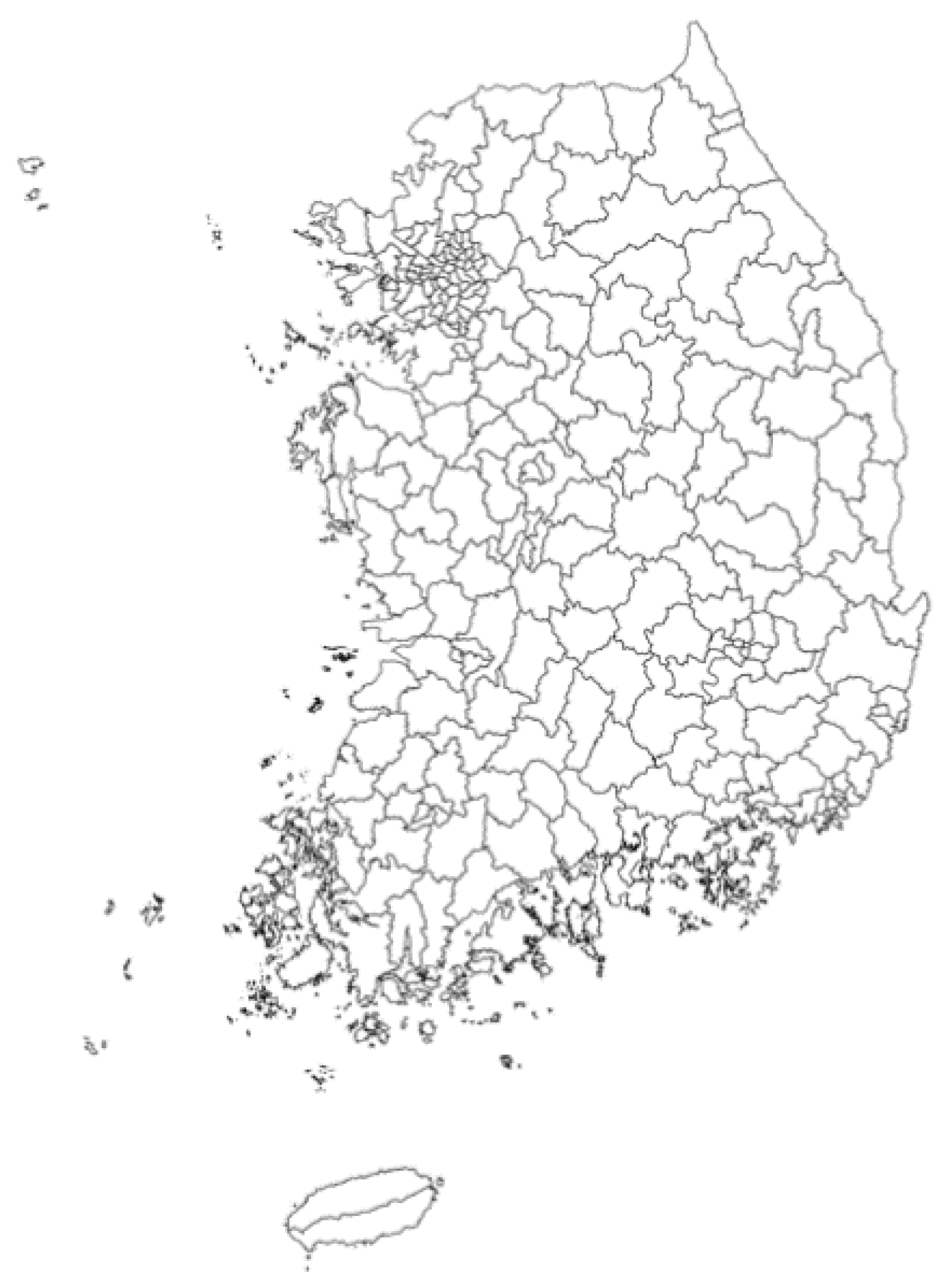
2.1. Study Domain
2.2. Data Description
2.3. Statistical Analysis
- Model 1:,
- Model 2: .
- Model 3:
3. Results
4. Discussion
5. Conclusions
Supplementary Materials
Author Contributions
Funding
Conflicts of Interest
References
- Samet, J.M.; Dominici, F.; Curriero, F.C.; Coursac, I.; Zeger, S.L. Fine particulate air pollution and mortality in 20 US cities, 1987–1994. N. Engl. J. Med. 2002, 343, 1742–1749. [Google Scholar] [CrossRef] [PubMed]
- Kwon, H.; Cho, S.; Chun, Y.; Lagarde, F.; Pershagen, G. Effects of the Asian dust events on daily mortality in Seoul, Korea. Environ. Res. 2002, 90, 1–5. [Google Scholar] [CrossRef] [PubMed]
- Ha, E.; Lee, J.; Kim, H.; Hong, Y.; Lee, B.; Park, H.; Christiani, D. Infant susceptibility of mortality to air pollution in Seoul, South Korea. Pediatrics 2003, 111, 284–290. [Google Scholar] [CrossRef] [PubMed]
- Kim, H.; Kim, Y.; Hong, Y. The lag-effect pattern in the relationship of particulate air pollution to daily mortality in Seoul, Korea. Int. J. Biometeorol. 2003, 48, 25–30. [Google Scholar] [CrossRef] [PubMed]
- Chen, R.; Kan, H.; Chen, B.; Huang, W.; Bai, Z.; Song, G.; Pan, G. Association of particulate air pollution with daily mortality: The China Air Pollution and Health Effects Study. Am. J. Epidemiol. 2012, 175, 1173–1181. [Google Scholar] [CrossRef] [PubMed]
- Pascal, M.; Corso, M.; Chanel, O.; Declercq, C.; Badaloni, C.; Cesaroni, G.; Medina, S. Assessing the public health impacts of urban air pollution in 25 European cities: Results of the Aphekom project. Sci. Total Environ. 2013, 449, 390–400. [Google Scholar] [CrossRef] [PubMed]
- Katsouyanni, K.; Touloumi, G.; Samoli, E.; Gryparis, A.; Le Tertre, A.; Monopolis, Y.; Rossi, G.; Zmirou, D.; Ballester, F.; Boumghar, A.; et al. Confounding and Effect Modification in the Short-Term Effects of Ambient Particles on Total Mortality: Results from 29 European Cities within the APHEA2 Project. Epidemiology 2001, 12, 521–531. [Google Scholar] [CrossRef] [PubMed] [Green Version]
- Dominici, F.; Peng, R.D.; Zeger, S.L.; White, R.H.; Samet, J.M. Particulate air pollution and mortality in the United States: Did the risks change from 1987 to 2000? Am. J. Epidemiol. 2007, 166, 880–888. [Google Scholar] [CrossRef]
- Woodruff, T.; Darrow, L.; Parker, J. Air pollution and postneonatal infant mortality in the United States, 1999–2002. Environ. Health Perspect. 2007, 116, 110–115. [Google Scholar] [CrossRef]
- Carlin, B.P.; Gelfand, A.E.; Banerjee, S. Hierarchical Modeling and Analysis for Spatial Data; Chapman and Hall CRC Press: Boca Raton, FL, USA, 2014. [Google Scholar]
- Cressie, N.; Wikle, C.K. Statistics for Spatio-Temporal Data; John Wiley & Sons: Hoboken, NJ, USA, 2015. [Google Scholar]
- Sahu, S.K.; Bakar, K.S. A comparison of Bayesian models for daily ozone concentration levels. Stat. Methodol. 2012, 9, 144–157. [Google Scholar] [CrossRef]
- Bakar, K.S.; Sahu, S.K. spTimer: Spatio-temporal bayesian modelling using R. J. Stat. Softw. 2015, 63, 1–32. [Google Scholar] [CrossRef]
- Del, S.S.; Ranalli, M.G.; Bakar, K.S.; Cappelletti, D.; Moroni, B.; Crocchianti, S.; Salvatori, R. Bayesian Spatiotemporal Modeling of Urban Air Pollution Dynamics. Top. Methodol. Appl. Stat. Inference 2016, 95–103. [Google Scholar] [CrossRef] [Green Version]
- Lawson, A.B.; Choi, J.; Cai, B.; Hossain, M.; Kirby, R.S.; Liu, J. Bayesian 2-stage space-time mixture modeling with spatial misalignment of the exposure in small area health data. J. Agric. Biol. Environ. Stat. 2012, 17, 417–441. [Google Scholar] [CrossRef] [PubMed]
- Liang, D.; Kumar, N. Time-space Kriging to address the spatiotemporal misalignment in the large datasets. Atmos. Environ. 2013, 72, 60–69. [Google Scholar] [CrossRef] [PubMed] [Green Version]
- James, S.H.; Brian, J.R. Adding spatially-correlated errors can mess up the fixed effect you love. Am. Stat. 2010, 64, 325–334. [Google Scholar] [CrossRef]
- Lee, H.; Kim, H.; Honda, Y.; Lim, Y.H.; Yi, S. Effect of Asian dust storms on daily mortality in seven metropolitan cities of Korea. Atmos. Environ. 2013, 79, 510–517. [Google Scholar] [CrossRef]
- Son, J.Y.; Lee, J.T.; Kim, H.; Yi, O.; Bell, M.L. Susceptibility to air pollution effects on mortality in Seoul, Korea: A case-crossover analysis of individual-level effect modifiers. J. Expo. Sci. Environ. Epidemiol. 2012, 22, 227. [Google Scholar] [CrossRef] [PubMed]
- Microdata Integrated Service Home Page. Available online: https://mdis.kostat.go.kr (accessed on 13 June 2019).
- Pun, K.; Seigneur, C. Using CMAQ to Interpolate among CASTNET Measurements; Atmospheric and Environmental Research Inc.: San Ramon, CA, USA, 2006. [Google Scholar]
- Choi, J.; Lawson, A.B. A Bayesian two-stage spatially dependent variable selection model for space–time health data. Stat. Methods Med. Res. 2018, 1–13. [Google Scholar] [CrossRef] [PubMed]
- Besag, J. Spatial interaction and the statistical analysis of lattice systems. J. R. Stat. Soc. Ser. B Stat. Methodol. 1974, 36, 192–236. [Google Scholar] [CrossRef]
- Knorr-Held, L. Bayesian modelling of inseparable space-time variation in disease risk. Stat. Med. 2000, 19, 2555–2567. [Google Scholar] [CrossRef]
- Bowman, D.D.; Liu, Y.; McMahan, C.S.; Nordone, S.K.; Yabsley, M.J.; Lund, R.B. Forecasting United States heartworm Dirofilaria immitis prevalence in dogs. Parasites Vectors 2016, 9, 540. [Google Scholar] [CrossRef] [PubMed]
- MRC Biostatistics Unit Home Page. Available online: https://www.mrc-bsu.cam.ac.uk/software/bugs/the-bugs-project-winbugs/ (accessed on 13 June 2019).
- Gelman, A.; Rubin, D.B. Inference from iterative simulation using multiple sequences. Stat. Sci. 1992, 7, 457–472. [Google Scholar] [CrossRef]
- The R Project for Statistical Computing Home Page. Available online: https://www.r-project.org (accessed on 13 June 2019).
- Park, A.; Hong, Y.; Kim, H. Effect of changes in season and temperature on mortality associated with air pollution in Seoul, Korea. J. Epidemiol. Community Health 2011, 65, 368–375. [Google Scholar] [CrossRef] [PubMed]
- Pope, C.A., III; Burnett, R.T.; Thun, M.J.; Calle, E.E.; Krewski, D.; Ito, K.; Thurston, G.D. Lung cancer, cardiopulmonary mortality, and long-term exposure to fine particulate air pollution. Jama 2002, 287, 1132–1141. [Google Scholar] [CrossRef] [PubMed]
- Jerrett, M.; Burnett, R.T.; Ma, R.; Pope, C.A., III; Krewski, D.; Newbold, K.B.; Thurston, G.; Shi, Y.; Finkelstein, N.; Calle, E.E.; et al. Spatial analysis of air pollution and mortality in Los Angeles. Epidemiology 2005, 16, 727–736. [Google Scholar] [CrossRef] [PubMed]
- World Health Organization. Quantification of Health Effects of Exposure to Air Pollution: Report on A WHO Working Group; WHO Regional Office for Europe: Copenhagen, Denmark, 2000. [Google Scholar]
- Kan, H.; London, S.J.; Chen, G.; Zhang, Y.; Song, G.; Zhao, N.; Jiang, L.; Chen, B. Season, sex, age, and education as modifiers of the effects of outdoor air pollution on daily mortality in Shanghai, China: The Public Health and Air Pollution in Asia (PAPA) Study. Environ. Health Perspect. 2008, 116, 1183–1188. [Google Scholar] [CrossRef] [PubMed]
- Burnett, R.T.; Brook, J.; Dann, T.; Delocla, C.; Philips, O.; Cakmak, S.; Vincent, R.; Goldberg, M.S.; Krewski, D. Association between particulate-and gas-phase components of urban air pollution and daily mortality in eight Canadian cities. Inhal. Toxicol. 2000, 12, 15–39. [Google Scholar] [CrossRef]


| Type | Variable | Unit | Mean | SD | Med | Q1 | Q3 | Min. | Max |
|---|---|---|---|---|---|---|---|---|---|
| Mortality | Total | person | 78.8 | 43.2 | 73 | 44 | 106 | 2 | 236 |
| Cardiovascular | person | 19.3 | 11.4 | 17 | 11 | 26 | 0 | 80 | |
| Respiratory | person | 7.7 | 4.8 | 7 | 4 | 10 | 0 | 35 | |
| Air pollutant | PM10 | µg/m3 | 37.7 | 12.1 | 36.8 | 28.8 | 46 | 3.7 | 83.2 |
| PM2.5 | µg/m3 | 29.4 | 10.5 | 28.3 | 21.5 | 36.7 | 1.6 | 69.6 | |
| Meteorological data | Temperature | °C | 13.2 | 9.6 | 14.1 | 5.2 | 21.7 | −7.9 | 29.7 |
| Humidity | % | 71 | 9 | 71.1 | 64.6 | 78.1 | 44.2 | 92.6 | |
| Wind speed | m/s | 2.9 | 0.9 | 2.7 | 2.3 | 3.3 | 1.3 | 8.2 | |
| Extra data | RDI | −0.1 | 8.4 | −1.3 | −6.8 | 6.6 | −22.5 | 16.5 | |
| Population | person | 202,196 | 154,313 | 170,220 | 60,151 | 308,111 | 18,036 | 669,068 |
| Model | MSPE | Deviance | pD | DIC |
|---|---|---|---|---|
| Model 1 | 184.22 | 72,690 | 11 | 72,701 |
| Model 2 | 77.09 | 63,597 | 548 | 64,145 |
| Model 3 | 79.25 | 63,098 | 10 | 63,108 |
| Air pollutant | Explanatory Variables | Total | Cardiovascular | Respiratory |
|---|---|---|---|---|
| Mean (95% CI) | Mean (95% CI) | Mean (95% CI) | ||
| PM10 | Air pollutant | 1.011 (1.008, 1.013) | 1.014 (1.009, 1.019) | 0.998 (0.991, 1.006) |
| Deprivation index | 1.001 (1.001, 1.002) | 1.003 (1.002, 1.004) | 1.016 (1.015, 1.017) | |
| PM2.5 | Air pollutant | 1.028 (1.026, 1.031) | 1.047 (1.042, 1.053) | 1.045 (1.036, 1.053) |
| Deprivation index | 1.001 (1.001, 1.001) | 1.003 (1.002, 1.004) | 1.016 (1.015, 1.017) |
© 2019 by the authors. Licensee MDPI, Basel, Switzerland. This article is an open access article distributed under the terms and conditions of the Creative Commons Attribution (CC BY) license (http://creativecommons.org/licenses/by/4.0/).
Share and Cite
Kang, D.; Jang, Y.; Choi, H.; Hwang, S.-s.; Koo, Y.; Choi, J. Space–Time Relationship between Short-Term Exposure to Fine and Coarse Particles and Mortality in a Nationwide Analysis of Korea: A Bayesian Hierarchical Spatio-Temporal Model. Int. J. Environ. Res. Public Health 2019, 16, 2111. https://0-doi-org.brum.beds.ac.uk/10.3390/ijerph16122111
Kang D, Jang Y, Choi H, Hwang S-s, Koo Y, Choi J. Space–Time Relationship between Short-Term Exposure to Fine and Coarse Particles and Mortality in a Nationwide Analysis of Korea: A Bayesian Hierarchical Spatio-Temporal Model. International Journal of Environmental Research and Public Health. 2019; 16(12):2111. https://0-doi-org.brum.beds.ac.uk/10.3390/ijerph16122111
Chicago/Turabian StyleKang, Dayun, Yujin Jang, Hyunho Choi, Seung-sik Hwang, Younseo Koo, and Jungsoon Choi. 2019. "Space–Time Relationship between Short-Term Exposure to Fine and Coarse Particles and Mortality in a Nationwide Analysis of Korea: A Bayesian Hierarchical Spatio-Temporal Model" International Journal of Environmental Research and Public Health 16, no. 12: 2111. https://0-doi-org.brum.beds.ac.uk/10.3390/ijerph16122111