What Are the Driving Forces of Urban CO2 Emissions in China? A Refined Scale Analysis between National and Urban Agglomeration Levels

Abstract
:1. Introduction
- (1)
- quantifying the driving forces of urban CO2 emissions at a finer spatial resolution (e.g., 1-km spatial resolution) using multiple-source data from 2000 to 2015;
- (2)
- evaluating the driving forces of urban CO2 emissions from multiple spatial levels;
- (3)
- comparing regional differences in the driving forces of urban CO2 emissions.
2. Data and Methods
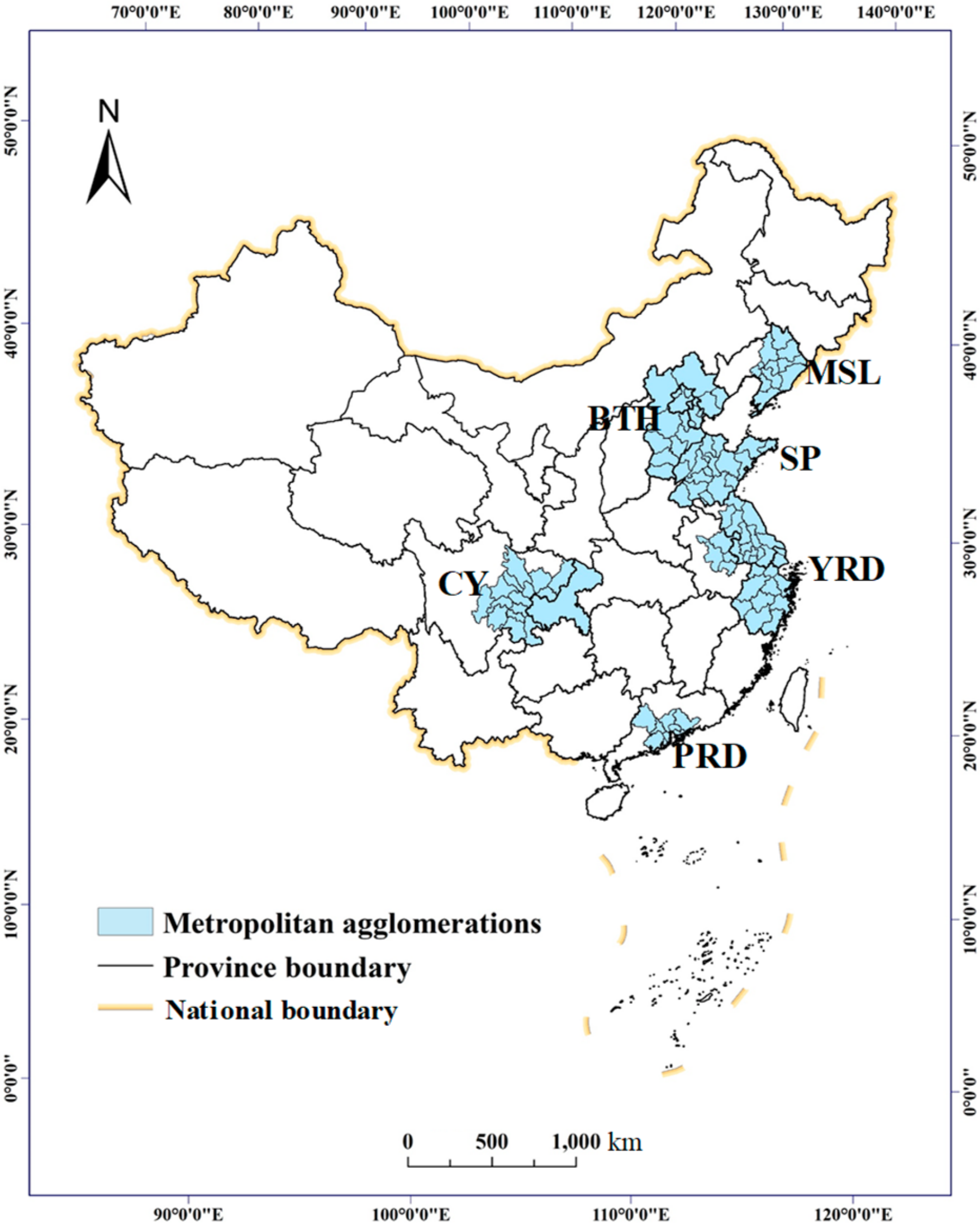
2.1. Study Areas
2.2. Urban CO2 Emissions
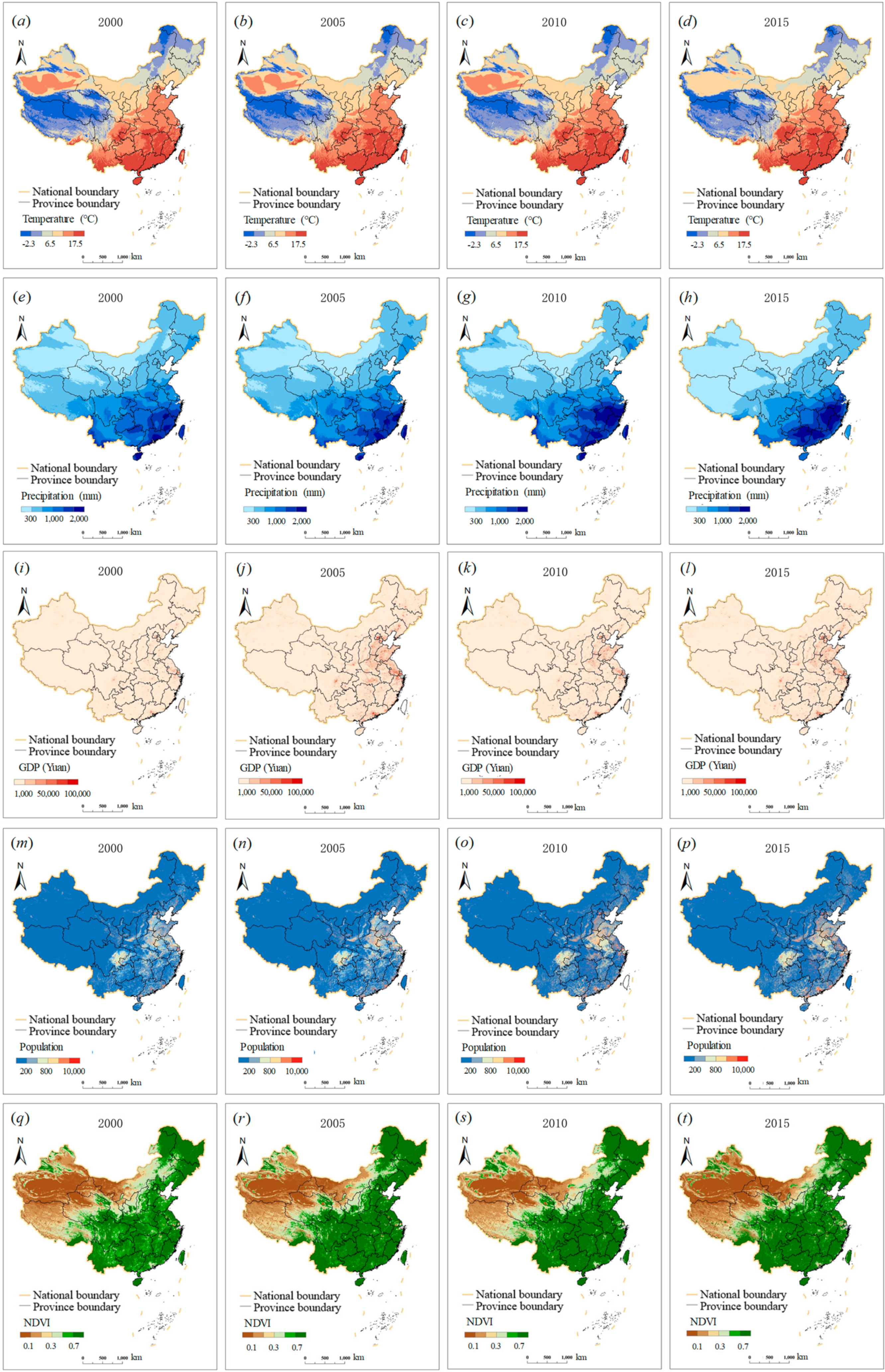
2.3. Potential Driving Forces
2.4. Probit Model
3. Results
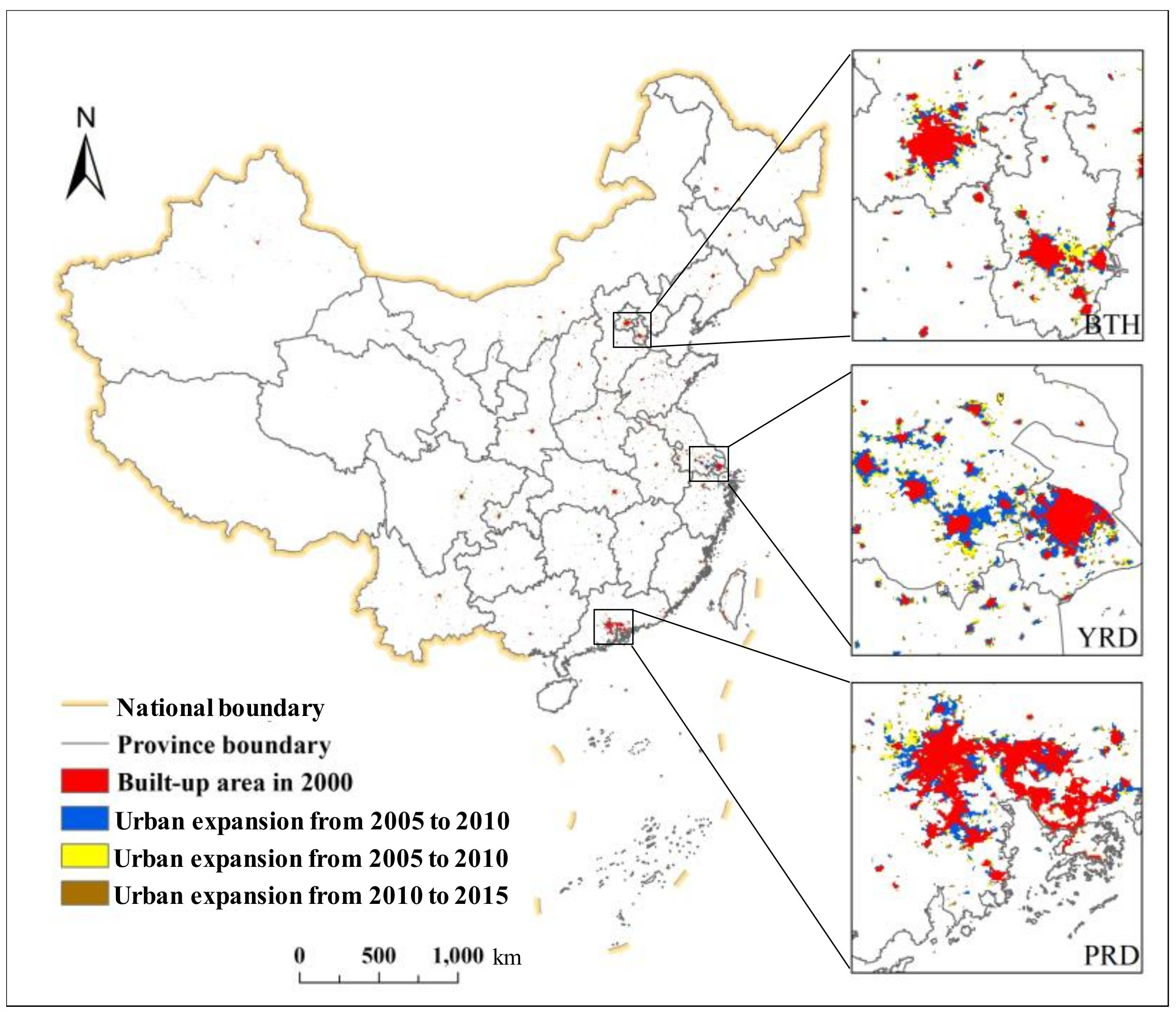
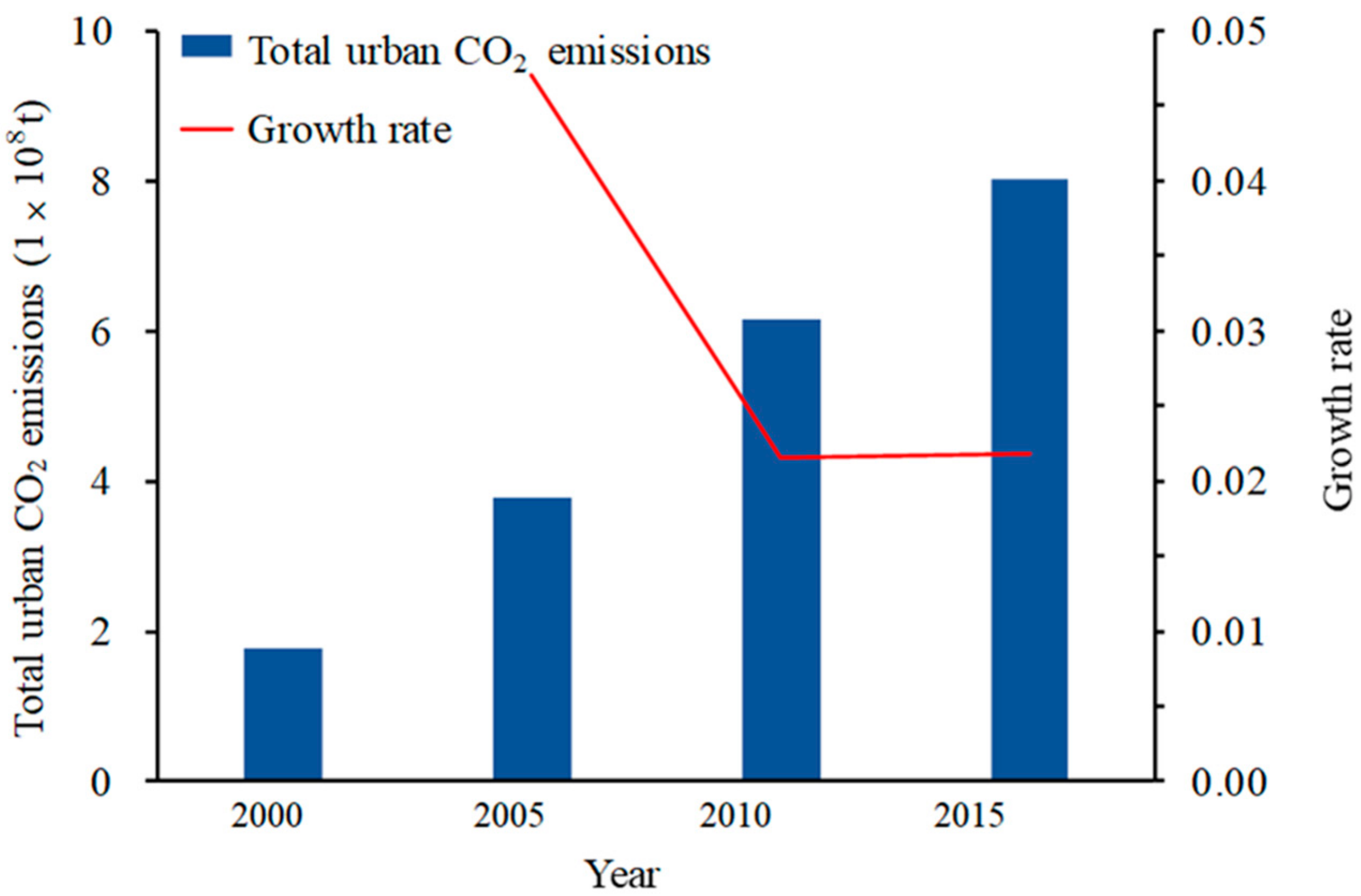
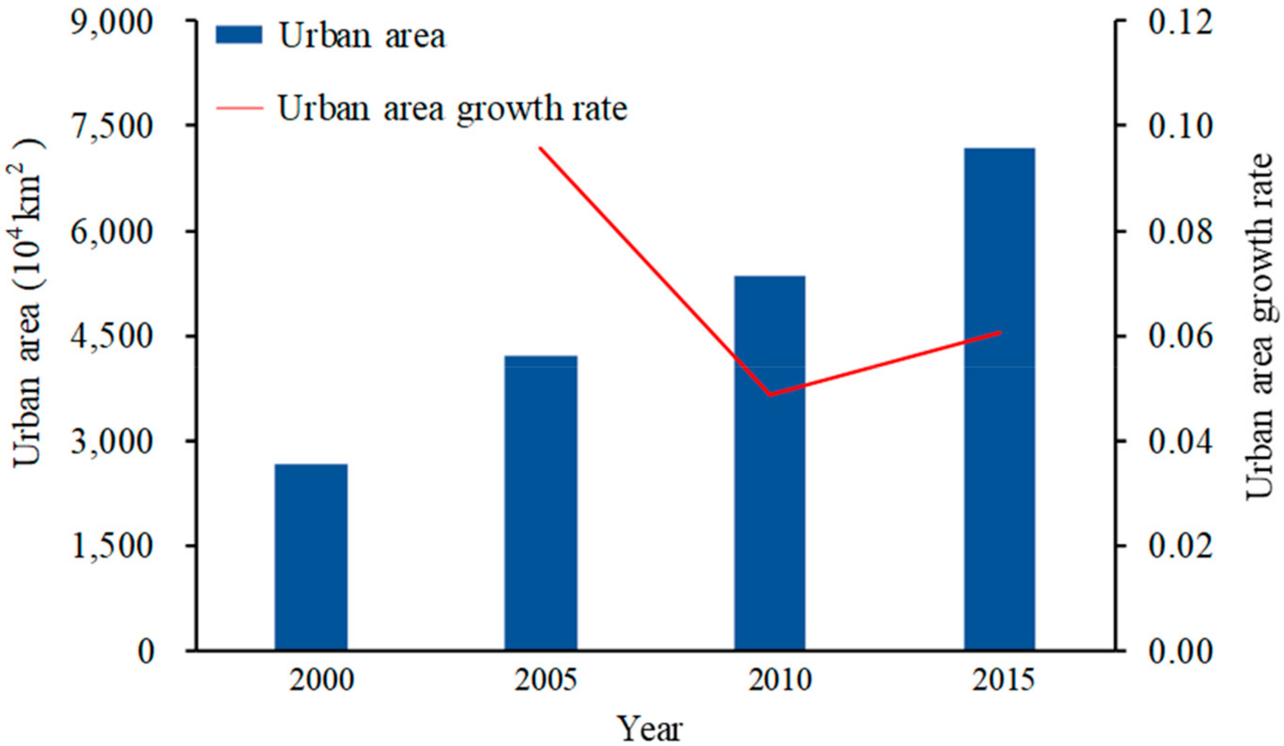
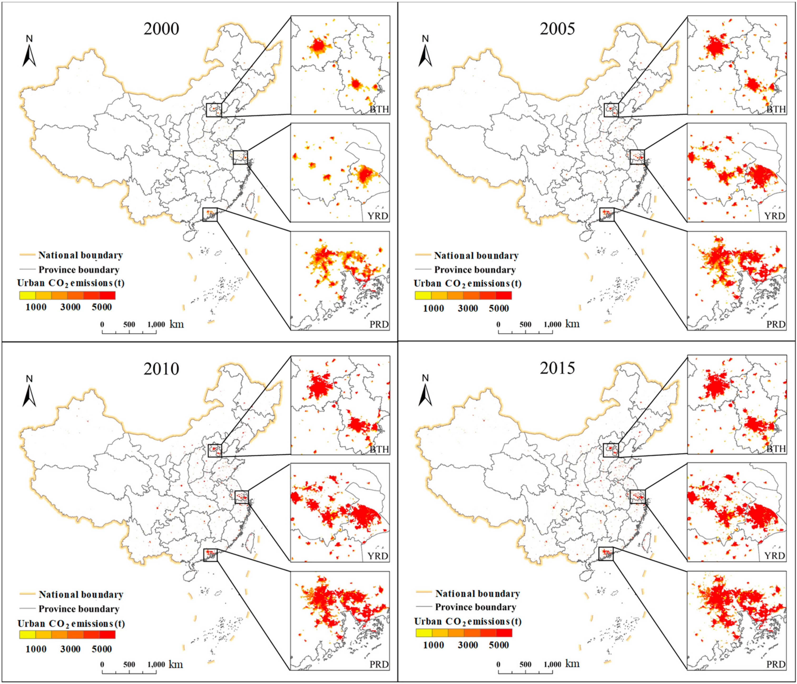
3.1. Spatiotemporal Variations of Urban CO2 Emissions
3.2. Results of the Driving Forces of Urban CO2 Emissions at the National Level
3.3. Results of the Driving Forces of Urban CO2 Emissions at the Urban Agglomeration Level
4. Discussion
4.1. Driving Forces of Urban CO2 Emissions at the National Level
4.2. Difference in the Driving Forces of Urban CO2 Emissions in the Six Urban Agglomerations
4.3. Difference in the Driving Forces of Urban CO2 Emissions at the Two Levels
4.4. Limitations and Future Directions
5. Conclusions and Policy Implications
Supplementary Materials
Author Contributions
Funding
Conflicts of Interest
References
- Davis, M.; Ahiduzzaman, M.; Kumar, A. How will Canada’s greenhouse gas emissions change by 2050? A disaggregated analysis of past and future greenhouse gas emissions using bottom-up energy modelling and Sankey diagrams. Appl. Energy 2018, 220, 754–786. [Google Scholar] [CrossRef]
- Zeng, S.; Jiang, C.; Ma, C.; Su, B. Investment efficiency of the new energy industry in China. Energy Econ. 2018, 70, 536–544. [Google Scholar] [CrossRef]
- Meinshausen, M.; Meinshausen, N.; Hare, W.; Raper, S.C.B.; Frieler, K.; Knutti, R.; Frame, D.J.; Allen, M.R. Greenhouse-gas emission targets for limiting global warming to 2 °C. Nature 2009, 458, 1158–1162. [Google Scholar] [CrossRef]
- Ou, J.; Liu, X.; Li, X.; Chen, Y. Quantifying the relationship between urban forms and carbon emissions using panel data analysis. Landsc. Ecol. 2013, 28, 1889–1907. [Google Scholar] [CrossRef]
- Seto, K.C.; Güneralp, B.; Hutyra, L.R. Global forecasts of urban expansion to 2030 and direct impacts on biodiversity and carbon pools. Proc. Natl. Acad. Sci. USA 2012, 109, 16083–16088. [Google Scholar] [CrossRef] [Green Version]
- Sun, M.; Wang, Y.; Lei, S. Uncovering energy use, carbon emissions and environmental burdens of pulp and paper industry: A systematic review and meta-analysis. Renew. Sustain. Energy Rev. 2018, 92, 823–833. [Google Scholar] [CrossRef]
- Clark, P.U.; Shakun, J.D.; Marcott, S.A.; Mix, A.C.; Eby, M.; Kulp, S.; Levermann, A.; Milne, G.A.; Pfister, P.L.; Santer, B.D.; et al. Consequences of twenty-first-century policy for multi-millennial climate and sea-level change. Nat. Clim. Chang. 2016, 6, 360–369. [Google Scholar] [CrossRef]
- Chen, Y.; Ebenstein, A.; Greenstone, M.; Li, H. Evidence on the impact of sustained exposure to air pollution on life expectancy from China’s Huai River policy. Proc. Natl. Acad. Sci. USA 2013, 110, 12936–12941. [Google Scholar] [CrossRef]
- Cai, B.; Zhang, L. Urban CO2 emissions in China: Spatial boundary and performance comparison. Energy Policy 2014, 66, 557–567. [Google Scholar] [CrossRef]
- Shi, K.; Chen, Y.; Li, L.; Huang, C. Spatiotemporal variations of urban CO2 emissions in China: A multiscale perspective. Appl. Energy 2018, 211, 218–229. [Google Scholar] [CrossRef]
- Cannistraro, M.; Ponterio, L.; Cao, J. Experimental study of air pollution in the urban centre of the city of Messina. Model. Meas. Control C 2018, 79, 133–139. [Google Scholar] [CrossRef]
- International Energy Agency. World Energy Outlook 2012; International Energy Agency: Paris, France, 2012. [Google Scholar]
- Cannistraro, G.; Cannistraro, M.; Cao, J.; Ponterio, L. New technique monitoring and transmission environmental data with mobile systems. Instrum. Mes. Metrol. 2018, 17, 549–562. [Google Scholar] [CrossRef]
- Shi, K.; Chen, Y.; Yu, B.; Xu, T.; Yang, C.; Li, L.; Huang, C.; Chen, Z.; Liu, R.; Wu, J. Detecting spatiotemporal dynamics of global electric power consumption using DMSP-OLS nighttime stable light data. Appl. Energy 2016, 184, 450–463. [Google Scholar] [CrossRef]
- Cannistraro, G.; Cannistraro, M.; Cannistraro, A.; Galvagno, A.; Engineer, F. Analysis of air pollution in the urban center of four cities Sicilian. Int. J. Heat Technol 2016, 34, S219–S225. [Google Scholar] [CrossRef]
- Xia, Y.; Wang, H.; Liu, W. The indirect carbon emission from household consumption in China between 1995–2009 and 2010–2030: A decomposition and prediction analysis. Comput. Ind. Eng. 2019, 128, 264–276. [Google Scholar] [CrossRef]
- Shi, K.; Yu, B.; Zhou, Y.; Chen, Y.; Yang, C.; Chen, Z.; Wu, J. Spatiotemporal variations of CO2 emissions and their impact factors in China: A comparative analysis between the provincial and prefectural levels. Appl. Energy 2019, 233–234, 170–181. [Google Scholar] [CrossRef]
- Gregg, J.S.; Andres, R.J.; Marland, G. China: Emissions pattern of the world leader in CO2 emissions from fossil fuel consumption and cement production. Geophys. Res. Lett. 2008, 35. [Google Scholar] [CrossRef]
- Bai, Y.; Deng, X.; Gibson, J.; Zhao, Z.; Xu, H. How does urbanization affect residential CO2 emissions? An analysis on urban agglomerations of China. J. Clean Prod. 2019, 209, 876–885. [Google Scholar] [CrossRef]
- Du, S.; He, C.; Huang, Q.; Shi, P. How did the urban land in floodplains distribute and expand in China from 1992–2015? Environ. Res. Lett. 2018, 13, 034018. [Google Scholar] [CrossRef]
- Wang, Y.; Li, X.; Kang, Y.; Chen, W.; Zhao, M.; Li, W. Analyzing the impact of urbanization quality on CO2 emissions: What can geographically weighted regression tell us? Renew. Sustain. Energy Rev. 2019, 104, 127–136. [Google Scholar] [CrossRef]
- Xu, Q.; Dong, Y.; Yang, R.; Zhang, H.; Wang, C.; Du, Z. Temporal and spatial differences in carbon emissions in the Pearl River Delta based on multi-resolution emission inventory modeling. J. Clean Prod. 2019, 214, 615–622. [Google Scholar] [CrossRef]
- Li, M.; Mi, Z.; Coffman, D.M.; Wei, Y.-M. Assessing the policy impacts on non-ferrous metals industry’s CO2 reduction: Evidence from China. J. Clean. Prod. 2018, 192, 252–261. [Google Scholar] [CrossRef]
- Han, J.; Meng, X.; Zhou, X.; Yi, B.; Liu, M.; Xiang, W.-N. A long-term analysis of urbanization process, landscape change, and carbon sources and sinks: A case study in China’s Yangtze River Delta region. J. Clean Prod. 2017, 141, 1040–1050. [Google Scholar] [CrossRef]
- Wang, S.; Li, G.; Fang, C. Urbanization, economic growth, energy consumption, and CO2 emissions: Empirical evidence from countries with different income levels. Renew. Sustain. Energy Rev. 2018, 81, 2144–2159. [Google Scholar] [CrossRef]
- Wang, M.; Yue, C.; Kai, Y.; Min, W.; Xiong, L.; Huang, Y. A local-scale low-carbon plan based on the STIRPAT model and the scenario method: The case of Minhang District, Shanghai, China. Energy Policy 2011, 39, 6981–6990. [Google Scholar] [CrossRef]
- Cai, B. CO2 emissions in four urban boundaries of China-Case study of Chongqing. China Environ. Sci. 2014, 34, 2439–2448. (In Chinese) [Google Scholar]
- Fang, C.; Wang, S.; Li, G. Changing urban forms and carbon dioxide emissions in China: A case study of 30 provincial capital cities. Appl. Energy 2015, 158, 519–531. [Google Scholar] [CrossRef]
- Zeng, S.; Xin, N.; Chao, L.; Chen, J. The response of the Beijing carbon emissions allowance price (BJC) to macroeconomic and energy price indices. Energy Policy 2017, 106, 111–121. [Google Scholar] [CrossRef]
- Wang, S.; Zhou, C.; Feng, K. Examining the socioeconomic determinants of CO2 emissions in China: A historical and prospective analysis. Resour. Conserv. Recycl. 2018, 130, 1–11. [Google Scholar]
- Wang, C.; Wu, K.; Zhang, X.; Wang, F.; Zhang, H.; Ye, Y.; Wu, Q.; Huang, G.; Wang, Y.; Wen, B. Features and drivers for energy-related carbon emissions in mega city: The case of Guangzhou, China based on an extended LMDI model. PLoS ONE 2019, 14, e0210430. [Google Scholar] [CrossRef]
- Wang, C.; Zhan, J.; Li, Z.; Zhang, F.; Zhang, Y. Structural decomposition analysis of carbon emissions from residential consumption in the Beijing-Tianjin-Hebei region, China. J. Clean Prod. 2019, 208, 1357–1364. [Google Scholar] [CrossRef]
- Wen, L.; Zhang, X. CO2 Emissions in China’s Yangtze River Economic Zone: A Dynamic Vector Autoregression Approach. Pol. J. Environ. Stud. 2019, 28, 923–933. [Google Scholar] [CrossRef]
- Wang, S.; Liu, X.; Zhou, C.; Hu, J.; Ou, J. Examining the impacts of socioeconomic factors, urban form, and transportation networks on CO2 emissions in China’s megacities. Appl. Energy 2017, 185, 189–200. [Google Scholar] [CrossRef]
- Miao, L. Examining the impact factors of urban residential energy consumption and CO2 emissions in China – Evidence from city-level data. Ecol. Indic. 2017, 73, 29–37. [Google Scholar] [CrossRef]
- Cao, X.; Wang, J.; Chen, J.; Shi, F. Spatialization of electricity consumption of China using saturation-corrected DMSP-OLS data. Int. J. Appl. Earth Obs. Geoinf. 2014, 28, 193–200. [Google Scholar] [CrossRef]
- Bereitschaft, B.; Debbage, K. Urban form, air pollution, and CO2 emissions in large U.S. metropolitan areas. Prof. Geogr. 2013, 65, 612–635. [Google Scholar] [CrossRef]
- Mccarty, J.; Kaza, N. Urban form and air quality in the United States. Landsc. Urban Plan. 2015, 139, 168–179. [Google Scholar] [CrossRef]
- Shi, K.; Chen, Y.; Yu, B.; Xu, T.; Chen, Z.; Liu, R.; Li, L.; Wu, J. Modeling spatiotemporal CO2 (carbon dioxide) emission dynamics in China from DMSP-OLS nighttime stable light data using panel data analysis. Appl. Energy 2016, 168, 523–533. [Google Scholar] [CrossRef]
- Wang, S.; Wang, J.; Fang, C.; Li, S. Estimating the impacts of urban form on CO2 emission efficiency in the Pearl River Delta, China. Cities 2019, 85, 117–129. [Google Scholar] [CrossRef]
- Li, F.; Zhou, T. Effects of urban form on air quality in China: An analysis based on the spatial autoregressive model. Cities 2019, 89, 130–140. [Google Scholar] [CrossRef]
- Zhao, J.; Ji, G.; Yue, Y.; Lai, Z.; Chen, Y.; Yang, D.; Yang, X.; Wang, Z. Spatio-temporal dynamics of urban residential CO2 emissions and their driving forces in China using the integrated two nighttime light datasets. Appl. Energy 2019, 235, 612–624. [Google Scholar] [CrossRef]
- Feng, Y.Y.; Chen, S.Q.; Zhang, L.X. System dynamics modeling for urban energy consumption and CO2 emissions: A case study of Beijing, China. Ecol. Model. 2013, 252, 44–52. [Google Scholar] [CrossRef]
- Ma, Q.; He, C.; Wu, J. Behind the rapid expansion of urban impervious surfaces in China: Major influencing factors revealed by a hierarchical multiscale analysis. Land Use Policy 2016, 59, 434–445. [Google Scholar] [CrossRef]
- Kolaczyk, E.D.; Huang, H. Multiscale statistical models for hierarchical spatial aggregation. Geogr. Anal. 2001, 33, 95–118. [Google Scholar] [CrossRef]
- Shi, K.; Chen, Y.; Yu, B.; Xu, T.; Li, L.; Huang, C.; Liu, R.; Chen, Z.; Wu, J. Urban expansion and agricultural land loss in China: A multiscale perspective. Sustainability 2016, 8, 790. [Google Scholar] [CrossRef]
- Shi, K.; Yang, Q.; Li, Y.; Sun, X. Mapping and evaluating cultivated land fallow in Southwest China using multisource data. Sci. Total Environ. 2019, 654, 987–999. [Google Scholar] [CrossRef]
- Su, Y.; Chen, X.; Li, Y.; Liao, J.; Ye, Y.; Zhang, H.; Huang, N.; Kuang, Y. China’s 19-year city-level carbon emissions of energy consumptions, driving forces and regionalized mitigation guidelines. Renew. Sustain. Energy Rev. 2014, 35, 231–243. [Google Scholar] [CrossRef]
- Shi, K.; Huang, C.; Yu, B.; Yin, B.; Huang, Y.; Wu, J. Evaluation of NPP-VIIRS night-time light composite data for extracting built-up urban areas. Remote Sens. Lett. 2014, 5, 358–366. [Google Scholar] [CrossRef]
- Ma, T.; Zhou, Y.; Zhou, C.; Haynie, S.; Pei, T.; Xu, T. Night-time light derived estimation of spatio-temporal characteristics of urbanization dynamics using DMSP/OLS satellite data. Remote Sens. Environ. 2015, 158, 453–464. [Google Scholar] [CrossRef]
- Liu, Z.; He, C.; Zhang, Q.; Huang, Q.; Yang, Y. Extracting the dynamics of urban expansion in China using DMSP-OLS nighttime light data from 1992 to 2008. Landsc. Urban Plan. 2012, 106, 62–72. [Google Scholar] [CrossRef]
- He, C.; Shi, P.; Li, J.; Chen, J.; Pan, Y.; Li, J.; Zhuo, L.; Ichinose, T. Restoring urbanization process in China in the 1990s by using non-radiance-calibrated DMSP/OLS nighttime light imagery and statistical data. Chin. Sci. Bull. 2006, 51, 1614–1620. [Google Scholar] [CrossRef]
- Small, C.; Pozzi, F.; Elvidge, C.D. Spatial analysis of global urban extent from DMSP-OLS night lights. Remote Sens. Environ. 2005, 96, 277–291. [Google Scholar] [CrossRef]
- Imhoff, M.L.; Lawrence, W.T.; Stutzer, D.C.; Elvidge, C.D. A technique for using composite DMSP/OLS “City Lights” satellite data to map urban area. Remote Sens. Environ. 1997, 61, 361–370. [Google Scholar] [CrossRef]
- He, C.; Liu, Z.; Tian, J.; Ma, Q. Urban expansion dynamics and natural habitat loss in China: A multiscale landscape perspective. Glob. Chang. Biol. 2014, 20, 2886–2902. [Google Scholar] [CrossRef]
- Xu, M.; He, C.; Liu, Z.; Dou, Y. How did urban land expand in China between 1992 and 2015? A multi-scale landscape analysis. PLoS ONE 2016, 11, e0154839. [Google Scholar]
- Yang, Y.; He, C.; Zhang, Q.; Han, L.; Du, S. Timely and accurate national-scale mapping of urban land in China using Defense Meteorological Satellite Program’s Operational Linescan System nighttime stable light data. J. Appl. Remote Sens. 2013, 7, 1–18. [Google Scholar] [CrossRef]
- Oda, T.; Maksyutov, S.; Andres, R.J. The Open-source Data Inventory for Anthropogenic CO2, version 2016 (ODIAC2016): A global monthly fossil fuel CO2 gridded emissions data product for tracer transport simulations and surface flux inversions. Earth Syst. Sci. Data 2018, 10, 87–107. [Google Scholar] [CrossRef]
- Oda, T.; Maksyutov, S. ODIAC fossil fuel CO2 emissions dataset (version name: ODIAC2016). Cent. Glob. Environ. Res. Natl. Inst. Environ. Stud. 2015. [Google Scholar] [CrossRef]
- Li, G.; Sun, S.; Fang, C. The varying driving forces of urban expansion in China: Insights from a spatial-temporal analysis. Landsc. Urban Plan. 2018, 174, 63–77. [Google Scholar] [CrossRef]
- Li, C.; Li, J.; Wu, J. What drives urban growth in China? A multi-scale comparative analysis. Appl. Geogr. 2018, 98, 43–51. [Google Scholar] [CrossRef]
- Liu, J.; Zhan, J.; Deng, X. Spatio-temporal patterns and driving forces of urban land expansion in China during the economic reform era. AMBIO J. Hum. Environ. 2005, 6, 450–455. [Google Scholar] [CrossRef]
- Zhang, G.; Zhang, N.; Liao, W. How do population and land urbanization affect CO2 emissions under gravity center change? A spatial econometric analysis. J. Clean Prod. 2018, 202, 510–523. [Google Scholar] [CrossRef]
- Rahman, M.M. Do population density, economic growth, energy use and exports adversely affect environmental quality in Asian populous countries? Renew. Sustain. Energy Rev. 2017, 77, 506–514. [Google Scholar] [CrossRef]
- Sun, N. An Evaluation of the Sensitivity of U.S. Economic Sectors to Weather. Ph.D Thesis, Nanjing University of Information Science & Technology, Nanjing, China, 2011. [Google Scholar]
- Shi, K.; Wang, H.; Yang, Q.; Wang, L.; Sun, X.; Li, Y. Exploring the relationships between urban forms and fine particulate (PM2.5) concentration in China: A multi-perspective study. J. Clean. Prod. 2019, 231, 990–1004. [Google Scholar] [CrossRef]
- Wang, T.-F. The Development and Evolvement of Probit Model. Master’s Thesis, Northeast Normal University, Jilin province, China, 2008. [Google Scholar]
- Dubovyk, O.; Sliuzas, R.; Flacke, J.; Sensing, R. Spatio-temporal modelling of informal settlement development in Sancaktepe district, Istanbul, Turkey. ISPRS J. Photogramm. Remote Sens. 2011, 66, 235–246. [Google Scholar] [CrossRef]
- Li, X.; Zhou, W.; Ouyang, Z.J.A.G. Forty years of urban expansion in Beijing: What is the relative importance ofphysical, socioeconomic, and neighborhood factors? Appl. Geogr. 2013, 38, 1–10. [Google Scholar] [CrossRef]
- Wang, S.; Zeng, J.; Huang, Y.; Shi, C.; Zhan, P. The effects of urbanization on CO2 emissions in the Pearl River Delta: A comprehensive assessment and panel data analysis. Appl. Energy 2018, 228, 1693–1706. [Google Scholar] [CrossRef]
- Liu, Y.; Wu, J.; Yu, D.; Ma, Q. The relationship between urban form and air pollution depends on seasonality and city size. Environ. Sci. Pollut. Res. Int. 2018, 25, 1–14. [Google Scholar] [CrossRef]
- Tamaki, T.; Nakamura, H.; Fujii, H.; Managi, S. Efficiency and emissions from urban transport: Application to world city-level public transportation. Econ. Anal. Policy 2019, 61, 55–63. [Google Scholar] [CrossRef]
- Cawse-Nicholson, K.; Fisher, J.B.; Famiglietti, C.A.; Braverman, A.; Schwandner, F.M.; Lewicki, J.L.; Townsend, P.A.; Schimel, D.S.; Pavlick, R.; Bormann, K.J.; et al. Ecosystem responses to elevated CO2 using airborne remote sensing at Mammoth Mountain, California. Biogeosciences 2018, 15, 7403–7418. [Google Scholar] [CrossRef]
- Fan, J.-L.; Cao, Z.; Zhang, X.; Wang, J.-D.; Zhang, M. Comparative study on the influence of final use structure on carbon emissions in the Beijing-Tianjin-Hebei region. Sci. Total Environ. 2019, 668, 271–282. [Google Scholar] [CrossRef]
- Shi, K.; Li, Y.; Chen, Y.; Li, L.; Huang, C. How does the urban form-PM2.5 concentration relationship change seasonally in Chinese cities? A comparative analysis between national and urban agglomeration scales. J. Clean. Prod. 2019, 239, 118088. [Google Scholar] [CrossRef]
- Fan, C.; Li, T.; Lin, Z.; Hou, D.; Yan, S.; Qiao, X.; Li, J. Examining the impacts of urban form on air pollutant emissions: Evidence from China. J. Environ. Manag. 2018, 212, 405–414. [Google Scholar] [CrossRef]
- Jelinski, D.E.; Wu, J. The modifiable areal unit problem and implications for landscape ecology. Landsc. Ecol. 1996, 11, 129–140. [Google Scholar] [CrossRef]
- She, Q.; Peng, X.; Xu, Q.; Long, L.; Wei, N.; Liu, M.; Jia, W.; Zhou, T.; Han, J.; Xiang, W. Air quality and its response to satellite-derived urban form in the Yangtze River Delta, China. Ecol. Indic. 2017, 75, 297–306. [Google Scholar] [CrossRef]
- He, S.; Fang, C.; Zhang, W. A geospatial analysis of multi-scalar regional inequality in China and in metropolitan regions. Appl. Geogr. 2017, 88, 199–212. [Google Scholar] [CrossRef]
- Wen, L.; Shao, H. Influencing factors of the carbon dioxide emissions in China’s commercial department: A non-parametric additive regression model. Sci. Total Environ. 2019, 668, 1–12. [Google Scholar] [CrossRef]
- Wang, J.; Wang, S.; Li, S.; Cai, Q.; Gao, S. Evaluating the energy-environment efficiency and its determinants in Guangdong using a slack-based measure with environmental undesirable outputs and panel data model. Sci. Total Environ. 2019, 663, 878–888. [Google Scholar] [CrossRef]
- Liu, S.; Fan, F.; Zhang, J. Are small cities more environmentally friendly? An empirical study from China. Int. J. Environ. Res. Public Health 2019, 16, 727. [Google Scholar] [CrossRef]
- Li, S.; Zhou, C. What are the impacts of demographic structure on CO2 emissions? A regional analysis in China via heterogeneous panel estimates. Sci. Total Environ. 2019, 650, 2021–2031. [Google Scholar] [CrossRef]
- Long, Y.; Yoshida, Y.; Fang, K.; Zhang, H.; Dhondt, M. City-level household carbon footprint from purchaser point of view by a modified input-output model. Appl. Energy 2019, 236, 379–387. [Google Scholar] [CrossRef]


| Coefficient | Precipitation | Slope | Temperature | Population Density | NDVI | GDP |
| −0.110 *** | 0.023 *** | −0.013 *** | 0.138 *** | 1.765 *** | 0.116 *** | |
| Number | 778,332 | Log-likelihood | −102,850 | Pseudo-R2 | 0.046 | - |
| Variable | CY | BTH | MSL | SP | YRD | PRD |
|---|---|---|---|---|---|---|
| Precipitation | −0.780 *** | −0.916 *** | 0.166 | 0.000 | 0.415 *** | 0.042 * |
| Slope | −0.036 *** | 0.114 ** | 0.113 *** | 0.288 *** | −0.147 *** | 0.320 *** |
| Temperature | −0.637 *** | −0.096 *** | −0.012 | 0.000 | 0.037 *** | 0.005 |
| Population density | 0.101 *** | 2.365 *** | 0.376 *** | 2.469 *** | 0.506 *** | 0.316 *** |
| NDVI | 1.698 *** | 2.188 *** | 1.713 *** | 4.375 *** | 3.079 *** | 0.987 *** |
| GDP | 0.085 *** | 0.011 | −0.032 * | −0.114 *** | 0.196 *** | 0.072 *** |
| Number | 33,114 | 78,092 | 23,385 | 63,111 | 157,700 | 101,720 |
| Log-likelihood | −2747.630 | −2594.031 | −1802.104 | −1,735.822 | −26,426.693 | −15,238.895 |
| Pseudo-R2 | 0.188 | 0.238 | 0.050 | 0.282 | 0.125 | 0.027 |
© 2019 by the authors. Licensee MDPI, Basel, Switzerland. This article is an open access article distributed under the terms and conditions of the Creative Commons Attribution (CC BY) license (http://creativecommons.org/licenses/by/4.0/).
Share and Cite
Wang, H.; Liu, G.; Shi, K. What Are the Driving Forces of Urban CO2 Emissions in China? A Refined Scale Analysis between National and Urban Agglomeration Levels. Int. J. Environ. Res. Public Health 2019, 16, 3692. https://0-doi-org.brum.beds.ac.uk/10.3390/ijerph16193692
Wang H, Liu G, Shi K. What Are the Driving Forces of Urban CO2 Emissions in China? A Refined Scale Analysis between National and Urban Agglomeration Levels. International Journal of Environmental Research and Public Health. 2019; 16(19):3692. https://0-doi-org.brum.beds.ac.uk/10.3390/ijerph16193692
Chicago/Turabian StyleWang, Hui, Guifen Liu, and Kaifang Shi. 2019. "What Are the Driving Forces of Urban CO2 Emissions in China? A Refined Scale Analysis between National and Urban Agglomeration Levels" International Journal of Environmental Research and Public Health 16, no. 19: 3692. https://0-doi-org.brum.beds.ac.uk/10.3390/ijerph16193692