Some Interval-Valued Intuitionistic Fuzzy Dombi Heronian Mean Operators and their Application for Evaluating the Ecological Value of Forest Ecological Tourism Demonstration Areas

Abstract

With China’s sustained economic development and constant increase in national income, Chinese nationals’ tourism consumption rate increases. As a major Chinese economic development engine, the domestic tourism industry has entered a transition period operation pattern featured by diversified products. Among them, as a new hot spot of the tourism industry in China, ecological tourism has enjoyed rapid development, with great potential. Thus, the ecological value evaluation of forest ecological tourism demonstration areas is very important to the domestic tourism industry. In this paper, we propose some Dombi Heronian mean operators with interval-valued intuitionistic fuzzy numbers (IVIFNs). Then, two MADM (multiple attribute decision making) methods are proposed based on IVIFWDHM (interval-valued intuitionistic fuzzy weighted Dombi Heronian mean) and IVIFWDGHM (interval-valued intuitionistic weighted Dombi geometric Heronian mean) operators. Finally, we gave an experimental case for evaluating the ecological value of forest ecological tourism demonstration area to show the proposed decision methods.

1. Introduction

The basic concept of intuitionistic fuzzy sets (IFSs) [1,2] is a useful and effective tool to depict uncertainty and imprecision. Xu [3] proposed some novel correlation coefficients of IFSs. Xu and Yager [4] developed the geometric operators with intuitionistic fuzzy numbers (IFNs). Xu [5] defined some new similarity measures of IFSs for fuzzy MADM (multiple attribute decision making). Li, Gao and Wei [6] defined the Hamy mean (HM) operator and the Dombi Hamy mean (DHM) operator [7,8,9,10] with IFNs. Xu [11] gave the comparison between two IFNs and developed some arithmetic operators for IFNs. Atanassov and Gargov [12] designed the interval-valued IFSs (IVIFSs). Xu and Chen [13] defined the geometric operators with interval-valued intuitionistic fuzzy numbers (IVIFNs). Wu et al. [14] proposed some DHM operators with IVIFNs. Yu et al. [15] extended the prioritized average [16,17,18,19] to develop some novel operators with IVIFNs. Chen [20] presented the likelihood-based functions for solving MADM with IVIFNs. Wei [21] proposed two induced operators with IFNs and IVIFNs. Liu and Teng [22] proposed the normal IVIFNs. Dugenci [23] introduced a novel generalized distance measure for IVIFNs for MAGDM (multiple attribute group decision making). Nguyen [24] discussed some new entropy measures for IVIFSs. Sudharsan and Ezhilmaran [25] presented the weighted arithmetic average operator for investment decision making with IVIFNs. Dammak et al. [26] proposed MADM methods by using elimination et choice transiting reality (ELECTRE) methods [27], IVIFs and possibility theory. Garg et al. [28] presented some novel operators by considering hesitancy degree with IVIFNs. Liu and Li [29] proposed some new power BM operators [30,31,32,33] for MAGDM with IVIFNs. Wang [34] developed Choquet integral operators for fusing the IVIFNs based on Archimedean t-norm. Garg and Arora [35] presented the nonlinear programming TOPSIS (Technique for Order of Preference by Similarity to Ideal Solution) method for MADM. Hashemi et al. [36] proposed the compromise ratio MAGDM model with IVIFNs. Kim et al. [37] proposed the method for evaluating the students’ knowledge obtained in the university e-learning courses with IVIFNs. Liu et al. [38] defined the power MSM (Maclaurin symmetric mean) operator and the weighted power MSM operator with IVIFNs based on the traditional MSM operators [39,40,41]. Garg [42] developed a novel generalized improved score function with IVIFNs. Xia [43] developed the games methods on the basis of Archimedean t-conorm and t-norm with IVIFNs. Chen [44] proposed the IVIF-PROMETHEE (Preference Ranking Organization Method for Enrichment Evaluation) method to cope with MADM. Chen and Han [45] proposed a novel MADM method by applying the nonlinear programming (NLP) model and particle swarm optimization (PSO) methods by using IVIFNs. Liu et al. [46] defined the principal component analysis (PCA) method for IVIFNs. Wei [47], and Chen [48] defined the LINMAP (Linear Programming Technique for Multidimensional Analysis of Preference) method for MADM with IVIFNs. Recently, more and more decision theories with IFNs and IVIFNs are extended to picture fuzzy set [49,50,51,52], Pythagorean fuzzy sets [53,54,55] and other uncertain environments [56,57,58,59,60].

Although, IFSs and IVIFSs have been effectively utilized in some domains, however, all these existing methods are unsuitable to solve the interrelationships among the IVIFNs designed with a variable vector. And Heronian mean (HM) operator and dual Heronian mean (DHM) operator [10] are useful operators which can depict interrelationships with any number of arguments designed by using a variable vector. Therefore, the HM and DHM operators can give some very flexible and robust modes to fuse information in MADM. Thus, we propose some HM operators to overcome these limits. How to aggregate these IVIFNs based the traditional HM operators based on the Dombi operations [61,62,63] is an interesting issue. So, the purpose of our paper is to design some HM operators to solve the MADM with IVIFNs. In order to do so, the rest of our paper is organized as follows. In Section 2, we recall some basic concept of IVIFNs. In Section 3, we propose some HM fused operators with IVIFNs based on Dombi operations. In Section 4, we use an example for evaluating the ecological value of a forest ecological tourism demonstration area with IVIFNs. Section 5 finishes this paper with some conclusions.

2. Preliminaries

2.1. IFSs and IVIFSs

The concept of IFSs and IVIFSs are introduced.

Definition 1

[1,2]. An IFS $F$ in $Y$ is designed by:

$$F=\left\{\langle y,{\alpha }_F\left(y\right),{\beta }_F\left(y\right)\rangle |y\in Y\right\}$$

(1)

where ${\alpha }_F:Y\to \left[0,1\right]$ and ${\beta }_F:Y\to \left[0,1\right]$, and $0\le {\alpha }_F\left(y\right)+{\beta }_F\left(y\right)\le 1$, $\forall y\in Y$. The numbers ${\alpha }_F\left(y\right)$ and ${\beta }_F\left(y\right)$ represent the membership degree and non- membership degree, respectively, of the element $y$ to the set $F$.

Definition 2

[12]. Let $Y$ be a universe of discourse, an IVIFS $\tilde{F}$ over $Y$ is an object defined as follows:

$$\tilde{F}=\left\{\langle y,{\tilde{\alpha }}_{\tilde{F}}\left(y\right),{\tilde{\beta }}_{\tilde{F}}\left(y\right)\rangle |y\in Y\right\}$$

(2)

where ${\tilde{\alpha }}_{\tilde{F}}\left(y\right)\subseteq \left[0,1\right]$ and ${\tilde{\beta }}_{\tilde{F}}\left(y\right)\subseteq \left[0,1\right]$ are interval numbers, and $0\le \sup \left({\tilde{\alpha }}_{\tilde{F}}\left(y\right)\right)+\sup \left({\tilde{\beta }}_{\tilde{F}}\left(y\right)\right)\le 1$, $\forall y\in Y$. For convenience, let ${\tilde{\alpha }}_{\tilde{F}}\left(y\right)=\left[b,d\right]$, ${\tilde{\beta }}_{\tilde{F}}\left(y\right)=[e,g]$, so $\tilde{\delta }=\left(\left[b,d\right],\left[e,g\right]\right)$ is an IVIFN.

Definition 3

[64]. Let $\tilde{\delta }=\left(\left[b,d\right],\left[e,g\right]\right)$ be an IVIFN, a score function $S$ is defined:

$$S\left(\tilde{\delta }\right)=\frac{b-e+d-g}{2},S\left(\tilde{\delta }\right)\in \left[-1,1\right].$$

(3)

Definition 4

[64]. Let $\tilde{\delta }=\left(\left[b,d\right],\left[e,g\right]\right)$ be an IVIFN, an accuracy function $H$ can be defined:

$$H\left(\tilde{\delta }\right)=\frac{b+e+d+g}{2},H\left(\tilde{\delta }\right)\in \left[0,1\right]$$

(4)

to evaluate the degree of accuracy of the IVIFN $\tilde{\delta }=\left(\left[b,d\right],\left[e,g\right]\right)$.

Definition 5

[64]. Let ${\tilde{\delta }}_1=\left(\left[b_1,d_1\right],\left[e_1,g_1\right]\right)$ and ${\tilde{\delta }}_2=\left(\left[b_2,d_2\right],\left[e_2,g_2\right]\right)$ be two IVIFNs, $S\left({\tilde{\delta }}_1\right)=\frac{b_1-e_1+d_1-g_1}{2}$ and $S\left({\tilde{\delta }}_2\right)=\frac{b_2-e_2+d_2-g_2}{2}$ be the scores of ${\tilde{\delta }}_1$ and ${\tilde{\delta }}_2$, respectively, and let $H\left({\tilde{\delta }}_1\right)=\frac{b_1+e_1+d_1+g_1}{2}$ and $H\left({\tilde{\delta }}_2\right)=\frac{b_2+e_2+d_2+g_2}{2}$ be the accuracy degrees of ${\tilde{\delta }}_1$ and ${\tilde{\delta }}_2$, respectively, then if $S\left({\tilde{\delta }}_1\right)<S\left({\tilde{\delta }}_2\right)$, then ${\tilde{\delta }}_1<{\tilde{\delta }}_2$; if $S\left({\tilde{\delta }}_1\right)=S\left({\tilde{\delta }}_2\right)$, then (1) if $H\left({\tilde{\delta }}_1\right)=H\left({\tilde{\delta }}_2\right)$, then ${\tilde{\delta }}_1={\tilde{\delta }}_2$; (2) if $H\left({\tilde{\delta }}_1\right)<H\left({\tilde{\delta }}_2\right)$, then ${\tilde{\delta }}_1<{\tilde{\delta }}_2$

Definition 6

[64]. For two IVIFNs ${\tilde{\delta }}_1=\left(\left[b_1,d_1\right],\left[e_1,g_1\right]\right)$ and ${\tilde{\delta }}_2=\left(\left[b_2,d_2\right],\left[e_2,g_2\right]\right)$, the operational laws are defined:

(1) 

${\tilde{\delta }}_1\oplus {\tilde{\delta }}_2=\left(\left[b_1+b_2-b_1{b}_2,d_1+d_2-d_1{d}_2\right],\left[e_1{e}_2,g_1{g}_2\right]\right)$;

(2) 

${\tilde{\delta }}_1\otimes {\tilde{\delta }}_2=\left(\left[b_1{b}_2,d_1{d}_2\right],\left[e_1+e_2-e_1{e}_2,g_1+g_2-g_1{g}_2\right]\right)$;

(3) 

$\lambda {\tilde{\delta }}_1=\left(\left[1-{\left(1-b_1\right)}^{\lambda },1-{\left(1-d_1\right)}^{\lambda }\right],\left[e_1^{\lambda },g_1^{\lambda }\right]\right),\lambda >0$;

(4) 

${\left({\tilde{\delta }}_1\right)}^{\lambda }=\left(\left[b_1^{\lambda },d_1^{\lambda }\right],\left[1-{\left(1-e_1\right)}^{\lambda },1-{\left(1-g_1\right)}^{\lambda }\right]\right),\lambda >0$.

2.2. HM Operator

Hara, Uchiyama and Takahasi [65] proposed the Heronian mean (HM) operator.

Definition 7

[65]. The Heronian mean (HM) operator is defined:

$${\mathrm{HM}}^{p,q}\left({\delta }_1,{\delta }_2,\cdots ,{\delta }_n\right)={\left(\frac{2}{n(n+1)}{\displaystyle \sum _{i=1}^n{\displaystyle \sum _{j=i}^n{\delta }_i^p{\delta }_j^q}}\right)}^{\frac{1}{p+q}}$$

(5)

where p, q ≥ 0, then ${\delta }_i\left(i=1,2,\cdots ,n\right)$ be a series of crisp numbers.

2.3. Dombi Operations of IVIFNs

Definition 8

[61]. Dombi [61] proposed the Dombi T-norm and T-conorm:

$$\mathrm{D}\left(t,s\right)=\frac{1}{1+{\left({\left(\frac{1-t}{t}\right)}^{\gamma }+{\left(\frac{1-s}{s}\right)}^{\gamma }\right)}^{1/\gamma }}$$

(6)

$${\mathrm{D}}^c\left(t,s\right)=1-\frac{1}{1+{\left({\left(\frac{t}{1-t}\right)}^{\gamma }+{\left(\frac{s}{1-s}\right)}^{\gamma }\right)}^{1/\gamma }}$$

(7)

where $\gamma >0,$ $\left(t,s\right)\in \left[0,1\right].$

Based on the Dombi T-norm and T-conorm, we can give the operational rules of IVIFNs.

Definition 9.

For two IVIFNs${\tilde{\delta }}_1=\left(\left[b_1,d_1\right],\left[e_1,g_1\right]\right)$and${\tilde{\delta }}_2=\left(\left[b_2,d_2\right],\left[e_2,g_2\right]\right)$,$\gamma >0$, the Dombi operational laws are defined:

(1) 

${\tilde{\delta }}_1\oplus {\tilde{\delta }}_2=\left(\begin{array}{l}\left[1-\frac{1}{1+{\left({\left(\frac{b_1}{1-b_1}\right)}^{\gamma }+{\left(\frac{b_2}{1-b_2}\right)}^{\gamma }\right)}^{\frac{1}{\gamma }}},1-\frac{1}{1+{\left({\left(\frac{d_1}{1-d_1}\right)}^{\gamma }+{\left(\frac{d_2}{1-d_2}\right)}^{\gamma }\right)}^{\frac{1}{\gamma }}}\right],\\ \left[\frac{1}{1+{\left({\left(\frac{1-e_1}{e_1}\right)}^{\gamma }+{\left(\frac{1-e_2}{e_2}\right)}^{\gamma }\right)}^{\frac{1}{\gamma }}},\frac{1}{1+{\left({\left(\frac{1-g_1}{g_1}\right)}^{\gamma }+{\left(\frac{1-g_2}{g_2}\right)}^{\gamma }\right)}^{\frac{1}{\gamma }}}\right]\end{array}\right);$

(2) 

${\tilde{\delta }}_1\otimes {\tilde{\delta }}_2=\left(\begin{array}{l}\left[\frac{1}{1+{\left({\left(\frac{1-b_1}{b_1}\right)}^{\gamma }+{\left(\frac{1-b_2}{b_2}\right)}^{\gamma }\right)}^{\frac{1}{\gamma }}},\frac{1}{1+{\left({\left(\frac{1-d_1}{d_1}\right)}^{\gamma }+{\left(\frac{1-d_2}{d_2}\right)}^{\gamma }\right)}^{\frac{1}{\gamma }}}\right],\\ \left[1-\frac{1}{1+{\left({\left(\frac{e_1}{1-e_1}\right)}^{\gamma }+{\left(\frac{e_2}{1-e_2}\right)}^{\gamma }\right)}^{\frac{1}{\gamma }}},1-\frac{1}{1+{\left({\left(\frac{g_1}{1-g_1}\right)}^{\gamma }+{\left(\frac{g_2}{1-g_2}\right)}^{\gamma }\right)}^{\frac{1}{\gamma }}}\right]\end{array}\right);$

(3) 

$n{\tilde{\delta }}_1=\left(\left[1-\frac{1}{1+{\left(n{\left(\frac{b_1}{1-b_1}\right)}^{\gamma }\right)}^{\frac{1}{\gamma }}},1-\frac{1}{1+{\left(n{\left(\frac{d_1}{1-d_1}\right)}^{\gamma }\right)}^{\frac{1}{\gamma }}}\right],\left[\frac{1}{1+{\left(n{\left(\frac{1-e_1}{e_1}\right)}^{\gamma }\right)}^{\frac{1}{\gamma }}},\frac{1}{1+{\left(n{\left(\frac{1-g_1}{g_1}\right)}^{\gamma }\right)}^{\frac{1}{\gamma }}}\right]\right);$

(4) 

${\left({\tilde{\delta }}_1\right)}^n=\left(\left[\frac{1}{1+{\left(n{\left(\frac{1-b_1}{b_1}\right)}^{\gamma }\right)}^{\frac{1}{\gamma }}},\frac{1}{1+{\left(n{\left(\frac{1-d_1}{d_1}\right)}^{\gamma }\right)}^{\frac{1}{\gamma }}}\right],\left[1-\frac{1}{1+{\left(n{\left(\frac{e_1}{1-e_1}\right)}^{\gamma }\right)}^{\frac{1}{\gamma }}},1-\frac{1}{1+{\left(n{\left(\frac{g_1}{1-g_1}\right)}^{\gamma }\right)}^{\frac{1}{\gamma }}}\right]\right).$

3. Some Dombi Heronian Mean Operators with IVIFNs

3.1. The IVIFDHM Operator

Based on the HM operator and Dombi operation rules, the IVIFDHM operator is defined:

Definition 10.

Let${\tilde{\delta }}_i=\left(\left[b_i,d_i\right],\left[e_i,g_i\right]\right)\left(i=1,2,\dots ,n\right)$be a set of IVIFNs. The IVIFDHM operator is:

$${\mathrm{IVIFDHM}}^{p,q}({\tilde{\delta }}_1,{\tilde{\delta }}_2,\dots ,{\tilde{\delta }}_n)={\left(\frac{2}{n(n+1)}\underset{i=1}{\overset{n}{\oplus }}\underset{j=i}{\overset{n}{\oplus }}\left({\tilde{\delta }}_i^p\otimes {\tilde{\delta }}_j^q\right)\right)}^{\frac{1}{p+q}}$$

(8)

Theorem 1.

Let${\tilde{\delta }}_i=\left(\left[b_i,d_i\right],\left[e_i,g_i\right]\right)\left(i=1,2,\dots ,n\right)$be a set of IVIFNs and$p,q\ge 0,\gamma >0$. The fused value by IVIFDHM operators is also an IVIFN, and:

${\mathrm{IVIFDHM}}^{p,q}({\tilde{\delta }}_1,{\tilde{\delta }}_2,\dots ,{\tilde{\delta }}_n)={\left(\frac{2}{n(n+1)}\underset{i=1}{\overset{n}{\oplus }}\underset{j=i}{\overset{n}{\oplus }}\left({\tilde{\delta }}_i^p\otimes {\tilde{\delta }}_j^q\right)\right)}^{\frac{1}{p+q}}$

$$=\left(\begin{array}{l}\left[\frac{1}{\left(1+{\left(\frac{n(n+1)}{2(p+q)}\times \left(\frac{1}{{\displaystyle \sum _{i=1}^n{\displaystyle \sum _{j=i}^n\frac{1}{p{B}_i^{\gamma }+q{B}_j^{\gamma }}}}}\right)\right)}^{\raisebox{1ex}{$1$}\!\left/ \!\raisebox{-1ex}{$\gamma $}\right.}\right)},\frac{1}{\left(1+{\left(\frac{n(n+1)}{2(p+q)}\times \left(\frac{1}{{\displaystyle \sum _{i=1}^n{\displaystyle \sum _{j=i}^n\frac{1}{p{D}_i^{\gamma }+q{D}_j^{\gamma }}}}}\right)\right)}^{\raisebox{1ex}{$1$}\!\left/ \!\raisebox{-1ex}{$\gamma $}\right.}\right)}\right],\\ \left[1-\frac{1}{\left(1+{\left(\frac{n(n+1)}{2(p+q)}\times \left(\frac{1}{{\displaystyle \sum _{i=1}^n{\displaystyle \sum _{j=i}^n\frac{1}{p{E}_i^{\gamma }+q{E}_j^{\gamma }}}}}\right)\right)}^{\raisebox{1ex}{$1$}\!\left/ \!\raisebox{-1ex}{$\gamma $}\right.}\right)},1-\frac{1}{\left(1+{\left(\frac{n(n+1)}{2(p+q)}\times \left(\frac{1}{{\displaystyle \sum _{i=1}^n{\displaystyle \sum _{j=i}^n\frac{1}{p{G}_i^{\gamma }+q{G}_j^{\gamma }}}}}\right)\right)}^{\raisebox{1ex}{$1$}\!\left/ \!\raisebox{-1ex}{$\gamma $}\right.}\right)}\right]\end{array}\right)$$

(9)

where$B_i=\frac{1-b_i}{b_i},D_i=\frac{1-d_i}{d_i},E_i=\frac{e_i}{1-e_i},G_i=\frac{g_i}{1-g_i},B_j=\frac{1-b_j}{b_j},D_j=\frac{1-d_j}{d_j},E_j=\frac{e_j}{1-e_j},G_j=\frac{g_j}{1-g_j}$

Proofs. 

 

$$\begin{array}{l}{\tilde{\delta }}_i^p=\left(\left[\frac{1}{1+{\left(p{\left(\frac{1-b_i}{b_i}\right)}^{\gamma }\right)}^{\frac{1}{\gamma }}},\frac{1}{1+{\left(p{\left(\frac{1-d_i}{d_i}\right)}^{\gamma }\right)}^{\frac{1}{\gamma }}}\right],\left[1-\frac{1}{1+{\left(p{\left(\frac{e_i}{1-e_i}\right)}^{\gamma }\right)}^{\frac{1}{\gamma }}},\frac{1}{1+{\left(p{\left(\frac{g_i}{1-g_i}\right)}^{\gamma }\right)}^{\frac{1}{\gamma }}}\right]\right),\\ {\tilde{\delta }}_j^q=\left(\left[\frac{1}{1+{\left(q{\left(\frac{1-b_j}{b_j}\right)}^{\gamma }\right)}^{\frac{1}{\gamma }}},\frac{1}{1+{\left(q{\left(\frac{1-d_j}{d_j}\right)}^{\gamma }\right)}^{\frac{1}{\gamma }}}\right],\left[1-\frac{1}{1+{\left(q{\left(\frac{e_j}{1-e_j}\right)}^{\gamma }\right)}^{\frac{1}{\gamma }}},\frac{1}{1+{\left(q{\left(\frac{g_j}{1-g_j}\right)}^{\gamma }\right)}^{\frac{1}{\gamma }}}\right]\right)\end{array}$$

(10)

Let $B_i=\frac{1-b_i}{b_i},D_i=\frac{1-d_i}{d_i},E_i=\frac{e_i}{1-e_i},G_i=\frac{g_i}{1-g_i},B_j=\frac{1-b_j}{b_j},D_j=\frac{1-d_j}{d_j},E_j=\frac{e_j}{1-e_j},G_j=\frac{g_j}{1-g_j}$,

Then,

$$\begin{array}{l}{\tilde{\delta }}_i^p=\left(\left[\frac{1}{1+{\left(p{B}_i^{\gamma }\right)}^{\frac{1}{\gamma }}},\frac{1}{1+{\left(p{D}_i^{\gamma }\right)}^{\frac{1}{\gamma }}}\right],\left[1-\frac{1}{1+{\left(p{E}_i^{\gamma }\right)}^{\frac{1}{\gamma }}},1-\frac{1}{1+{\left(p{G}_i^{\gamma }\right)}^{\frac{1}{\gamma }}}\right]\right),\\ {\tilde{\delta }}_j^q=\left(\left[\frac{1}{1+{\left(q{B}_j^{\gamma }\right)}^{\frac{1}{\gamma }}},\frac{1}{1+{\left(q{D}_j^{\gamma }\right)}^{\frac{1}{\gamma }}}\right],\left[1-\frac{1}{1+{\left(q{E}_j^{\gamma }\right)}^{\frac{1}{\gamma }}},1-\frac{1}{1+{\left(q{G}_j^{\gamma }\right)}^{\frac{1}{\gamma }}}\right]\right)\end{array}$$

(11)

Thus,

$${\tilde{\delta }}_i^p\otimes {\tilde{\delta }}_j^q=\left(\begin{array}{l}\left[\frac{1}{1+{\left(p{B}_i^{\gamma }+q{B}_j^{\gamma }\right)}^{\frac{1}{\gamma }}},\frac{1}{1+{\left(p{D}_i^{\gamma }+q{D}_j^{\gamma }\right)}^{\frac{1}{\gamma }}}\right],\\ \left[1-\frac{1}{1+{\left(p{E}_i^{\gamma }+q{E}_j^{\gamma }\right)}^{\frac{1}{\gamma }}},1-\frac{1}{1+{\left(p{G}_i^{\gamma }+q{G}_j^{\gamma }\right)}^{\frac{1}{\gamma }}}\right]\end{array}\right)$$

(12)

Thereafter,

$$\underset{j=i}{\overset{n}{\oplus }}\left({\tilde{\delta }}_i^p\otimes {\tilde{\delta }}_j^q\right)=\left(\begin{array}{l}\left[1-\frac{1}{\left(1+{\left({\displaystyle \sum _{j=i}^n\frac{1}{p{B}_i^{\gamma }+q{B}_j^{\gamma }}}\right)}^{\frac{1}{\gamma }}\right)},1-\frac{1}{\left(1+{\left({\displaystyle \sum _{j=i}^n\frac{1}{p{D}_i^{\gamma }+q{D}_j^{\gamma }}}\right)}^{\frac{1}{\gamma }}\right)}\right],\\ \left[\frac{1}{\left(1+{\left({\displaystyle \sum _{j=i}^n\frac{1}{p{E}_i^{\gamma }+q{E}_j^{\gamma }}}\right)}^{\frac{1}{\gamma }}\right)},\frac{1}{\left(1+{\left({\displaystyle \sum _{j=i}^n\frac{1}{p{G}_i^{\gamma }+q{G}_j^{\gamma }}}\right)}^{\frac{1}{\gamma }}\right)}\right]\end{array}\right)$$

(13)

And,

$$\begin{array}{l}\underset{i=1}{\overset{n}{\oplus }}\underset{j=i}{\overset{n}{\oplus }}\left({\tilde{\delta }}_i^p\otimes {\tilde{\delta }}_j^q\right)\\ =\left(\begin{array}{l}\left[1-\frac{1}{\left(1+{\left({\displaystyle \sum _{i=1}^n{\displaystyle \sum _{j=i}^n\frac{1}{p{B}_i^{\gamma }+q{B}_j^{\gamma }}}}\right)}^{\frac{1}{\gamma }}\right)},1-\frac{1}{\left(1+{\left({\displaystyle \sum _{i=1}^n{\displaystyle \sum _{j=i}^n\frac{1}{p{D}_i^{\gamma }+q{D}_j^{\gamma }}}}\right)}^{\frac{1}{\gamma }}\right)}\right],\\ \left[\frac{1}{\left(1+{\left({\displaystyle \sum _{i=1}^n{\displaystyle \sum _{j=i}^n\frac{1}{p{E}_i^{\gamma }+q{E}_j^{\gamma }}}}\right)}^{\frac{1}{\gamma }}\right)},\frac{1}{\left(1+{\left({\displaystyle \sum _{i=1}^n{\displaystyle \sum _{j=i}^n\frac{1}{p{G}_i^{\gamma }+q{G}_j^{\gamma }}}}\right)}^{\frac{1}{\gamma }}\right)}\right]\end{array}\right)\end{array}$$

(14)

Therefore,

$$\begin{array}{l}\frac{2}{n(n+1)}\underset{i=1}{\overset{n}{\oplus }}\underset{j=i}{\overset{n}{\oplus }}\left({\tilde{\delta }}_i^p\otimes {\tilde{\delta }}_j^q\right)\\ =\left(\begin{array}{l}\left[1-\frac{1}{\left(1+{\left(\frac{2}{n(n+1)}{\displaystyle \sum _{i=1}^n{\displaystyle \sum _{j=i}^n\frac{1}{p{B}_i^{\gamma }+q{B}_j^{\gamma }}}}\right)}^{\frac{1}{\gamma }}\right)},1-\frac{1}{\left(1+{\left(\frac{2}{n(n+1)}{\displaystyle \sum _{i=1}^n{\displaystyle \sum _{j=i}^n\frac{1}{p{D}_i^{\gamma }+q{D}_j^{\gamma }}}}\right)}^{\frac{1}{\gamma }}\right)}\right],\\ \left[\frac{1}{\left(1+{\left(\frac{2}{n(n+1)}{\displaystyle \sum _{i=1}^n{\displaystyle \sum _{j=i}^n\frac{1}{p{E}_i^{\gamma }+q{E}_j^{\gamma }}}}\right)}^{\frac{1}{\gamma }}\right)},\frac{1}{\left(1+{\left(\frac{2}{n(n+1)}{\displaystyle \sum _{i=1}^n{\displaystyle \sum _{j=i}^n\frac{1}{p{G}_i^{\gamma }+q{G}_j^{\gamma }}}}\right)}^{\frac{1}{\gamma }}\right)}\right]\end{array}\right)\end{array}$$

(15)

Furthermore,

$$\begin{array}{l}{\left(\frac{2}{n(n+1)}\underset{i=1}{\overset{n}{\oplus }}\underset{j=i}{\overset{n}{\oplus }}\left({\tilde{\delta }}_i^p\otimes {\tilde{\delta }}_j^q\right)\right)}^{\frac{1}{p+q}}\\ =\left(\begin{array}{l}\left[\frac{1}{\left(1+{\left(\frac{n(n+1)}{2(p+q)}\times \left(\frac{1}{{\displaystyle \sum _{i=1}^n{\displaystyle \sum _{j=i}^n\frac{1}{p{B}_i^{\gamma }+q{B}_j^{\gamma }}}}}\right)\right)}^{\raisebox{1ex}{$1$}\!\left/ \!\raisebox{-1ex}{$\gamma $}\right.}\right)},\frac{1}{\left(1+{\left(\frac{n(n+1)}{2(p+q)}\times \left(\frac{1}{{\displaystyle \sum _{i=1}^n{\displaystyle \sum _{j=i}^n\frac{1}{p{D}_i^{\gamma }+q{D}_j^{\gamma }}}}}\right)\right)}^{\raisebox{1ex}{$1$}\!\left/ \!\raisebox{-1ex}{$\gamma $}\right.}\right)}\right],\\ \left[1-\frac{1}{\left(1+{\left(\frac{n(n+1)}{2(p+q)}\times \left(\frac{1}{{\displaystyle \sum _{i=1}^n{\displaystyle \sum _{j=i}^n\frac{1}{p{E}_i^{\gamma }+q{E}_j^{\gamma }}}}}\right)\right)}^{\raisebox{1ex}{$1$}\!\left/ \!\raisebox{-1ex}{$\gamma $}\right.}\right)},1-\frac{1}{\left(1+{\left(\frac{n(n+1)}{2(p+q)}\times \left(\frac{1}{{\displaystyle \sum _{i=1}^n{\displaystyle \sum _{j=i}^n\frac{1}{p{G}_i^{\gamma }+q{G}_j^{\gamma }}}}}\right)\right)}^{\raisebox{1ex}{$1$}\!\left/ \!\raisebox{-1ex}{$\gamma $}\right.}\right)}\right]\end{array}\right)\end{array}$$

(16)

Thus, (9) is right. □

Example 1.

Let${\tilde{\delta }}_1=\left(\left[0.2,0.5\right],\left[0.3,0.5\right]\right),{\tilde{\delta }}_2=\left(\left[0.3,0.6\right],\left[0.1,0.3\right]\right)$, and${\tilde{\delta }}_3=\left(\left[0.1,0.2\right],\left[0.2,0.4\right]\right)$be three IVIFNs, and,$\mathrm{p}=2,\mathrm{q}=1,\gamma =3$. Then, we use the IVIFDHM operator to fuse three IVIFNs.

First,

$$\begin{array}{l}{\displaystyle \sum _{i=1}^n{\displaystyle \sum _{j=i}^n\frac{1}{p{B}_i^{\gamma }+q{B}_j^{\gamma }}}}={\displaystyle \sum _{i=1}^3{\displaystyle \sum _{j=i}^3\frac{1}{2\times B_i^3+1\times B_j^3}}},\\ =\frac{1}{2\times B_1^3+1\times B_1^3}+\frac{1}{2\times B_1^3+1\times B_2^3}+\frac{1}{2\times B_1^3+1\times B_3^3},\\ +\frac{1}{2\times B_2^3+1\times B_2^3}+\frac{1}{2\times B_2^3+1\times B_3^3}+\frac{1}{2\times B_3^3+1\times B_3^3},\\ =\frac{1}{2\times {\left(\frac{1-0.2}{0.2}\right)}^3+1\times {\left(\frac{1-0.2}{0.2}\right)}^3}+\frac{1}{2\times {\left(\frac{1-0.2}{0.2}\right)}^3+1\times {\left(\frac{1-0.3}{0.3}\right)}^3}+\frac{1}{2\times {\left(\frac{1-0.2}{0.2}\right)}^3+1\times {\left(\frac{1-0.1}{0.1}\right)}^3},\\ +\frac{1}{2\times {\left(\frac{1-0.3}{0.3}\right)}^3+1\times {\left(\frac{1-0.3}{0.3}\right)}^3}+\frac{1}{2\times {\left(\frac{1-0.3}{0.3}\right)}^3+1\times {\left(\frac{1-0.1}{0.1}\right)}^3}+\frac{1}{2\times {\left(\frac{1-0.1}{0.1}\right)}^3+1\times {\left(\frac{1-0.1}{0.1}\right)}^3},\\ =0.0415\end{array}$$

(17)

Then, we have,

$$\begin{array}{l}\frac{1}{\left(1+{\left(\frac{n(n+1)}{2(p+q)}\times \left(\frac{1}{{\displaystyle \sum _{i=1}^n{\displaystyle \sum _{j=i}^n\frac{1}{p{B}_i^{\gamma }+q{B}_j^{\gamma }}}}}\right)\right)}^{\raisebox{1ex}{$1$}\!\left/ \!\raisebox{-1ex}{$\lambda $}\right.}\right)}=\frac{1}{\left(1+{\left(\frac{3(3+1)}{2(2+1)}\times \left(\frac{1}{{\displaystyle \sum _{i=1}^3{\displaystyle \sum _{j=i}^3\frac{1}{2\times B_i^3+1\times B_j^3}}}}\right)\right)}^{\raisebox{1ex}{$1$}\!\left/ \!\raisebox{-1ex}{$3$}\right.}\right)}\\ =0.2156\end{array}$$

(18)

Similarly, we have,

$$\begin{array}{l}\frac{1}{\left(1+{\left(\frac{n(n+1)}{2(p+q)}\times \left(\frac{1}{{\displaystyle \sum _{i=1}^n{\displaystyle \sum _{j=i}^n\frac{1}{p{D}_i^{\gamma }+q{D}_j^{\gamma }}}}}\right)\right)}^{\raisebox{1ex}{$1$}\!\left/ \!\raisebox{-1ex}{$\gamma $}\right.}\right)}=\frac{1}{\left(1+{\left(\frac{3(3+1)}{2(2+1)}\times \left(\frac{1}{{\displaystyle \sum _{i=1}^n{\displaystyle \sum _{j=i}^n\frac{1}{2\times D_i^3+1\times D_j^3}}}}\right)\right)}^{\raisebox{1ex}{$1$}\!\left/ \!\raisebox{-1ex}{$3$}\right.}\right)}\\ =0.4970\end{array}$$

(19)

And,

$$\begin{array}{l}1-\frac{1}{\left(1+{\left(\frac{n(n+1)}{2(p+q)}\times \left(\frac{1}{{\displaystyle \sum _{i=1}^n{\displaystyle \sum _{j=i}^n\frac{1}{p{E}_i^{\gamma }+q{E}_j^{\gamma }}}}}\right)\right)}^{\raisebox{1ex}{$1$}\!\left/ \!\raisebox{-1ex}{$\gamma $}\right.}\right)}=1-\frac{1}{\left(1+{\left(\frac{3(3+1)}{2(2+1)}\times \left(\frac{1}{{\displaystyle \sum _{i=1}^n{\displaystyle \sum _{j=i}^n\frac{1}{2\times E_i^3+1\times E_j^3}}}}\right)\right)}^{\raisebox{1ex}{$1$}\!\left/ \!\raisebox{-1ex}{$3$}\right.}\right)}\\ =0.1535\end{array}$$

(20)

And,

$$\begin{array}{l}1-\frac{1}{\left(1+{\left(\frac{n(n+1)}{2(p+q)}\times \left(\frac{1}{{\displaystyle \sum _{i=1}^n{\displaystyle \sum _{j=i}^n\frac{1}{p{G}_i^{\gamma }+q{G}_j^{\gamma }}}}}\right)\right)}^{\raisebox{1ex}{$1$}\!\left/ \!\raisebox{-1ex}{$\gamma $}\right.}\right)}=1-\frac{1}{\left(1+{\left(\frac{3(3+1)}{2(2+1)}\times \left(\frac{1}{{\displaystyle \sum _{i=1}^3{\displaystyle \sum _{j=i}^3\frac{1}{2\times G_i^3+1\times G_j^3}}}}\right)\right)}^{\raisebox{1ex}{$1$}\!\left/ \!\raisebox{-1ex}{$3$}\right.}\right)}\\ =0.3789\end{array}$$

(21)

Finally, ${\mathrm{IVIFDHM}}^{2,1}({\tilde{\delta }}_1,{\tilde{\delta }}_2,{\tilde{\delta }}_3)=\left(\left[0.2048,0.4743\right],\left[0.1659,0.3875\right]\right)$

Then we list some good properties of IVIFDHM operator.

Property 1.

(Idempotency) If${\tilde{\delta }}_i=\left(\left[b_i,d_i\right],\left[e_i,g_i\right]\right)\left(i=1,2,\dots ,n\right)=\tilde{\delta }$are equal, then,

$${\mathrm{IVIFDHM}}^{p,q}({\tilde{\delta }}_1,{\tilde{\delta }}_2,\dots ,{\tilde{\delta }}_n)=\tilde{\delta }$$

(22)

Proofs. 

 

Let ${\tilde{\delta }}_i=\left(\left[b_i,d_i\right],\left[e_i,g_i\right]\right)\left(i=1,2,\dots ,n\right)=\tilde{\delta }=\left(\left[b,d\right],\left[e,g\right]\right)$, so $B=B_i=B_j=\frac{1-b}{b}$, suppose ${\mathrm{IVIFDHM}}^{p,q}({\tilde{\delta }}_1,{\tilde{\delta }}_2,\dots ,{\tilde{\delta }}_n)=\left(\left[b_{\alpha },d_{\alpha }\right],\left[e_{\alpha },g_{\alpha }\right]\right)$, we have:

$$\begin{array}{l}{b}_{\alpha }=\frac{1}{\left(1+{\left(\frac{n(n+1)}{2(p+q)}\times \left(\frac{1}{{\displaystyle \sum _{i=1}^n{\displaystyle \sum _{j=i}^n\frac{1}{p{B}_i^{\gamma }+q{B}_j^{\gamma }}}}}\right)\right)}^{\raisebox{1ex}{$1$}\!\left/ \!\raisebox{-1ex}{$\gamma $}\right.}\right)}=\frac{1}{\left(1+{\left(\frac{n(n+1)}{2(p+q)}\times \left(\frac{1}{{\displaystyle \sum _{i=1}^n{\displaystyle \sum _{j=i}^n\frac{1}{(p+q)B^{\gamma }}}}}\right)\right)}^{\raisebox{1ex}{$1$}\!\left/ \!\raisebox{-1ex}{$\gamma $}\right.}\right)}\\ =\frac{1}{\left(1+{\left(\frac{n(n+1)}{2(p+q)}\times \left(\frac{1}{\frac{n(n+1)}{2(p+q)B^{\gamma }}}\right)\right)}^{\raisebox{1ex}{$1$}\!\left/ \!\raisebox{-1ex}{$\gamma $}\right.}\right)}=\frac{1}{\left(1+{\left(B^{\gamma }\right)}^{\raisebox{1ex}{$1$}\!\left/ \!\raisebox{-1ex}{$\gamma $}\right.}\right)}=\frac{1}{1+B}=b\end{array}$$

(23)

Similarly, we may prove that: $d_{\alpha }=d,e_{\alpha }=e,g_{\alpha }=g$.

So ${\mathrm{IVIFDHM}}^{p,q}({\tilde{\delta }}_1,{\tilde{\delta }}_2,\dots ,{\tilde{\delta }}_n)=\left(\left[b,d\right],\left[e,g\right]\right)=\tilde{\delta }$. Property 1 is proved. □

Property 2.

(Monotonicity) Let${\tilde{\delta }}_i=\left(\left[b_i,d_i\right],\left[e_i,g_i\right]\right)(i=1,2,\dots ,n)$, and${\tilde{\theta }}_i=\left(\left[r_i,h_i\right],\left[m_i,f_i\right]\right)$$(i=1,2,\dots ,n)$be two sets of IVIFNs. If$b_i\le r_i,d_i\le h_{i}and{e}_i\ge m_i,g_i\ge f_i$hold for all$i$, then,

$${\mathrm{IVIFDHM}}^{p,q}({\tilde{\delta }}_1,{\tilde{\delta }}_2,\dots ,{\tilde{\delta }}_n)\le {\mathrm{IVIFDHM}}^{p,q}({\tilde{\theta }}_1,{\tilde{\theta }}_2,\dots ,{\tilde{\theta }}_n)$$

(24)

Proofs. 

 

Let ${\mathrm{IVIFDHM}}^{p,q}({\tilde{\delta }}_1,{\tilde{\delta }}_2,\dots ,{\tilde{\delta }}_n)={\tilde{\phi }}_{\alpha }=\left(\left[b_{\alpha },d_{\alpha }\right],\left[e_{\alpha },g_{\alpha }\right]\right)$, and ${\mathrm{IVIFDHM}}^{p,q}({\tilde{\theta }}_1,{\tilde{\theta }}_2,\dots ,{\tilde{\theta }}_n)={\tilde{\theta }}_{\alpha }=\left(\left[r_{\alpha },h_{\alpha }\right],\left[m_{\alpha },f_{\alpha }\right]\right)$

Since $b_i\le r_i,d_i\le h_{i}and{e}_i\ge m_i,g_i\ge f_i$, then we have:

$$B_i=\frac{1-b_i}{b_i}\ge R_i=\frac{1-r_i}{r_i},D_i=\frac{1-d_i}{d_i}\ge H_i=\frac{1-h_i}{h_i},E_i=\frac{e_i}{1-e_i}\ge M_i=\frac{m_i}{1-m_i},G_i=\frac{g_i}{1-g_i}\ge F_i=\frac{f_i}{1-f_i}$$

(25)

Therefore,

$$\begin{array}{l}{b}_{\alpha }=\frac{1}{\left(1+{\left(\frac{n(n+1)}{2(p+q)}\times \left(\frac{1}{{\displaystyle \sum _{i=1}^n{\displaystyle \sum _{j=i}^n\frac{1}{p{B}_i^{\gamma }+q{B}_j^{\gamma }}}}}\right)\right)}^{\raisebox{1ex}{$1$}\!\left/ \!\raisebox{-1ex}{$\gamma $}\right.}\right)}\\ \le r_{\alpha }=\frac{1}{\left(1+{\left(\frac{n(n+1)}{2(p+q)}\times \left(\frac{1}{{\displaystyle \sum _{i=1}^n{\displaystyle \sum _{j=i}^n\frac{1}{p{R}_i^{\gamma }+q{R}_j^{\gamma }}}}}\right)\right)}^{\raisebox{1ex}{$1$}\!\left/ \!\raisebox{-1ex}{$\gamma $}\right.}\right)}\end{array}$$

(26)

And,

$$\begin{array}{l}{d}_{\alpha }=1-\frac{1}{\left(1+{\left(\frac{n(n+1)}{2(p+q)}\times \left(\frac{1}{{\displaystyle \sum _{i=1}^n{\displaystyle \sum _{j=i}^n\frac{1}{p{D}_i^{\gamma }+q{D}_j^{\gamma }}}}}\right)\right)}^{\raisebox{1ex}{$1$}\!\left/ \!\raisebox{-1ex}{$\gamma $}\right.}\right)}\\ \ge h_{\alpha }=1-\frac{1}{\left(1+{\left(\frac{n(n+1)}{2(p+q)}\times \left(\frac{1}{{\displaystyle \sum _{i=1}^n{\displaystyle \sum _{j=i}^n\frac{1}{p{H}_i^{\gamma }+q{H}_j^{\gamma }}}}}\right)\right)}^{\raisebox{1ex}{$1$}\!\left/ \!\raisebox{-1ex}{$\gamma $}\right.}\right)}\end{array}$$

(27)

Similarly, we have:

$$e_{\alpha }\le m_{\alpha }and{g}_{\alpha }\ge f_{\alpha }$$

(28)

So,

$$S\left({\tilde{\delta }}_{\alpha }\right)=\frac{b_{\alpha }-e_{\alpha }+d_{\alpha }-g_{\alpha }}{2}\le S\left({\tilde{\theta }}_{\alpha }\right)=\frac{r_{\alpha }-m_{\alpha }+h_{\alpha }-f_{\alpha }}{2}$$

(29)

Thus, ${\mathrm{IVIFDHM}}^{p,q}({\tilde{\delta }}_1,{\tilde{\delta }}_2,\dots ,{\tilde{\delta }}_n)={\tilde{\delta }}_{\alpha }\le {\mathrm{IVIFDHM}}^{p,q}({\tilde{\theta }}_1,{\tilde{\theta }}_2,\dots ,{\tilde{\theta }}_n)={\tilde{\theta }}_{\alpha }$. Property 2 is proved. □

Property 3.

(Boundedness) Let${\tilde{\delta }}_i=\left(\left[b_i,d_i\right],\left[e_i,g_i\right]\right)(i=1,2,\dots ,n)$be a set of IVIFNs. If${\tilde{\delta }}^{+}=\left(\left(\left[{\max }_i\left(b_i\right),{\max }_i\left(d_i\right)\right],\left[{\min }_i\left(e_i\right),{\min }_i\left(g_i\right)\right]\right)\right)$and${\tilde{\delta }}^{-}=\left(\left[{\min }_i\left(b_i\right),{\min }_i\left(d_i\right)\right],\left[{\max }_i\left(e_i\right),{\max }_i\left(g_i\right)\right]\right)$, then,

$${\tilde{\delta }}^{-}\le {\mathrm{IVIFDWHM}}^{p,q}({\tilde{\delta }}_1,{\tilde{\delta }}_2,\dots ,{\tilde{\delta }}_n)\le {\tilde{\delta }}^{+}$$

(30)

Proofs. 

 

According to Property 1, we have:

$${\mathrm{IVIFDHM}}^{p,q}({\tilde{\delta }}^{-},{\tilde{\delta }}^{-},\dots ,{\tilde{\delta }}^{-})={\tilde{\delta }}^{-},{\mathrm{IVIFDHM}}^{p,q}({\tilde{\delta }}^{+},{\tilde{\delta }}^{+},\dots ,{\tilde{\delta }}^{+})={\tilde{\delta }}^{+}$$

(31)

Therefore,

$${\mathrm{IVIFDHM}}^{p,q}({\tilde{\delta }}^{-},{\tilde{\delta }}^{-},\dots ,{\tilde{\delta }}^{-})\le {\mathrm{IVIFDHM}}^{p,q}({\tilde{\delta }}_1,{\tilde{\delta }}_2,\dots ,{\tilde{\delta }}_n)\le {\mathrm{IVIFDHM}}^{p,q}({\tilde{\delta }}^{+},{\tilde{\delta }}^{+},\dots ,{\tilde{\delta }}^{+})$$

(32)

Then, Property 3 is proved. □

3.2. The IVIFWDHM Operator

In real MADM, it’s very important to pay attention to attribute weights. Thus, we must define the interval-valued intuitionistic fuzzy weighted Dombi Heronian mean (IVIFWDHM) operator.

Definition 11.

Let${\tilde{\delta }}_i=\left(\left[b_i,d_i\right],\left[e_i,g_i\right]\right)\left(i=1,2,\dots ,n\right)$be a set of IVIFNs with weight$w_i={(w_1,w_2,\dots ,w_n)}^T$, and satisfying$w_i\in \left[0,1\right]$and${\displaystyle {\sum }_{i=1}^n{w}_i}=1$. Then the IVIFWDHM operator is:

$${\mathrm{IVIFWDHM}}_w^{p,q}({\tilde{\delta }}_1,{\tilde{\delta }}_2,\dots ,{\tilde{\delta }}_n)={\left(\frac{2}{n(n+1)}\underset{i=1}{\overset{n}{\oplus }}\underset{j=i}{\overset{n}{\oplus }}\left({\left(w_i{\tilde{\delta }}_i\right)}^p\otimes {\left(w_j{\tilde{\delta }}_j\right)}^q\right)\right)}^{\frac{1}{p+q}}$$

(33)

Theorem 2.

Let${\tilde{\delta }}_i=\left(\left[b_i,d_i\right],\left[e_i,g_i\right]\right)\left(i=1,2,\dots ,n\right)$be a set of IVIFNs, and$p,q\ge 0,\gamma >0$. The fused value by IVIFWDHM operators is also an IVIFN, and:

${\mathrm{IVIFWDHM}}_w^{p,q}({\tilde{\delta }}_1,{\tilde{\delta }}_2,\dots ,{\tilde{\delta }}_n)={\left(\frac{2}{n(n+1)}\underset{i=1}{\overset{n}{\oplus }}\underset{j=i}{\overset{n}{\oplus }}\left({\left(w_i{\tilde{\delta }}_i\right)}^p\otimes {\left(w_j{\tilde{\delta }}_j\right)}^q\right)\right)}^{\frac{1}{p+q}}$

$$=\left(\begin{array}{l}\left[\frac{1}{\left(1+{\left(\frac{n(n+1)}{2(p+q)}\times \frac{1}{{\displaystyle \sum _{i=1}^n{\displaystyle \sum _{j=i}^n\left(\frac{1}{p/\left(w_i{B}_i^{\gamma }\right)+q/\left(w_j{B}_j^{\gamma }\right)}\right)}}}\right)}^{\raisebox{1ex}{$1$}\!\left/ \!\raisebox{-1ex}{$\gamma $}\right.}\right)},\frac{1}{\left(1+{\left(\frac{n(n+1)}{2(p+q)}\times \raisebox{1ex}{$1$}\!\left/ \!\raisebox{-1ex}{${\displaystyle \sum _{i=1}^n{\displaystyle \sum _{j=i}^n\left(\frac{1}{p/\left(w_i{D}_i^{\gamma }\right)+q/\left(w_j{D}_j^{\gamma }\right)}\right)}}$}\right.\right)}^{\raisebox{1ex}{$1$}\!\left/ \!\raisebox{-1ex}{$\gamma $}\right.}\right)}\right],\\ \left[1-\frac{1}{\left(1+{\left(\frac{n(n+1)}{2(p+q)}\times \raisebox{1ex}{$1$}\!\left/ \!\raisebox{-1ex}{${\displaystyle \sum _{i=1}^n{\displaystyle \sum _{j=i}^n\left(\frac{1}{p/\left(w_i{E}_i^{\gamma }\right)+q/\left(w_j{E}_j^{\gamma }\right)}\right)}}$}\right.\right)}^{\raisebox{1ex}{$1$}\!\left/ \!\raisebox{-1ex}{$\gamma $}\right.}\right)},1-\frac{1}{\left(1+{\left(\frac{n(n+1)}{2(p+q)}\times \raisebox{1ex}{$1$}\!\left/ \!\raisebox{-1ex}{${\displaystyle \sum _{i=1}^n{\displaystyle \sum _{j=i}^n\left(\frac{1}{p/\left(w_i{G}_i^{\gamma }\right)+q/\left(w_j{G}_j^{\gamma }\right)}\right)}}$}\right.\right)}^{\raisebox{1ex}{$1$}\!\left/ \!\raisebox{-1ex}{$\gamma $}\right.}\right)}\right]\end{array}\right)$$

(34)

where$B_i=\frac{b_i}{1-b_i},D_i=\frac{d_i}{1-d_i},E_i=\frac{1-e_i}{e_i},G_i=\frac{1-g_i}{g_i},B_j=\frac{b_j}{1-b_j},D_j=\frac{d_j}{1-d_j},E_j=\frac{1-e_j}{e_j},G_j=\frac{1-g_j}{g_j}$

Proofs. 

 

$$\begin{array}{l}{w}_i{\tilde{\delta }}_i=\left(\left[1-\frac{1}{1+{\left(w_i{\left(\frac{b_i}{1-b_i}\right)}^{\gamma }\right)}^{\frac{1}{\gamma }}},1-\frac{1}{1+{\left(w_i{\left(\frac{d_i}{1-d_i}\right)}^{\gamma }\right)}^{\frac{1}{\gamma }}}\right],\left[\frac{1}{1+{\left(w_i{\left(\frac{1-e_i}{e_i}\right)}^{\gamma }\right)}^{\frac{1}{\gamma }}},\frac{1}{1+{\left(w_i{\left(\frac{1-g_i}{g_i}\right)}^{\gamma }\right)}^{\frac{1}{\gamma }}}\right]\right),\\ w_j{\tilde{\delta }}_j=\left(\left[1-\frac{1}{1+{\left(w_j{\left(\frac{b_j}{1-b_j}\right)}^{\gamma }\right)}^{\frac{1}{\gamma }}},1-\frac{1}{1+{\left(w_j{\left(\frac{d_j}{1-d_j}\right)}^{\gamma }\right)}^{\frac{1}{\gamma }}}\right],\left[\frac{1}{1+{\left(w_j{\left(\frac{1-e_j}{e_j}\right)}^{\gamma }\right)}^{\frac{1}{\gamma }}},\frac{1}{1+{\left(w_j{\left(\frac{1-g_j}{g_j}\right)}^{\gamma }\right)}^{\frac{1}{\gamma }}}\right]\right)\end{array}$$

(35)

Let $B_i=\frac{b_i}{1-b_i},D_i=\frac{d_i}{1-d_i},E_i=\frac{1-e_i}{e_i},G_i=\frac{1-g_i}{g_i},B_j=\frac{b_j}{1-b_j},D_j=\frac{d_j}{1-d_j},E_j=\frac{1-e_j}{e_j},G_j=\frac{1-g_j}{g_j}$,

Then,

$$\begin{array}{l}{\left(w_i{\tilde{\delta }}_i\right)}^p=\left(\left[\frac{1}{1+{\left(p/\left(w_i{B}_i^{\gamma }\right)\right)}^{\frac{1}{\gamma }}},\frac{1}{1+{\left(p/\left(w_i{D}_i^{\gamma }\right)\right)}^{\frac{1}{\gamma }}}\right],\left[1-\frac{1}{1+{\left(p/\left(w_i{E}_i^{\gamma }\right)\right)}^{\frac{1}{\gamma }}},1-\frac{1}{1+{\left(p/\left(w_i{G}_i^{\gamma }\right)\right)}^{\frac{1}{\gamma }}}\right]\right),\\ {\left(w_j{\tilde{\delta }}_j\right)}^q=\left(\left[\frac{1}{1+{\left(q/\left(w_j{B}_j^{\gamma }\right)\right)}^{\frac{1}{\gamma }}},\frac{1}{1+{\left(q/\left(w_j{D}_j^{\gamma }\right)\right)}^{\frac{1}{\gamma }}}\right],\left[1-\frac{1}{1+{\left(q/\left(w_j{E}_j^{\gamma }\right)\right)}^{\frac{1}{\gamma }}},1-\frac{1}{1+{\left(q/\left(w_j{G}_j^{\gamma }\right)\right)}^{\frac{1}{\gamma }}}\right]\right).\end{array}$$

(36)

Thus,

$${\left(w_i{\tilde{\delta }}_i\right)}^p\otimes {\left(w_j{\tilde{\delta }}_j\right)}^q=\left(\begin{array}{l}\left[\frac{1}{1+{\left(p/\left(w_i{B}_i^{\gamma }\right)+q/\left(w_j{B}_j^{\gamma }\right)\right)}^{\frac{1}{\gamma }}},\frac{1}{1+{\left(p/\left(w_i{D}_i^{\gamma }\right)+q/\left(w_j{D}_j^{\gamma }\right)\right)}^{\frac{1}{\gamma }}}\right],\\ \left[1-\frac{1}{1+{\left(p/\left(w_i{E}_i^{\gamma }\right)+q/\left(w_j{E}_j^{\gamma }\right)\right)}^{\frac{1}{\gamma }}},1-\frac{1}{1+{\left(p/\left(w_i{G}_i^{\gamma }\right)+q/\left(w_j{G}_j^{\gamma }\right)\right)}^{\frac{1}{\gamma }}}\right]\end{array}\right)$$

(37)

Thereafter,

$$\begin{array}{l}\underset{i=1}{\overset{n}{\oplus }}\underset{j=i}{\overset{n}{\oplus }}\left({\left(w_i{\tilde{\delta }}_i\right)}^p\otimes {\left(w_j{\tilde{\delta }}_j\right)}^q\right)\\ =\left(\begin{array}{l}\left[1-\frac{1}{\left(1+{\left({\displaystyle \sum _{i=1}^n{\displaystyle \sum _{j=i}^n\left(\frac{1}{p/\left(w_i{B}_i^{\gamma }\right)+q/\left(w_j{B}_j^{\gamma }\right)}\right)}}\right)}^{\frac{1}{\gamma }}\right)},1-\frac{1}{\left(1+{\left({\displaystyle \sum _{i=1}^n{\displaystyle \sum _{j=i}^n\left(\frac{1}{p/\left(w_i{D}_i^{\gamma }\right)+q/\left(w_j{D}_j^{\gamma }\right)}\right)}}\right)}^{\frac{1}{\gamma }}\right)}\right],\\ \left[\frac{1}{\left(1+{\left({\displaystyle \sum _{i=1}^n{\displaystyle \sum _{j=i}^n\left(\frac{1}{p/\left(w_i{E}_i^{\gamma }\right)+q/\left(w_j{E}_j^{\gamma }\right)}\right)}}\right)}^{\frac{1}{\gamma }}\right)},\frac{1}{\left(1+{\left({\displaystyle \sum _{i=1}^n{\displaystyle \sum _{j=i}^n\left(\frac{1}{p/\left(w_i{G}_i^{\gamma }\right)+q/\left(w_j{G}_j^{\gamma }\right)}\right)}}\right)}^{\frac{1}{\gamma }}\right)}\right]\end{array}\right)\end{array}$$

(38)

Therefore,

$$\begin{array}{l}\frac{2}{n(n+1)}\underset{i=1}{\overset{n}{\oplus }}\underset{j=i}{\overset{n}{\oplus }}\left({\left(w_i{\tilde{\delta }}_i\right)}^p\otimes {\left(w_j{\tilde{\delta }}_j\right)}^q\right)\\ =\left(\begin{array}{l}\left[1-\frac{1}{\left(1+{\left(\frac{2}{n(n+1)}{\displaystyle \sum _{i=1}^n{\displaystyle \sum _{j=i}^n\left(\frac{1}{p/\left(w_i{B}_i^{\gamma }\right)+q/\left(w_j{B}_j^{\gamma }\right)}\right)}}\right)}^{\frac{1}{\gamma }}\right)},1-\frac{1}{\left(1+{\left(\frac{2}{n(n+1)}{\displaystyle \sum _{i=1}^n{\displaystyle \sum _{j=i}^n\left(\frac{1}{p/\left(w_i{D}_i^{\gamma }\right)+q/\left(w_j{D}_j^{\gamma }\right)}\right)}}\right)}^{\frac{1}{\gamma }}\right)}\right],\\ \left[\frac{1}{\left(1+{\left(\frac{2}{n(n+1)}{\displaystyle \sum _{i=1}^n{\displaystyle \sum _{j=i}^n\left(\frac{1}{p/\left(w_i{E}_i^{\gamma }\right)+q/\left(w_j{E}_j^{\gamma }\right)}\right)}}\right)}^{\frac{1}{\gamma }}\right)},\frac{1}{\left(1+{\left(\frac{2}{n(n+1)}{\displaystyle \sum _{i=1}^n{\displaystyle \sum _{j=i}^n\left(\frac{1}{p/\left(w_i{G}_i^{\gamma }\right)+q/\left(w_j{G}_j^{\gamma }\right)}\right)}}\right)}^{\frac{1}{\gamma }}\right)}\right]\end{array}\right)\end{array}$$

(39)

Furthermore,

$$\begin{array}{l}{\left(\frac{2}{n(n+1)}\underset{i=1}{\overset{n}{\oplus }}\underset{j=i}{\overset{n}{\oplus }}\left({\left(w_i{\tilde{\delta }}_i\right)}^p\otimes {\left(w_j{\tilde{\delta }}_j\right)}^q\right)\right)}^{\frac{1}{p+q}}\\ =\left(\begin{array}{l}\left[\frac{1}{\left(1+{\left(\frac{n(n+1)}{2(p+q)}\times \frac{1}{{\displaystyle \sum _{i=1}^n{\displaystyle \sum _{j=i}^n\left(\frac{1}{p/\left(w_i{B}_i^{\gamma }\right)+q/\left(w_j{B}_j^{\gamma }\right)}\right)}}}\right)}^{\raisebox{1ex}{$1$}\!\left/ \!\raisebox{-1ex}{$\gamma $}\right.}\right)},\frac{1}{\left(1+{\left(\frac{n(n+1)}{2(p+q)}\times \frac{1}{{\displaystyle \sum _{i=1}^n{\displaystyle \sum _{j=i}^n\left(\frac{1}{p/\left(w_i{D}_i^{\gamma }\right)+q/\left(w_j{D}_j^{\gamma }\right)}\right)}}}\right)}^{\raisebox{1ex}{$1$}\!\left/ \!\raisebox{-1ex}{$\gamma $}\right.}\right)}\right],\\ \left[1-\frac{1}{\left(1+{\left(\frac{n(n+1)}{2(p+q)}\times \frac{1}{{\displaystyle \sum _{i=1}^n{\displaystyle \sum _{j=i}^n\left(\frac{1}{p/\left(w_i{E}_i^{\gamma }\right)+q/\left(w_j{E}_j^{\gamma }\right)}\right)}}}\right)}^{\raisebox{1ex}{$1$}\!\left/ \!\raisebox{-1ex}{$\gamma $}\right.}\right)},1-\frac{1}{\left(1+{\left(\frac{n(n+1)}{2(p+q)}\times \frac{1}{{\displaystyle \sum _{i=1}^n{\displaystyle \sum _{j=i}^n\left(\frac{1}{p/\left(w_i{G}_i^{\gamma }\right)+q/\left(w_j{G}_j^{\gamma }\right)}\right)}}}\right)}^{\raisebox{1ex}{$1$}\!\left/ \!\raisebox{-1ex}{$\gamma $}\right.}\right)}\right]\end{array}\right)\end{array}$$

(40)

Thus, (34) is right. □

Example 2.

Let${\tilde{\delta }}_1=\left(\left[0.2,0.5\right],\left[0.3,0.5\right]\right),{\tilde{\delta }}_2=\left(\left[0.3,0.6\right],\left[0.1,0.3\right]\right)$, and${\tilde{\delta }}_3=\left(\left[0.1,0.2\right],\left[0.2,0.4\right]\right)$be three IVIFNs, and$\mathrm{p}=2,\mathrm{q}=1,\gamma =3,w=\left(0.6,0.3,0.1\right)$. Then we employ the IVIFDWHM operator to fuse three IVIFNs.

First,

$$\begin{array}{l}{\displaystyle \sum _{i=1}^n{\displaystyle \sum _{j=i}^n\left(\frac{1}{p/\left(w_i{B}_i^{\gamma }\right)+q/\left(w_j{B}_j^{\gamma }\right)}\right)}}={\displaystyle \sum _{i=1}^3{\displaystyle \sum _{j=i}^3\left(\frac{1}{2/\left(w_i{B}_i^3\right)+1/\left(w_j{B}_j^3\right)}\right)}}\\ =\frac{1}{2/\left(w_1{B}_1^3\right)+1/\left(w_1{B}_1^3\right)}+\frac{1}{2/\left(w_1{B}_1^3\right)+1/\left(w_2{B}_2^3\right)}+\frac{1}{2/\left(w_1{B}_1^3\right)+1/\left(w_3{B}_3^3\right)}\\ +\frac{1}{2/\left(w_2{B}_2^3\right)+1/\left(w_2{B}_2^3\right)}+\frac{1}{2/\left(w_2{B}_2^3\right)+1/\left(w_3{B}_3^3\right)}+\frac{1}{2/\left(w_3{B}_3^3\right)+1/\left(w_3{B}_3^3\right)}\\ =\frac{1}{2/\left(0.6\times {\left(\frac{0.2}{1-0.2}\right)}^3\right)+1/\left(0.6\times {\left(\frac{0.2}{1-0.2}\right)}^3\right)}+\frac{1}{2/\left(0.6\times {\left(\frac{0.2}{1-0.2}\right)}^3\right)+1/\left(0.3\times {\left(\frac{0.3}{1-0.3}\right)}^3\right)}\\ +\frac{1}{2/\left(0.6\times {\left(\frac{0.2}{1-0.2}\right)}^3\right)+1/\left(0.1\times {\left(\frac{0.1}{1-0.1}\right)}^3\right)}+\frac{1}{2/\left(0.3\times {\left(\frac{0.3}{1-0.3}\right)}^3\right)+1/\left(0.3\times {\left(\frac{0.3}{1-0.3}\right)}^3\right)}\\ +\frac{1}{2/\left(0.3\times {\left(\frac{0.3}{1-0.3}\right)}^3\right)+1/\left(0.1\times {\left(\frac{0.1}{1-0.1}\right)}^3\right)}+\frac{1}{2/\left(0.1\times {\left(\frac{0.1}{1-0.1}\right)}^3\right)+1/\left(0.1\times {\left(\frac{0.1}{1-0.1}\right)}^3\right)}\\ =0.0152\end{array}$$

(41)

Then, we have:

$$\begin{array}{l}\frac{1}{\left(1+{\left(\frac{n(n+1)}{2(p+q)}\times \frac{1}{{\displaystyle \sum _{i=1}^n{\displaystyle \sum _{j=i}^n\left(\frac{1}{p/\left(w_i{B}_i^{\gamma }\right)+q/\left(w_j{B}_j^{\gamma }\right)}\right)}}}\right)}^{\raisebox{1ex}{$1$}\!\left/ \!\raisebox{-1ex}{$\gamma $}\right.}\right)}\\ =\frac{1}{\left(1+{\left(\frac{3(3+1)}{2(2+1)}\times \frac{1}{{\displaystyle \sum _{i=1}^3{\displaystyle \sum _{j=i}^3\left(\frac{1}{2/\left(w_i{B}_i^3\right)+q/\left(w_j{B}_j^3\right)}\right)}}}\right)}^{\raisebox{1ex}{$1$}\!\left/ \!\raisebox{-1ex}{$3$}\right.}\right)}\\ =0.1644\end{array}$$

(42)

Similarly, we have:

$$\begin{array}{l}\frac{1}{\left(1+{\left(\frac{n(n+1)}{2(p+q)}\times \frac{1}{{\displaystyle \sum _{i=1}^n{\displaystyle \sum _{j=i}^n\left(\frac{1}{p/\left(w_i{D}_i^{\gamma }\right)+q/\left(w_j{D}_j^{\gamma }\right)}\right)}}}\right)}^{\raisebox{1ex}{$1$}\!\left/ \!\raisebox{-1ex}{$\gamma $}\right.}\right)}\\ =\frac{1}{\left(1+{\left(\frac{3(3+1)}{2(2+1)}\times \frac{1}{{\displaystyle \sum _{i=1}^3{\displaystyle \sum _{j=i}^3\left(\frac{1}{2/\left(w_i{D}_i^3\right)+q/\left(w_j{D}_j^3\right)}\right)}}}\right)}^{\raisebox{1ex}{$1$}\!\left/ \!\raisebox{-1ex}{$3$}\right.}\right)}\\ =0.4214\end{array}$$

(43)

And,

$$\begin{array}{l}1-\frac{1}{\left(1+{\left(\frac{n(n+1)}{2(p+q)}\times \frac{1}{{\displaystyle \sum _{i=1}^n{\displaystyle \sum _{j=i}^n\left(\frac{1}{p/\left(w_i{E}_i^{\gamma }\right)+q/\left(w_j{E}_j^{\gamma }\right)}\right)}}}\right)}^{\raisebox{1ex}{$1$}\!\left/ \!\raisebox{-1ex}{$\gamma $}\right.}\right)}=1-\frac{1}{\left(1+{\left(\frac{3(3+1)}{2(2+1)}\times \frac{1}{{\displaystyle \sum _{i=1}^3{\displaystyle \sum _{j=i}^3\left(\frac{1}{2/\left(w_i{E}_i^3\right)+q/\left(w_j{E}_j^3\right)}\right)}}}\right)}^{\raisebox{1ex}{$1$}\!\left/ \!\raisebox{-1ex}{$3$}\right.}\right)}\\ =0.2196\end{array}$$

(44)

And,

$$\begin{array}{l}1-\frac{1}{\left(1+{\left(\frac{n(n+1)}{2(p+q)}\times \frac{1}{{\displaystyle \sum _{i=1}^n{\displaystyle \sum _{j=i}^n\left(\frac{1}{p/\left(w_i{G}_i^{\gamma }\right)+q/\left(w_j{G}_j^{\gamma }\right)}\right)}}}\right)}^{\raisebox{1ex}{$1$}\!\left/ \!\raisebox{-1ex}{$\gamma $}\right.}\right)}\\ =1-\frac{1}{\left(1+{\left(\frac{3(3+1)}{2(2+1)}\times \frac{1}{{\displaystyle \sum _{i=1}^3{\displaystyle \sum _{j=i}^3\left(\frac{1}{2/\left(w_i{G}_i^3\right)+q/\left(w_j{G}_j^3\right)}\right)}}}\right)}^{\raisebox{1ex}{$1$}\!\left/ \!\raisebox{-1ex}{$3$}\right.}\right)}\\ =0.4881\end{array}$$

(45)

Finally,${\mathrm{IVIFWDHM}}_w^{2,1}({\tilde{\delta }}_1,{\tilde{\delta }}_2,{\tilde{\delta }}_3)=\left(\left[0.1644,0.4214\right],\left[0.2196,0.4881\right]\right)$

Then we list some good properties of IVIFWDHM operator.

Property 4.

(Monotonicity) Let${\tilde{\delta }}_i=\left(\left[b_i,d_i\right],\left[e_i,g_i\right]\right)(i=1,2,\dots ,n)$and${\tilde{\theta }}_i=\left(\left[r_i,h_i\right],\left[m_i,f_i\right]\right)$$(i=1,2,\dots ,n)$be two sets of IVIFNs. If$b_i\le r_i,d_i\le h_{i}and{e}_i\ge m_i,g_i\ge f_i$hold for all$i$, then,

$${\mathrm{IVIFWDHM}}^{p,q}({\tilde{\delta }}_1,{\tilde{\delta }}_2,\dots ,{\tilde{\delta }}_n)\le {\mathrm{IVIFWDHM}}^{p,q}({\tilde{\theta }}_1,{\tilde{\theta }}_2,\dots ,{\tilde{\theta }}_n)$$

(46)

The proof is similar to Property 2 of IVIFDHM, therefore, it is omitted here.

Property 5.

(Boundedness) Let${\tilde{\delta }}_i=\left(\left[b_i,d_i\right],\left[e_i,g_i\right]\right)(i=1,2,\dots ,n)$be a set of IVIFNs. If

${\tilde{\delta }}_{\max }=\left(\left(\left[{\max }_i\left(b_i\right),{\max }_i\left(d_i\right)\right],\left[{\min }_i\left(e_i\right),{\min }_i\left(g_i\right)\right]\right)\right)$,

${\tilde{\delta }}_{\min }=\left(\left[{\min }_i\left(b_i\right),{\min }_i\left(d_i\right)\right],\left[{\max }_i\left(e_i\right),{\max }_i\left(g_i\right)\right]\right)$

and,${\tilde{\delta }}^{+}={\mathrm{IVIFWDHM}}^{p,q}({\tilde{\delta }}_{\max },{\tilde{\delta }}_{\max },\dots ,{\tilde{\delta }}_{\max })$,${\tilde{\delta }}^{-}={\mathrm{IVIFWDHM}}^{p,q}({\tilde{\delta }}_{\min },{\tilde{\delta }}_{\min },\dots ,{\tilde{\delta }}_{\min })$then,

$${\tilde{\delta }}^{-}\le {\mathrm{IVIFWDHM}}^{p,q}({\tilde{\phi }}_1,{\tilde{\phi }}_2,\dots ,{\tilde{\phi }}_n)\le {\tilde{\delta }}^{+}$$

(47)

Proofs. 

 

Let ${\tilde{\delta }}^{+}=\left(\left(\left[b_{\max }^{+},d_{\max }^{+}\right],\left[e_{\min }^{+},g_{\min }^{+}\right]\right)\right)$, ${\tilde{\delta }}^{-}=\left(\left(\left[b_{\min }^{-},d_{\min }^{-}\right],\left[e_{\max }^{-},g_{\max }^{-}\right]\right)\right)$ and ${\mathrm{IVIFWDHM}}^{p,q}({\tilde{\delta }}_1,{\tilde{\delta }}_2,\dots ,{\tilde{\delta }}_n)={\tilde{\delta }}_{\alpha }=\left(\left[b_{\alpha },d_{\alpha }\right],\left[e_{\alpha },g_{\alpha }\right]\right)$, then according to Theorem 2, we can have:

$$\begin{array}{l}{B}_{\max }=\frac{{\max }_i\left(b_i\right)}{1-{\max }_i\left(b_i\right)}\ge B_i=\frac{b_i}{1-b_i}\ge B_{\min }=\frac{{\min }_i\left(b_i\right)}{1-{\min }_i\left(b_i\right)},\\ E_{\min }=\frac{1-{\min }_i\left(e_i\right)}{{\min }_i\left(e_i\right)}\ge E_i=\frac{1-e_i}{e_i}\ge E_{\max }=\frac{1-{\max }_i\left(e_i\right)}{{\max }_i\left(e_i\right)}\end{array}$$

(48)

Then,

$$\begin{array}{l}{b}_{\max }=\frac{1}{\left(1+{\left(\frac{n(n+1)}{2(p+q)}\times \frac{1}{{\displaystyle \sum _{i=1}^n{\displaystyle \sum _{j=i}^n\left(\frac{1}{p/\left(w_i{B}_{\max }^{\gamma }\right)+q/\left(w_j{B}_{\max }^{\gamma }\right)}\right)}}}\right)}^{\raisebox{1ex}{$1$}\!\left/ \!\raisebox{-1ex}{$\gamma $}\right.}\right)}\\ \ge b_{\alpha }=\frac{1}{\left(1+{\left(\frac{n(n+1)}{2(p+q)}\times \frac{1}{{\displaystyle \sum _{i=1}^n{\displaystyle \sum _{j=i}^n\left(\frac{1}{p/\left(w_i{B}_i^{\gamma }\right)+q/\left(w_j{B}_j^{\gamma }\right)}\right)}}}\right)}^{\raisebox{1ex}{$1$}\!\left/ \!\raisebox{-1ex}{$\gamma $}\right.}\right)}\end{array}$$

(49)

Thus,

$$b_{\alpha }\le b_{\max }^{+}$$

(50)

Similarly, we have:

$$b_{\min }^{-}\le b_{\alpha },d_{\min }^{-}\le d_{\alpha }\le d_{\max }^{+},e_{\min }^{+}\le e_{\alpha }\le e_{\max }^{-},g_{\min }^{+}\le g_{\alpha }\le g_{\max }^{-}$$

(51)

So,

$$\begin{array}{l}S\left(\tilde{\delta }-\right)=\frac{b_{\min }^{-}-e_{\max }^{-}+d_{\min }^{-}-g_{\max }^{-}}{2}\\ \le S\left({\tilde{\delta }}_{\alpha }\right)=\frac{b_{\alpha }-e_{\alpha }+d_{\alpha }-g_{\alpha }}{2}\\ \le S\left({\tilde{\delta }}^{+}\right)=\frac{b_{\max }^{+}-e_{\min }^{+}+d_{\max }^{+}-g_{\min }^{+}}{2}\end{array}$$

(52)

Thus, ${\tilde{\delta }}^{-}\le {\mathrm{IVIFWDHM}}^{p,q}({\tilde{\delta }}_1,{\tilde{\delta }}_2,\dots ,{\tilde{\delta }}_n)={\tilde{\delta }}_{\alpha }\le {\tilde{\delta }}^{+}$. Property 5 is proved. □

3.3. The IVIFDGHM Operator

Wu et al. [10] gave the geometric Heronian mean (GHM) operator.

Definition 12

[10]. The GHM operator has the form:

$$GH{M}^{p,q}\left({\delta }_1,{\delta }_2,\cdots ,{\delta }_n\right)={\left(\frac{1}{p+q}{\displaystyle \prod _{i=1}^n{\displaystyle \prod _{j=i}^{n}p{\delta }_i+q{\delta }_j}}\right)}^{\frac{2}{n(n+1)}}$$

(53)

where p, q ≥ 0, then${\delta }_i\left(i=1,2,\cdots ,n\right)$ is a series of crisp numbers.

Based on the GHM operator, we develop the interval-valued intuitionistic fuzzy Dombi GHM (IVIFDGHM) operator.

Definition 13.

Let${\tilde{\delta }}_i=\left(\left[b_i,d_i\right],\left[e_i,g_i\right]\right)\left(i=1,2,\dots ,n\right)$be a set of IVIFNs. The IVIFDGHM operator is:

$${\mathrm{IVIFDGHM}}^{p,q}\left({\tilde{\delta }}_1,{\tilde{\delta }}_2,\cdots ,{\tilde{\delta }}_n\right)=\frac{1}{p+q}\underset{i=1}{\overset{n}{\otimes }}\underset{j=i}{\overset{n}{\otimes }}\left({\left(p{\tilde{\delta }}_i\oplus q{\tilde{\delta }}_j\right)}^{\frac{2}{n(n+1)}}\right)$$

(54)

Theorem 3.

Let${\tilde{\delta }}_i=\left(\left[b_i,d_i\right],\left[e_i,g_i\right]\right)\left(i=1,2,\dots ,n\right)$be a set of IVIFNs and$p,q\ge 0,\gamma >0$. The fused value by IVIFDGHM operators is also an IVIFN, where:

$$\begin{array}{l}{\mathrm{IVIFDGHM}}^{p,q}\left({\tilde{\delta }}_1,{\tilde{\delta }}_2,\cdots ,{\tilde{\delta }}_n\right)=\frac{1}{p+q}\underset{i=1}{\overset{n}{\otimes }}\underset{j=i}{\overset{n}{\otimes }}\left({\left(p{\tilde{\delta }}_i\oplus q{\tilde{\delta }}_j\right)}^{\frac{2}{n(n+1)}}\right)\\ =\left(\begin{array}{l}\left[1-\frac{1}{\left(1+{\left(\frac{n(n+1)}{2(p+q)}\times \left(\frac{1}{{\displaystyle \sum _{i=1}^n{\displaystyle \sum _{j=i}^n\frac{1}{p{B}_i^{\gamma }+q{B}_j^{\gamma }}}}}\right)\right)}^{\raisebox{1ex}{$1$}\!\left/ \!\raisebox{-1ex}{$\gamma $}\right.}\right)},1-\frac{1}{\left(1+{\left(\frac{n(n+1)}{2(p+q)}\times \left(\frac{1}{{\displaystyle \sum _{i=1}^n{\displaystyle \sum _{j=i}^n\frac{1}{p{D}_i^{\gamma }+q{D}_j^{\gamma }}}}}\right)\right)}^{\raisebox{1ex}{$1$}\!\left/ \!\raisebox{-1ex}{$\gamma $}\right.}\right)}\right],\\ \left[\frac{1}{\left(1+{\left(\frac{n(n+1)}{2(p+q)}\times \left(\frac{1}{{\displaystyle \sum _{i=1}^n{\displaystyle \sum _{j=i}^n\frac{1}{p{E}_i^{\gamma }+q{E}_j^{\gamma }}}}}\right)\right)}^{\raisebox{1ex}{$1$}\!\left/ \!\raisebox{-1ex}{$\gamma $}\right.}\right)},\frac{1}{\left(1+{\left(\frac{n(n+1)}{2(p+q)}\times \left(\frac{1}{{\displaystyle \sum _{i=1}^n{\displaystyle \sum _{j=i}^n\frac{1}{p{G}_i^{\gamma }+q{G}_j^{\gamma }}}}}\right)\right)}^{\raisebox{1ex}{$1$}\!\left/ \!\raisebox{-1ex}{$\gamma $}\right.}\right)}\right]\end{array}\right)\end{array}$$

(55)

where$B_i=\frac{b_i}{1-b_i},D_i=\frac{d_i}{1-d_i},E_i=\frac{1-e_i}{e_i},G_i=\frac{1-g_i}{g_i},B_j=\frac{b_j}{1-b_j},D_j=\frac{d_j}{1-d_j},E_j=\frac{1-e_j}{e_j},G_j=\frac{1-g_j}{g_j}$

Proofs. 

 

$$\begin{array}{l}p{\tilde{\delta }}_i=\left(\left[1-\frac{1}{1+{\left(p{\left(\frac{b_i}{1-b_i}\right)}^{\gamma }\right)}^{\frac{1}{\gamma }}},1-\frac{1}{1+{\left(p{\left(\frac{d_i}{1-d_i}\right)}^{\gamma }\right)}^{\frac{1}{\gamma }}}\right],\left[\frac{1}{1+{\left(p{\left(\frac{1-e_i}{e_i}\right)}^{\gamma }\right)}^{\frac{1}{\gamma }}},\frac{1}{1+{\left(p{\left(\frac{1-g_i}{g_i}\right)}^{\gamma }\right)}^{\frac{1}{\gamma }}}\right]\right),\\ q{\tilde{\delta }}_j=\left(\left[1-\frac{1}{1+{\left(q{\left(\frac{b_j}{1-b_j}\right)}^{\gamma }\right)}^{\frac{1}{\gamma }}},1-\frac{1}{1+{\left(q{\left(\frac{d_j}{1-d_j}\right)}^{\gamma }\right)}^{\frac{1}{\gamma }}}\right],\left[\frac{1}{1+{\left(q{\left(\frac{1-e_j}{e_j}\right)}^{\gamma }\right)}^{\frac{1}{\gamma }}},\frac{1}{1+{\left(q{\left(\frac{1-g_j}{g_j}\right)}^{\gamma }\right)}^{\frac{1}{\gamma }}}\right]\right)\end{array}$$

(56)

Let $B_i=\frac{b_i}{1-b_i},D_i=\frac{d_i}{1-d_i},E_i=\frac{1-e_i}{e_i},G_i=\frac{1-g_i}{g_i},B_j=\frac{b_j}{1-b_j},D_j=\frac{d_j}{1-d_j},E_j=\frac{1-e_j}{e_j},G_j=\frac{1-g_j}{g_j}$,

Then,

$$\begin{array}{l}p{\tilde{\delta }}_i=\left(\left[1-\frac{1}{1+{\left(p{B}_i^{\gamma }\right)}^{\frac{1}{\gamma }}},1-\frac{1}{1+{\left(p{D}_i^{\gamma }\right)}^{\frac{1}{\gamma }}}\right],\left[\frac{1}{1+{\left(p{E}_i^{\gamma }\right)}^{\frac{1}{\gamma }}},\frac{1}{1+{\left(p{G}_i^{\gamma }\right)}^{\frac{1}{\gamma }}}\right]\right),\\ q{\tilde{\delta }}_j=\left(\left[1-\frac{1}{1+{\left(q{B}_j^{\gamma }\right)}^{\frac{1}{\gamma }}},1-\frac{1}{1+{\left(q{D}_j^{\gamma }\right)}^{\frac{1}{\gamma }}}\right],\left[\frac{1}{1+{\left(q{E}_j^{\gamma }\right)}^{\frac{1}{\gamma }}},\frac{1}{1+{\left(q{G}_j^{\gamma }\right)}^{\frac{1}{\gamma }}}\right]\right)\end{array}$$

(57)

Thus,

$$p{\tilde{\delta }}_i\oplus q{\tilde{\delta }}_j=\left(\begin{array}{l}\left[1-\frac{1}{1+{\left(p{B}_i^{\gamma }+q{B}_j^{\gamma }\right)}^{\frac{1}{\gamma }}},1-\frac{1}{1+{\left(p{D}_i^{\gamma }+q{D}_j^{\gamma }\right)}^{\frac{1}{\gamma }}}\right],\\ \left[\frac{1}{1+{\left(p{E}_i^{\gamma }+q{E}_j^{\gamma }\right)}^{\frac{1}{\gamma }}},\frac{1}{1+{\left(p{G}_i^{\lambda }+q{G}_j^{\gamma }\right)}^{\frac{1}{\gamma }}}\right]\end{array}\right)$$

(58)

Thereafter,

$${\left(p{\tilde{\delta }}_i\oplus q{\tilde{\delta }}_j\right)}^{\frac{2}{n(n+1)}}=\left(\begin{array}{l}\left[\frac{1}{1+{\left(\frac{2}{n(n+1)}\times \frac{1}{p{B}_i^{\gamma }+q{B}_j^{\gamma }}\right)}^{\frac{1}{\gamma }}},\frac{1}{1+{\left(\frac{2}{n(n+1)}\times \frac{1}{p{D}_i^{\gamma }+q{D}_j^{\gamma }}\right)}^{\frac{1}{\gamma }}}\right],\\ \left[1-\frac{1}{1+{\left(\frac{2}{n(n+1)}\times \frac{1}{p{E}_i^{\gamma }+q{E}_j^{\gamma }}\right)}^{\frac{1}{\gamma }}},1-\frac{1}{1+{\left(\frac{2}{n(n+1)}\times \frac{1}{p{G}_i^{\gamma }+q{G}_j^{\gamma }}\right)}^{\frac{1}{\gamma }}}\right]\end{array}\right)$$

(59)

And,

$$\underset{j=i}{\overset{n}{\otimes }}\left({\left(p{\tilde{\delta }}_i\oplus q{\tilde{\delta }}_j\right)}^{\frac{2}{n(n+1)}}\right)=\left(\begin{array}{l}\left[\frac{1}{1+{\left(\frac{2}{n(n+1)}\times {\displaystyle \sum _{j=i}^n\frac{1}{p{B}_i^{\gamma }+q{B}_j^{\gamma }}}\right)}^{\frac{1}{\gamma }}},\frac{1}{1+{\left(\frac{2}{n(n+1)}\times {\displaystyle \sum _{j=i}^n\frac{1}{p{D}_i^{\gamma }+q{D}_j^{\gamma }}}\right)}^{\frac{1}{\gamma }}}\right],\\ \left[1-\frac{1}{1+{\left(\frac{2}{n(n+1)}\times {\displaystyle \sum _{j=i}^n\frac{1}{p{E}_i^{\gamma }+q{E}_j^{\gamma }}}\right)}^{\frac{1}{\gamma }}},1-\frac{1}{1+{\left(\frac{2}{n(n+1)}\times {\displaystyle \sum _{j=i}^n\frac{1}{p{G}_i^{\gamma }+q{G}_j^{\gamma }}}\right)}^{\frac{1}{\gamma }}}\right]\end{array}\right)$$

(60)

Therefore,

$$\begin{array}{l}\underset{i=1}{\overset{n}{\otimes }}\underset{j=i}{\overset{n}{\otimes }}\left({\left(p{\tilde{\delta }}_i\oplus q{\tilde{\delta }}_j\right)}^{\frac{2}{n(n+1)}}\right)\\ =\left(\begin{array}{l}\left[\frac{1}{\left(1+{\left(\frac{2}{n(n+1)}\times {\displaystyle \sum _{i=1}^n{\displaystyle \sum _{j=i}^n\frac{1}{p{B}_i^{\gamma }+q{B}_j^{\gamma }}}}\right)}^{\frac{1}{\gamma }}\right)},\frac{1}{\left(1+{\left(\frac{2}{n(n+1)}\times {\displaystyle \sum _{i=1}^n{\displaystyle \sum _{j=i}^n\frac{1}{p{D}_i^{\gamma }+q{D}_j^{\gamma }}}}\right)}^{\frac{1}{\gamma }}\right)}\right],\\ \left[1-\frac{1}{\left(1+{\left(\frac{2}{n(n+1)}\times {\displaystyle \sum _{i=1}^n{\displaystyle \sum _{j=i}^n\frac{1}{p{E}_i^{\gamma }+q{E}_j^{\gamma }}}}\right)}^{\frac{1}{\gamma }}\right)},1-\frac{1}{\left(1+{\left(\frac{2}{n(n+1)}\times {\displaystyle \sum _{i=1}^n{\displaystyle \sum _{j=i}^n\frac{1}{p{G}_i^{\gamma }+q{G}_j^{\gamma }}}}\right)}^{\frac{1}{\gamma }}\right)}\right]\end{array}\right)\end{array}$$

(61)

Furthermore,

$$\begin{array}{l}\frac{1}{p+q}\underset{i=1}{\overset{n}{\otimes }}\underset{j=i}{\overset{n}{\otimes }}\left({\left(p{\tilde{\delta }}_i\oplus q{\tilde{\delta }}_j\right)}^{\frac{2}{n(n+1)}}\right)\\ =\left(\begin{array}{l}\left[1-\frac{1}{\left(1+{\left(\frac{n(n+1)}{2(p+q)}\times \left(\frac{1}{{\displaystyle \sum _{i=1}^n{\displaystyle \sum _{j=i}^n\frac{1}{p{B}_i^{\gamma }+q{B}_j^{\gamma }}}}}\right)\right)}^{\raisebox{1ex}{$1$}\!\left/ \!\raisebox{-1ex}{$\gamma $}\right.}\right)},1-\frac{1}{\left(1+{\left(\frac{n(n+1)}{2(p+q)}\times \left(\frac{1}{{\displaystyle \sum _{i=1}^n{\displaystyle \sum _{j=i}^n\frac{1}{p{D}_i^{\gamma }+q{D}_j^{\gamma }}}}}\right)\right)}^{\raisebox{1ex}{$1$}\!\left/ \!\raisebox{-1ex}{$\gamma $}\right.}\right)}\right],\\ \left[\frac{1}{\left(1+{\left(\frac{n(n+1)}{2(p+q)}\times \left(\frac{1}{{\displaystyle \sum _{i=1}^n{\displaystyle \sum _{j=i}^n\frac{1}{p{E}_i^{\gamma }+q{E}_j^{\gamma }}}}}\right)\right)}^{\raisebox{1ex}{$1$}\!\left/ \!\raisebox{-1ex}{$\gamma $}\right.}\right)},\frac{1}{\left(1+{\left(\frac{n(n+1)}{2(p+q)}\times \left(\frac{1}{{\displaystyle \sum _{i=1}^n{\displaystyle \sum _{j=i}^n\frac{1}{p{G}_i^{\gamma }+q{G}_j^{\gamma }}}}}\right)\right)}^{\raisebox{1ex}{$1$}\!\left/ \!\raisebox{-1ex}{$\gamma $}\right.}\right)}\right]\end{array}\right)\end{array}$$

(62)

Thus, (55) is right. □

Example 3.

Let${\tilde{\delta }}_1=\left(\left[0.2,0.5\right],\left[0.3,0.5\right]\right),{\tilde{\delta }}_2=\left(\left[0.3,0.6\right],\left[0.1,0.3\right]\right)$, and${\tilde{\delta }}_3=\left(\left[0.1,0.2\right],\left[0.2,0.4\right]\right)$be three IVIFNs, and,$\mathrm{p}=2,\mathrm{q}=1,\gamma =3$. Then we employ the IVIFDGHM operator to fuse three IVIFNs.

First,

$$\begin{array}{l}{\displaystyle \sum _{i=1}^n{\displaystyle \sum _{j=i}^n\frac{1}{p{B}_i^{\gamma }+q{B}_j^{\gamma }}}}={\displaystyle \sum _{i=1}^3{\displaystyle \sum _{j=i}^3\frac{1}{2\times B_i^3+1\times B_j^3}}},\\ =\frac{1}{2\times B_1^3+1\times B_1^3}+\frac{1}{2\times B_1^3+1\times B_2^3}+\frac{1}{2\times B_1^3+1\times B_3^3},\\ +\frac{1}{2\times B_2^3+1\times B_2^3}+\frac{1}{2\times B_2^3+1\times B_3^3}+\frac{1}{2\times B_3^3+1\times B_3^3},\\ =\frac{1}{2\times {\left(\frac{0.2}{1-0.2}\right)}^3+1\times {\left(\frac{0.2}{1-0.2}\right)}^3}+\frac{1}{2\times {\left(\frac{0.2}{1-0.2}\right)}^3+1\times {\left(\frac{0.3}{1-0.3}\right)}^3}+\frac{1}{2\times {\left(\frac{0.2}{1-0.2}\right)}^3+1\times {\left(\frac{0.1}{1-0.1}\right)}^3},\\ +\frac{1}{2\times {\left(\frac{0.3}{1-0.3}\right)}^3+1\times {\left(\frac{0.3}{1-0.3}\right)}^3}+\frac{1}{2\times {\left(\frac{0.3}{1-0.3}\right)}^3+1\times {\left(\frac{0.1}{1-0.1}\right)}^3}+\frac{1}{2\times {\left(\frac{0.1}{1-0.1}\right)}^3+1\times {\left(\frac{0.1}{1-0.1}\right)}^3},\\ =314.6129\end{array}$$

(63)

Then, we have:

$$\begin{array}{l}1-\frac{1}{\left(1+{\left(\frac{n(n+1)}{2(p+q)}\times \left(\frac{1}{{\displaystyle \sum _{i=1}^n{\displaystyle \sum _{j=i}^n\frac{1}{p{B}_i^{\gamma }+q{B}_j^{\gamma }}}}}\right)\right)}^{\raisebox{1ex}{$1$}\!\left/ \!\raisebox{-1ex}{$\gamma $}\right.}\right)}\\ =1-\frac{1}{\left(1+{\left(\frac{3(3+1)}{2(2+1)}\times \left(\frac{1}{{\displaystyle \sum _{i=1}^3{\displaystyle \sum _{j=i}^3\frac{1}{2\times B_i^3+1\times B_j^3}}}}\right)\right)}^{\raisebox{1ex}{$1$}\!\left/ \!\raisebox{-1ex}{$3$}\right.}\right)}\\ =0.1563\end{array}$$

(64)

Similarly, we have:

$$\begin{array}{l}1-\frac{1}{\left(1+{\left(\frac{n(n+1)}{2(p+q)}\times \left(\frac{1}{{\displaystyle \sum _{i=1}^n{\displaystyle \sum _{j=i}^n\frac{1}{p{D}_i^{\gamma }+q{D}_j^{\gamma }}}}}\right)\right)}^{\raisebox{1ex}{$1$}\!\left/ \!\raisebox{-1ex}{$\gamma $}\right.}\right)}\\ =1-\frac{1}{\left(1+{\left(\frac{3(3+1)}{2(2+1)}\times \left(\frac{1}{{\displaystyle \sum _{i=1}^n{\displaystyle \sum _{j=i}^n\frac{1}{2\times D_i^3+1\times D_j^3}}}}\right)\right)}^{\raisebox{1ex}{$1$}\!\left/ \!\raisebox{-1ex}{$3$}\right.}\right)}\\ =0.3083\end{array}$$

(65)

And,

$$\begin{array}{l}\frac{1}{\left(1+{\left(\frac{n(n+1)}{2(p+q)}\times \left(\frac{1}{{\displaystyle \sum _{i=1}^n{\displaystyle \sum _{j=i}^n\frac{1}{p{E}_i^{\gamma }+q{E}_j^{\gamma }}}}}\right)\right)}^{\raisebox{1ex}{$1$}\!\left/ \!\raisebox{-1ex}{$\gamma $}\right.}\right)}\\ =\frac{1}{\left(1+{\left(\frac{3(3+1)}{2(2+1)}\times \left(\frac{1}{{\displaystyle \sum _{i=1}^n{\displaystyle \sum _{j=i}^n\frac{1}{2\times E_i^3+1\times E_j^3}}}}\right)\right)}^{\raisebox{1ex}{$1$}\!\left/ \!\raisebox{-1ex}{$3$}\right.}\right)}\\ =0.2202\end{array}$$

(66)

And,

$$\begin{array}{l}\frac{1}{\left(1+{\left(\frac{n(n+1)}{2(p+q)}\times \left(\frac{1}{{\displaystyle \sum _{i=1}^n{\displaystyle \sum _{j=i}^n\frac{1}{p{G}_i^{\gamma }+q{G}_j^{\gamma }}}}}\right)\right)}^{\raisebox{1ex}{$1$}\!\left/ \!\raisebox{-1ex}{$\gamma $}\right.}\right)}\\ =\frac{1}{\left(1+{\left(\frac{3(3+1)}{2(2+1)}\times \left(\frac{1}{{\displaystyle \sum _{i=1}^3{\displaystyle \sum _{j=i}^3\frac{1}{2\times G_i^3+1\times G_j^3}}}}\right)\right)}^{\raisebox{1ex}{$1$}\!\left/ \!\raisebox{-1ex}{$3$}\right.}\right)}\\ =0.4187\end{array}$$

(67)

Finally,${\mathrm{IVIFDGHM}}^{2,1}({\tilde{\delta }}_1,{\tilde{\delta }}_2,{\tilde{\delta }}_3)=\left(\left[0.1563,0.3083\right],\left[0.2202,0.4187\right]\right)$

The IVIFDGHM operator also has the following properties. The proof is similar to IVIFDHM.

Property 6.

(Idempotency) If${\tilde{\delta }}_i=\left(\left[b_i,d_i\right],\left[e_i,g_i\right]\right)(i=1,2,\dots ,n)$are equal, then

$${\mathrm{IVIFDGHM}}^{p,q}\left({\tilde{\delta }}_1,{\tilde{\delta }}_2,\cdots ,{\tilde{\delta }}_n\right)=\tilde{\delta }$$

(68)

Property 7.

(Monotonicity) Let${\tilde{\delta }}_i=\left(\left[b_i,d_i\right],\left[e_i,g_i\right]\right)(i=1,2,\dots ,n)$, and${\tilde{\theta }}_i=\left(\left[r_i,h_i\right],\left[m_i,f_i\right]\right)$$\left(i=1,2,\dots ,n\right)$be two sets of IVIFNs. If$b_i\le r_i,d_i\le h_{i}and{e}_i\ge m_i,g_i\ge f_i$hold for all$i$, then,

$${\mathrm{IVIFDGHM}}^{p,q}\left({\tilde{\delta }}_1,{\tilde{\delta }}_2,\cdots ,{\tilde{\delta }}_n\right)\le {\mathrm{IVIFDGHM}}^{p,q}\left({\tilde{\theta }}_1,{\tilde{\theta }}_2,\cdots ,{\tilde{\theta }}_n\right)$$

(69)

Property 8.

(Boundedness) Let${\tilde{\delta }}_i=\left(\left[b_i,d_i\right],\left[e_i,g_i\right]\right)(i=1,2,\dots ,n)$be a set of IVIFNs. If${\tilde{\delta }}^{+}=\left(\left(\left[{\max }_i\left(b_i\right),{\max }_i\left(d_i\right)\right],\left[{\min }_i\left(e_i\right),{\min }_i\left(g_i\right)\right]\right)\right)$and${\tilde{\delta }}^{-}=\left(\left[{\min }_i\left(b_i\right),{\min }_i\left(d_i\right)\right],\left[{\max }_i\left(e_i\right),{\max }_i\left(g_i\right)\right]\right)$, then,

$${\tilde{\delta }}^{-}\le {\mathrm{IVIFDGHM}}^{p,q}\left({\tilde{\delta }}_1,{\tilde{\delta }}_2,\cdots ,{\tilde{\delta }}_n\right)\le {\tilde{\delta }}^{+}$$

(70)

3.4. The IVIFWDGHM Operator

In some practical MADM, it’s very important to pay attention to attribute weights; we define the interval-valued intuitionistic weighted Dombi GHM (IVIFWDGHM) operator.

Definition 14.

Let${\tilde{\delta }}_i=\left(\left[b_i,d_i\right],\left[e_i,g_i\right]\right)(i=1,2,\dots ,n)$be a set of IVIFNs with their weight vector be$w_i={(w_1,w_2,\dots ,w_n)}^T$, thereby satisfying$w_i\in \left[0,1\right]$and${\displaystyle {\sum }_{i=1}^n{w}_i}=1$.

$${\mathrm{IVIFWDGHM}}_w^{p,q}\left({\tilde{\delta }}_1,{\tilde{\delta }}_2,\cdots ,{\tilde{\delta }}_n\right)=\frac{1}{p+q}\underset{i=1}{\overset{n}{\otimes }}\underset{j=i}{\overset{n}{\otimes }}\left({\left(p{\left({\tilde{\delta }}_i\right)}^{w_i}\oplus q{\left({\tilde{\delta }}_j\right)}^{w_j}\right)}^{\frac{2}{n(n+1)}}\right)$$

(71)

Theorem 4.

Let${\tilde{\delta }}_i=\left(\left[b_i,d_i\right],\left[e_i,g_i\right]\right)(i=1,2,\dots ,n)$be a set of IVIFNs and$p,q\ge 0,\gamma >0$. The fused value by IVIFWDGHM operators is also an IVIFN, where:

${\mathrm{IVIFWDGHM}}_w^{p,q}\left({\tilde{\delta }}_1,{\tilde{\delta }}_2,\cdots ,{\tilde{\delta }}_n\right)=\frac{1}{p+q}\underset{i=1}{\overset{n}{\otimes }}\underset{j=i}{\overset{n}{\otimes }}\left({\left(p{\left({\tilde{\delta }}_i\right)}^{w_i}\oplus q{\left({\tilde{\delta }}_j\right)}^{w_j}\right)}^{\frac{2}{n(n+1)}}\right)$

$$=\left(\begin{array}{l}\left[1-\frac{1}{\left(1+{\left(\frac{n(n+1)}{2(p+q)}\times \frac{1}{{\displaystyle \sum _{i=1}^n{\displaystyle \sum _{j=i}^n\left(\frac{1}{p/\left(w_i{B}_i^{\gamma }\right)+q/\left(w_j{B}_j^{\gamma }\right)}\right)}}}\right)}^{\raisebox{1ex}{$1$}\!\left/ \!\raisebox{-1ex}{$\gamma $}\right.}\right)},1-\frac{1}{\left(1+{\left(\frac{n(n+1)}{2(p+q)}\times \frac{1}{{\displaystyle \sum _{i=1}^n{\displaystyle \sum _{j=i}^n\left(\frac{1}{p/\left(w_i{D}_i^{\gamma }\right)+q/\left(w_j{D}_j^{\gamma }\right)}\right)}}}\right)}^{\raisebox{1ex}{$1$}\!\left/ \!\raisebox{-1ex}{$\gamma $}\right.}\right)}\right],\\ \left[\frac{1}{\left(1+{\left(\frac{n(n+1)}{2(p+q)}\times \frac{1}{{\displaystyle \sum _{i=1}^n{\displaystyle \sum _{j=i}^n\left(\frac{1}{p/\left(w_i{E}_i^{\gamma }\right)+q/\left(w_j{E}_j^{\gamma }\right)}\right)}}}\right)}^{\raisebox{1ex}{$1$}\!\left/ \!\raisebox{-1ex}{$\gamma $}\right.}\right)},\frac{1}{\left(1+{\left(\frac{n(n+1)}{2(p+q)}\times \frac{1}{{\displaystyle \sum _{i=1}^n{\displaystyle \sum _{j=i}^n\left(\frac{1}{p/\left(w_i{G}_i^{\gamma }\right)+q/\left(w_j{G}_j^{\gamma }\right)}\right)}}}\right)}^{\raisebox{1ex}{$1$}\!\left/ \!\raisebox{-1ex}{$\gamma $}\right.}\right)}\right]\end{array}\right)$$

(72)

where$B_i=\frac{1-b_i}{b_i},D_i=\frac{1-d_i}{d_i},E_i=\frac{e_i}{1-e_i},G_i=\frac{g_i}{1-g_i},B_j=\frac{1-b_j}{b_j},D_j=\frac{1-d_j}{d_j},E_j=\frac{e_j}{1-e_j},G_j=\frac{g_j}{1-g_j}$

Proofs. 

 

$$\begin{array}{l}{\left({\tilde{\delta }}_i\right)}^{w_i}=\left(\left[\frac{1}{1+{\left(w_i{\left(\frac{1-b_i}{b_i}\right)}^{\gamma }\right)}^{\frac{1}{\gamma }}},\frac{1}{1+{\left(w_i{\left(\frac{1-d_i}{d_i}\right)}^{\gamma }\right)}^{\frac{1}{\gamma }}}\right],\left[1-\frac{1}{1+{\left(w_i{\left(\frac{e_i}{1-e_i}\right)}^{\gamma }\right)}^{\frac{1}{\gamma }}},1-\frac{1}{1+{\left(w_i{\left(\frac{g_i}{1-g_i}\right)}^{\gamma }\right)}^{\frac{1}{\gamma }}}\right]\right),\\ {\left({\tilde{\delta }}_j\right)}^{w_j}=\left(\left[\frac{1}{1+{\left(w_j{\left(\frac{1-b_j}{b_j}\right)}^{\gamma }\right)}^{\frac{1}{\gamma }}},\frac{1}{1+{\left(w_j{\left(\frac{1-d_j}{d_j}\right)}^{\gamma }\right)}^{\frac{1}{\gamma }}}\right],\left[1-\frac{1}{1+{\left(w_j{\left(\frac{e_j}{1-e_j}\right)}^{\gamma }\right)}^{\frac{1}{\gamma }}},1-\frac{1}{1+{\left(w_j{\left(\frac{g_j}{1-g_j}\right)}^{\gamma }\right)}^{\frac{1}{\gamma }}}\right]\right).\end{array}$$

(73)

Let $B_i=\frac{1-b_i}{b_i},D_i=\frac{1-d_i}{d_i},E_i=\frac{e_i}{1-e_i},G_i=\frac{g_i}{1-g_i},B_j=\frac{1-b_j}{b_j},D_j=\frac{1-d_j}{d_j},E_j=\frac{e_j}{1-e_j},G_j=\frac{g_j}{1-g_j}$,

Then,

$$\begin{array}{l}p{\left({\tilde{\delta }}_i\right)}^{w_i}=\left(\left[1-\frac{1}{1+{\left(p/\left(w_i{B}_i^{\gamma }\right)\right)}^{\frac{1}{\gamma }}},1-\frac{1}{1+{\left(p/\left(w_i{D}_i^{\gamma }\right)\right)}^{\frac{1}{\gamma }}}\right],\left[\frac{1}{1+{\left(p/\left(w_i{E}_i^{\gamma }\right)\right)}^{\frac{1}{\gamma }}},\frac{1}{1+{\left(p/\left(w_i{G}_i^{\gamma }\right)\right)}^{\frac{1}{\gamma }}}\right]\right)\\ q{\left({\tilde{\delta }}_j\right)}^{w_j}=\left(\left[1-\frac{1}{1+{\left(q/\left(w_j{B}_j^{\gamma }\right)\right)}^{\frac{1}{\gamma }}},1-\frac{1}{1+{\left(q/\left(w_j{D}_j^{\gamma }\right)\right)}^{\frac{1}{\gamma }}}\right],\left[\frac{1}{1+{\left(q/\left(w_j{E}_j^{\gamma }\right)\right)}^{\frac{1}{\gamma }}},\frac{1}{1+{\left(q/\left(w_j{G}_j^{\gamma }\right)\right)}^{\frac{1}{\gamma }}}\right]\right)\end{array}$$

(74)

Thus,

$$p{\left({\tilde{\delta }}_i\right)}^{w_i}\oplus q{\left({\tilde{\delta }}_j\right)}^{w_j}=\left(\begin{array}{l}\left[1-\frac{1}{1+{\left(p/\left(w_i{B}_i^{\gamma }\right)+q/\left(w_j{B}_j^{\gamma }\right)\right)}^{\frac{1}{\gamma }}},1-\frac{1}{1+{\left(p/\left(w_i{D}_i^{\gamma }\right)+q/\left(w_j{D}_j^{\gamma }\right)\right)}^{\frac{1}{\gamma }}}\right],\\ \left[\frac{1}{1+{\left(p/\left(w_i{E}_i^{\gamma }\right)+q/\left(w_j{E}_j^{\gamma }\right)\right)}^{\frac{1}{\gamma }}},\frac{1}{1+{\left(p/\left(w_i{G}_i^{\gamma }\right)+q/\left(w_j{G}_j^{\gamma }\right)\right)}^{\frac{1}{\gamma }}}\right]\end{array}\right)$$

(75)

Thereafter,

$$\begin{array}{l}{\left(p{\left({\tilde{\delta }}_i\right)}^{w_i}\oplus q{\left({\tilde{\delta }}_j\right)}^{w_j}\right)}^{\frac{2}{n(n+1)}}\\ =\left(\begin{array}{l}\left[\frac{1}{\left(1+{\left(\frac{2}{n(n+1)}\times \frac{1}{p/\left(w_i{B}_i^{\gamma }\right)+q/\left(w_j{B}_j^{\gamma }\right)}\right)}^{\frac{1}{\gamma }}\right)},\frac{1}{\left(1+{\left(\frac{2}{n(n+1)}\times \frac{1}{p/\left(w_i{D}_i^{\gamma }\right)+q/\left(w_j{D}_j^{\gamma }\right)}\right)}^{\frac{1}{\gamma }}\right)}\right],\\ \left[1-\frac{1}{\left(1+{\left(\frac{2}{n(n+1)}\times \frac{1}{p/\left(w_i{E}_i^{\gamma }\right)+q/\left(w_j{E}_j^{\gamma }\right)}\right)}^{\frac{1}{\gamma }}\right)},1-\frac{1}{\left(1+{\left(\frac{2}{n(n+1)}\times \frac{1}{p/\left(w_i{G}_i^{\gamma }\right)+q/\left(w_j{G}_j^{\gamma }\right)}\right)}^{\frac{1}{\gamma }}\right)}\right]\end{array}\right)\end{array}$$

(76)

Therefore,

$$\begin{array}{l}\underset{i=1}{\overset{n}{\otimes }}\underset{j=i}{\overset{n}{\otimes }}\left({\left(p{\left({\tilde{\delta }}_i\right)}^{w_i}\oplus q{\left({\tilde{\delta }}_j\right)}^{w_j}\right)}^{\frac{2}{n(n+1)}}\right)\\ =\left(\begin{array}{l}\left[\frac{1}{\left(1+{\left(\frac{2}{n(n+1)}{\displaystyle \sum _{i=1}^n{\displaystyle \sum _{j=i}^n\left(\frac{1}{p/\left(w_i{B}_i^{\gamma }\right)+q/\left(w_j{B}_j^{\gamma }\right)}\right)}}\right)}^{\frac{1}{\gamma }}\right)},\frac{1}{\left(1+{\left(\frac{2}{n(n+1)}{\displaystyle \sum _{i=1}^n{\displaystyle \sum _{j=i}^n\left(\frac{1}{p/\left(w_i{D}_i^{\gamma }\right)+q/\left(w_j{D}_j^{\gamma }\right)}\right)}}\right)}^{\frac{1}{\gamma }}\right)}\right],\\ \left[1-\frac{1}{\left(1+{\left(\frac{2}{n(n+1)}{\displaystyle \sum _{i=1}^n{\displaystyle \sum _{j=i}^n\left(\frac{1}{p/\left(w_i{E}_i^{\gamma }\right)+q/\left(w_j{E}_j^{\gamma }\right)}\right)}}\right)}^{\frac{1}{\gamma }}\right)},1-\frac{1}{\left(1+{\left(\frac{2}{n(n+1)}{\displaystyle \sum _{i=1}^n{\displaystyle \sum _{j=i}^n\left(\frac{1}{p/\left(w_i{G}_i^{\gamma }\right)+q/\left(w_j{G}_j^{\gamma }\right)}\right)}}\right)}^{\frac{1}{\gamma }}\right)}\right]\end{array}\right)\end{array}$$

(77)

Furthermore,

$$\begin{array}{l}\frac{1}{p+q}\underset{i=1}{\overset{n}{\otimes }}\underset{j=i}{\overset{n}{\otimes }}\left({\left(p{\left({\tilde{\delta }}_i\right)}^{w_i}\oplus q{\left({\tilde{\delta }}_j\right)}^{w_j}\right)}^{\frac{2}{n(n+1)}}\right)\\ =\left(\begin{array}{l}\left[1-\frac{1}{\left(1+{\left(\frac{n(n+1)}{2(p+q)}\times \frac{1}{{\displaystyle \sum _{i=1}^n{\displaystyle \sum _{j=i}^n\left(\frac{1}{p/\left(w_i{B}_i^{\gamma }\right)+q/\left(w_j{B}_j^{\gamma }\right)}\right)}}}\right)}^{\raisebox{1ex}{$1$}\!\left/ \!\raisebox{-1ex}{$\gamma $}\right.}\right)},1-\frac{1}{\left(1+{\left(\frac{n(n+1)}{2(p+q)}\times \frac{1}{{\displaystyle \sum _{i=1}^n{\displaystyle \sum _{j=i}^n\left(\frac{1}{p/\left(w_i{D}_i^{\gamma }\right)+q/\left(w_j{D}_j^{\gamma }\right)}\right)}}}\right)}^{\raisebox{1ex}{$1$}\!\left/ \!\raisebox{-1ex}{$\gamma $}\right.}\right)}\right],\\ \left[\frac{1}{\left(1+{\left(\frac{n(n+1)}{2(p+q)}\times \frac{1}{{\displaystyle \sum _{i=1}^n{\displaystyle \sum _{j=i}^n\left(\frac{1}{p/\left(w_i{E}_i^{\gamma }\right)+q/\left(w_j{E}_j^{\gamma }\right)}\right)}}}\right)}^{\raisebox{1ex}{$1$}\!\left/ \!\raisebox{-1ex}{$\gamma $}\right.}\right)},\frac{1}{\left(1+{\left(\frac{n(n+1)}{2(p+q)}\times \frac{1}{{\displaystyle \sum _{i=1}^n{\displaystyle \sum _{j=i}^n\left(\frac{1}{p/\left(w_i{G}_i^{\gamma }\right)+q/\left(w_j{G}_j^{\gamma }\right)}\right)}}}\right)}^{\raisebox{1ex}{$1$}\!\left/ \!\raisebox{-1ex}{$\gamma $}\right.}\right)}\right]\end{array}\right)\end{array}$$

(78)

Thus, (72) is right. □

Example 4.

Let${\tilde{\delta }}_1=\left(\left[0.2,0.5\right],\left[0.3,0.5\right]\right),{\tilde{\delta }}_2=\left(\left[0.3,0.6\right],\left[0.1,0.3\right]\right)$, and${\tilde{\delta }}_3=\left(\left[0.1,0.2\right],\left[0.2,0.4\right]\right)$be three IVIFNs, and,$\mathrm{p}=2,\mathrm{q}=1,\gamma =3,w=\left(0.6,0.3,0.1\right)$. Then we employ the IVIFDWGHM operator to fuse three IVIFNs.

First,

$$\begin{array}{l}{\displaystyle \sum _{i=1}^n{\displaystyle \sum _{j=i}^n\left(\frac{1}{p/\left(w_i{B}_i^{\gamma }\right)+q/\left(w_j{B}_j^{\gamma }\right)}\right)}}={\displaystyle \sum _{i=1}^3{\displaystyle \sum _{j=i}^3\left(\frac{1}{2/\left(w_i{B}_i^3\right)+1/\left(w_j{B}_j^3\right)}\right)}}\\ =\frac{1}{2/\left(w_1{B}_1^3\right)+1/\left(w_1{B}_1^3\right)}+\frac{1}{2/\left(w_1{B}_1^3\right)+1/\left(w_2{B}_2^3\right)}+\frac{1}{2/\left(w_1{B}_1^3\right)+1/\left(w_3{B}_3^3\right)}\\ +\frac{1}{2/\left(w_2{B}_2^3\right)+1/\left(w_2{B}_2^3\right)}+\frac{1}{2/\left(w_2{B}_2^3\right)+1/\left(w_3{B}_3^3\right)}+\frac{1}{2/\left(w_3{B}_3^3\right)+1/\left(w_3{B}_3^3\right)}\\ =\frac{1}{2/\left(0.6\times {\left(\frac{1-0.2}{0.2}\right)}^3\right)+1/\left(0.6\times {\left(\frac{1-0.2}{0.2}\right)}^3\right)}+\frac{1}{2/\left(0.6\times {\left(\frac{1-0.2}{0.2}\right)}^3\right)+1/\left(0.3\times {\left(\frac{1-0.3}{0.3}\right)}^3\right)}\\ +\frac{1}{2/\left(0.6\times {\left(\frac{1-0.2}{0.2}\right)}^3\right)+1/\left(0.1\times {\left(\frac{1-0.1}{0.1}\right)}^3\right)}+\frac{1}{2/\left(0.3\times {\left(\frac{1-0.3}{0.3}\right)}^3\right)+1/\left(0.3\times {\left(\frac{1-0.3}{0.3}\right)}^3\right)}\\ +\frac{1}{2/\left(0.3\times {\left(\frac{1-0.3}{0.3}\right)}^3\right)+1/\left(0.1\times {\left(\frac{1-0.1}{0.1}\right)}^3\right)}+\frac{1}{2/\left(0.1\times {\left(\frac{1-0.1}{0.1}\right)}^3\right)+1/\left(0.1\times {\left(\frac{1-0.1}{0.1}\right)}^3\right)}\\ =58.6074\end{array}$$

(79)

Then, we have:

$$\begin{array}{l}1-\frac{1}{\left(1+{\left(\frac{n(n+1)}{2(p+q)}\times \frac{1}{{\displaystyle \sum _{i=1}^n{\displaystyle \sum _{j=i}^n\left(\frac{1}{p/\left(w_i{B}_i^{\gamma }\right)+q/\left(w_j{B}_j^{\gamma }\right)}\right)}}}\right)}^{\raisebox{1ex}{$1$}\!\left/ \!\raisebox{-1ex}{$\gamma $}\right.}\right)}\\ =1-\frac{1}{\left(1+{\left(\frac{3(3+1)}{2(2+1)}\times \frac{1}{{\displaystyle \sum _{i=1}^3{\displaystyle \sum _{j=i}^3\left(\frac{1}{2/\left(w_i{B}_i^3\right)+q/\left(w_j{B}_j^3\right)}\right)}}}\right)}^{\raisebox{1ex}{$1$}\!\left/ \!\raisebox{-1ex}{$3$}\right.}\right)}\\ =0.2449\end{array}$$

(80)

Similarly, we have:

$$\begin{array}{l}1-\frac{1}{\left(1+{\left(\frac{n(n+1)}{2(p+q)}\times \frac{1}{{\displaystyle \sum _{i=1}^n{\displaystyle \sum _{j=i}^n\left(\frac{1}{p/\left(w_i{D}_i^{\gamma }\right)+q/\left(w_j{D}_j^{\gamma }\right)}\right)}}}\right)}^{\raisebox{1ex}{$1$}\!\left/ \!\raisebox{-1ex}{$\gamma $}\right.}\right)}\\ =1-\frac{1}{\left(1+{\left(\frac{3(3+1)}{2(2+1)}\times \frac{1}{{\displaystyle \sum _{i=1}^3{\displaystyle \sum _{j=i}^3\left(\frac{1}{2/\left(w_i{D}_i^3\right)+q/\left(w_j{D}_j^3\right)}\right)}}}\right)}^{\raisebox{1ex}{$1$}\!\left/ \!\raisebox{-1ex}{$3$}\right.}\right)}\\ =0.4731\end{array}$$

(81)

And,

$$\begin{array}{l}\frac{1}{\left(1+{\left(\frac{n(n+1)}{2(p+q)}\times \frac{1}{{\displaystyle \sum _{i=1}^n{\displaystyle \sum _{j=i}^n\left(\frac{1}{p/\left(w_i{E}_i^{\gamma }\right)+q/\left(w_j{E}_j^{\gamma }\right)}\right)}}}\right)}^{\raisebox{1ex}{$1$}\!\left/ \!\raisebox{-1ex}{$\gamma $}\right.}\right)}\\ =\frac{1}{\left(1+{\left(\frac{3(3+1)}{2(2+1)}\times \frac{1}{{\displaystyle \sum _{i=1}^3{\displaystyle \sum _{j=i}^3\left(\frac{1}{2/\left(w_i{E}_i^3\right)+q/\left(w_j{E}_j^3\right)}\right)}}}\right)}^{\raisebox{1ex}{$1$}\!\left/ \!\raisebox{-1ex}{$3$}\right.}\right)}\\ =0.1734\end{array}$$

(82)

And,

$$\begin{array}{l}\frac{1}{\left(1+{\left(\frac{n(n+1)}{2(p+q)}\times \frac{1}{{\displaystyle \sum _{i=1}^n{\displaystyle \sum _{j=i}^n\left(\frac{1}{p/\left(w_i{G}_i^{\gamma }\right)+q/\left(w_j{G}_j^{\gamma }\right)}\right)}}}\right)}^{\raisebox{1ex}{$1$}\!\left/ \!\raisebox{-1ex}{$\gamma $}\right.}\right)}\\ =\frac{1}{\left(1+{\left(\frac{3(3+1)}{2(2+1)}\times \frac{1}{{\displaystyle \sum _{i=1}^3{\displaystyle \sum _{j=i}^3\left(\frac{1}{2/\left(w_i{G}_i^3\right)+q/\left(w_j{G}_j^3\right)}\right)}}}\right)}^{\raisebox{1ex}{$1$}\!\left/ \!\raisebox{-1ex}{$3$}\right.}\right)}\\ =0.3404\end{array}$$

(83)

Finally,${\mathrm{IVIFWDGHM}}_w^{2,1}({\tilde{\delta }}_1,{\tilde{\delta }}_2,{\tilde{\delta }}_3)=\left(\left[0.2449,0.4731\right],\left[0.1734,0.3404\right]\right)$

Then, we give some properties of the IVIFWDGHM operator, and the proof is similar to IVIFWDHM.

Property 9.

(Monotonicity) Let${\tilde{\delta }}_i=\left(\left[b_i,d_i\right],\left[e_i,g_i\right]\right)(i=1,2,\dots ,n)$and${\tilde{\theta }}_i=\left(\left[r_i,h_i\right],\left[m_i,f_i\right]\right)$$\left(i=1,2,\dots ,n\right)$be two sets of IVIFNs. If$b_i\le r_i,d_i\le h_{i}and{e}_i\ge m_i,g_i\ge f_i$hold for all$i$, then,

$${\mathrm{IVIFWDGHM}}^{p,q}\left({\tilde{\delta }}_1,{\tilde{\delta }}_2,\cdots ,{\tilde{\delta }}_n\right)\le {\mathrm{IVIFWDGHM}}^{p,q}\left({\tilde{\theta }}_1,{\tilde{\theta }}_2,\cdots ,{\tilde{\theta }}_n\right)$$

(84)

Property 10.

(Boundedness) Let${\tilde{\delta }}_i=\left(\left[b_i,d_i\right],\left[e_i,g_i\right]\right)(i=1,2,\dots ,n)$be a set of IVIFNs. If

${\tilde{\delta }}_{\max }=\left(\left(\left[{\max }_i\left(b_i\right),{\max }_i\left(d_i\right)\right],\left[{\min }_i\left(e_i\right),{\min }_i\left(g_i\right)\right]\right)\right)$,

${\tilde{\delta }}_{\min }=\left(\left[{\min }_i\left(b_i\right),{\min }_i\left(d_i\right)\right],\left[{\max }_i\left(e_i\right),{\max }_i\left(g_i\right)\right]\right)$

and,${\tilde{\delta }}^{+}={\mathrm{IVIFWDGHM}}^{p,q}({\tilde{\delta }}_{\max },{\tilde{\delta }}_{\max },\dots ,{\tilde{\delta }}_{\max })$,${\tilde{\delta }}^{-}={\mathrm{IVIFWDGHM}}^{p,q}({\tilde{\delta }}_{\min },{\tilde{\delta }}_{\min },\dots ,{\tilde{\delta }}_{\min })$then,

$${\tilde{\delta }}^{-}\le {\mathrm{IVIFWDGHM}}^{p,q}({\tilde{\delta }}_1,{\tilde{\delta }}_2,\dots ,{\tilde{\delta }}_n)\le {\tilde{\delta }}^{+}$$

(85)

4. Example and Comparison

4.1. Numerical Example

The forest ecological tourism demonstration area has a variety of functions, which is an important part of the national ecological tourism demonstration area. It is also destined to the forest ecological tourism demonstration area of ecological value. The corresponding study of forest ecological tourism demonstration area of ecological value is important for the promotion of human welfare and social sustainable development. That is to say, the assessment of the ecological value of the forest ecological tourism demonstration area is one of the hot spots and key issues of the domestic and international ecology academic circles and the society. At present, the current urbanization, rapid industrialization, environmental pollution situations are grim, and there are many people living with less realistic conditions of these three heavy squeezes. This highlights that the research of forest ecological tourism demonstration area of ecological value has become even more urgent. The problems of evaluating the ecological value of forest ecological tourism demonstration areas are classical MADM problems [66,67,68,69,70,71,72,73,74,75]. Thus, we give an example to solve the MADM for evaluating the ecological value of forest ecological tourism demonstration areas with IVIFNs. There are five possible forest ecological tourism demonstration areas $A_i\left(i=1,2,3,4,5\right)$, to been assessed. The experts use four evaluation attributes to assess five forest ecological tourism demonstration areas: (1) G₁ is the tourism and leisure value; (2) G₂ is the material production value; (3) G₃ is the scientific research and cultural value; (4) G₄ is the climatic regulation value. The five possible forest ecological tourism demonstration areas are to be assessed with IVIFNs (attributes weight $w=\left(0.4,0.2,0.3,0.1\right)$), as shown in the

Table 1. IVIFN decision matrix.

	G1	G2	G3	G4
A1	([0.4,0.6], [0.2,0.3])	([0.3,0.5], [0.1,0.3])	([0.3,0.5], [0.1,0.2])	([0.1,0.3], [0.3,0.4])
A2	([0.2,0.5], [0.1,0.4])	([0.3,0.6], [0.2,0.4])	([0.4,0.6], [0.1,0.3])	([0.1,0.4], [0.3,0.5])
A3	([0.5,0.7], [0.2,0.3])	([0.3,0.6], [0.2,0.3])	([0.2,0.4], [0.3,0.4])	([0.4,0.5], [0.1,0.2])
A4	([0.4,0.4], [0.2,0.4])	([0.3,0.4], [0.2,0.3])	([0.2,0.4], [0.4,0.3])	([0.2,0.3], [0.1,0.2])
A5	([0.2,0.6], [0.2,0.4])	([0.2,0.4], [0.4,0.6])	([0.1,0.5], [0.3,0.4])	([0.3,0.6], [0.2,0.3])

.

Then, we use the approach developed for selecting the best forest ecological tourism demonstration area.

Step 1. According to IVIFNs $r_{ij}\left(i=1,2,3,4,5,j=1,2,3,4\right)$, we fuse all the IVIFNs $r_{ij}$ by IVIFWDHM (IVIFWDGHM) operator, to calculate the IVIFNs $A_i\left(i=1,2,3,4,5\right)$ of the forest ecological tourism demonstration area $A_i$. Let $\mathrm{p}=2,\mathrm{q}=1,\gamma =3$, then the fused values are depicted in

Table 2. The fused values of the forest ecological tourism demonstration areas by IVIFWDHM (IVIFWDGHM) operator.

	IVIFWDHM	IVIFWDGHM
A1	([0.2296,0.4071], [0.2002,0.3791])	([0.3184,0.5926], [0.1191,0.2079])
A2	([0.1981,0.4259], [0.1852,0.4969])	([0.2881,0.6370], [0.1110,0.2911])
A3	([0.2834,0.4877], [0.2672,0.4024])	([0.4112,0.6420], [0.1474,0.2229])
A4	([0.2165,0.2809], [0.2730,0.4103])	([0.3643,0.4959], [0.1854,0.2324])
A5	([0.1325,0.4239], [0.3474,0.5223])	([0.2354,0.6262], [0.2009,0.3437])

IVIFWDHM: interval-valued intuitionistic fuzzy weighted Dombi Heronian mean; IVIFWDGHM: interval-valued intuitionistic weighted Dombi geometric Heronian mean.

.

Step 2. By Table 2, the score results of the forest ecological tourism demonstration areas are in

Table 3. The score results of forest ecological tourism demonstration areas.

	IVIFWDHM	IVIFWDGHM
A1	0.0287	0.2920
A2	−0.0290	0.2615
A3	0.0508	0.3415
A4	−0.0929	0.2212
A5	−0.1566	0.1585

.

Step 3. By Table 3, the order of forest ecological tourism demonstration areas is listed in

Table 4. Order of the forest ecological tourism demonstration areas.

	Order
IVIFWDHM	A3 > A1 > A2 > A4 > A5
IVIFWDGHM	A3 > A1 > A2 > A4 > A5

. The best forest ecological tourism demonstration area is A₃.

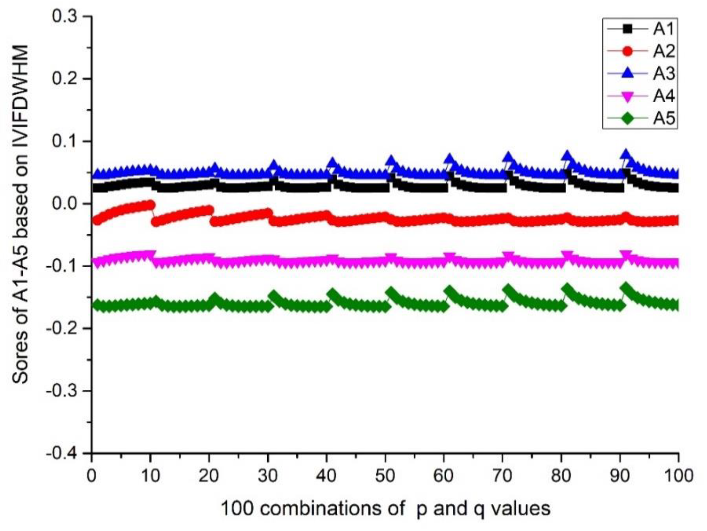
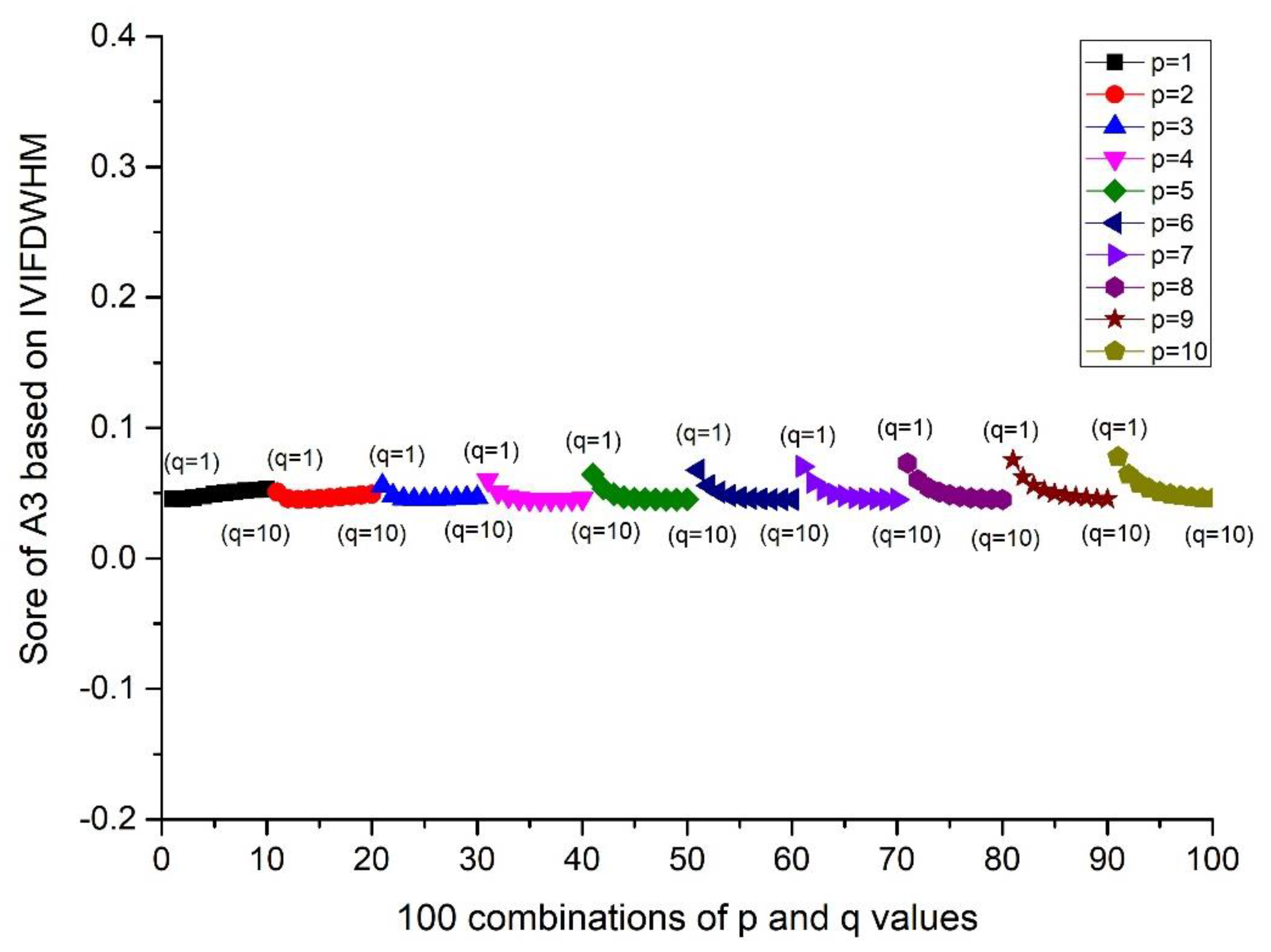
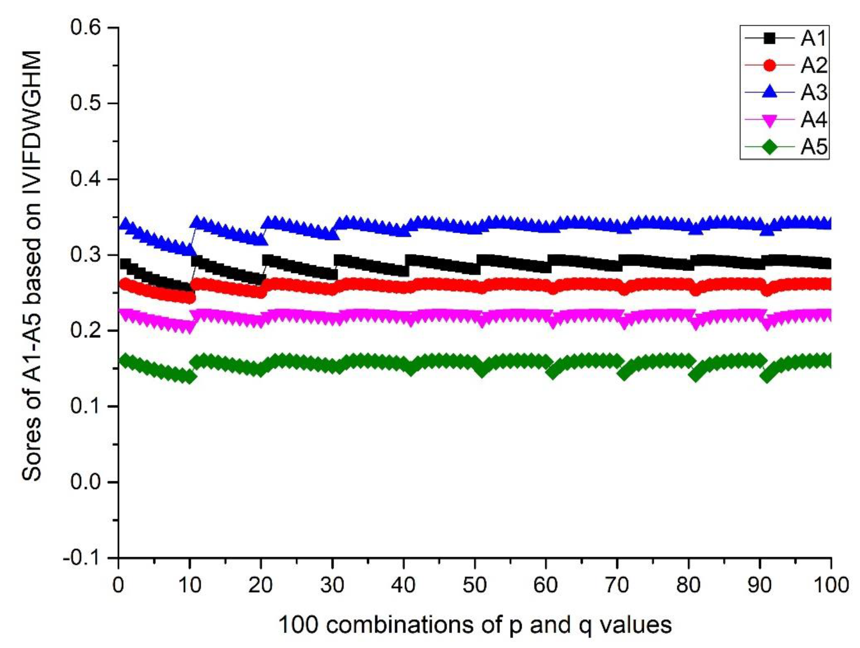
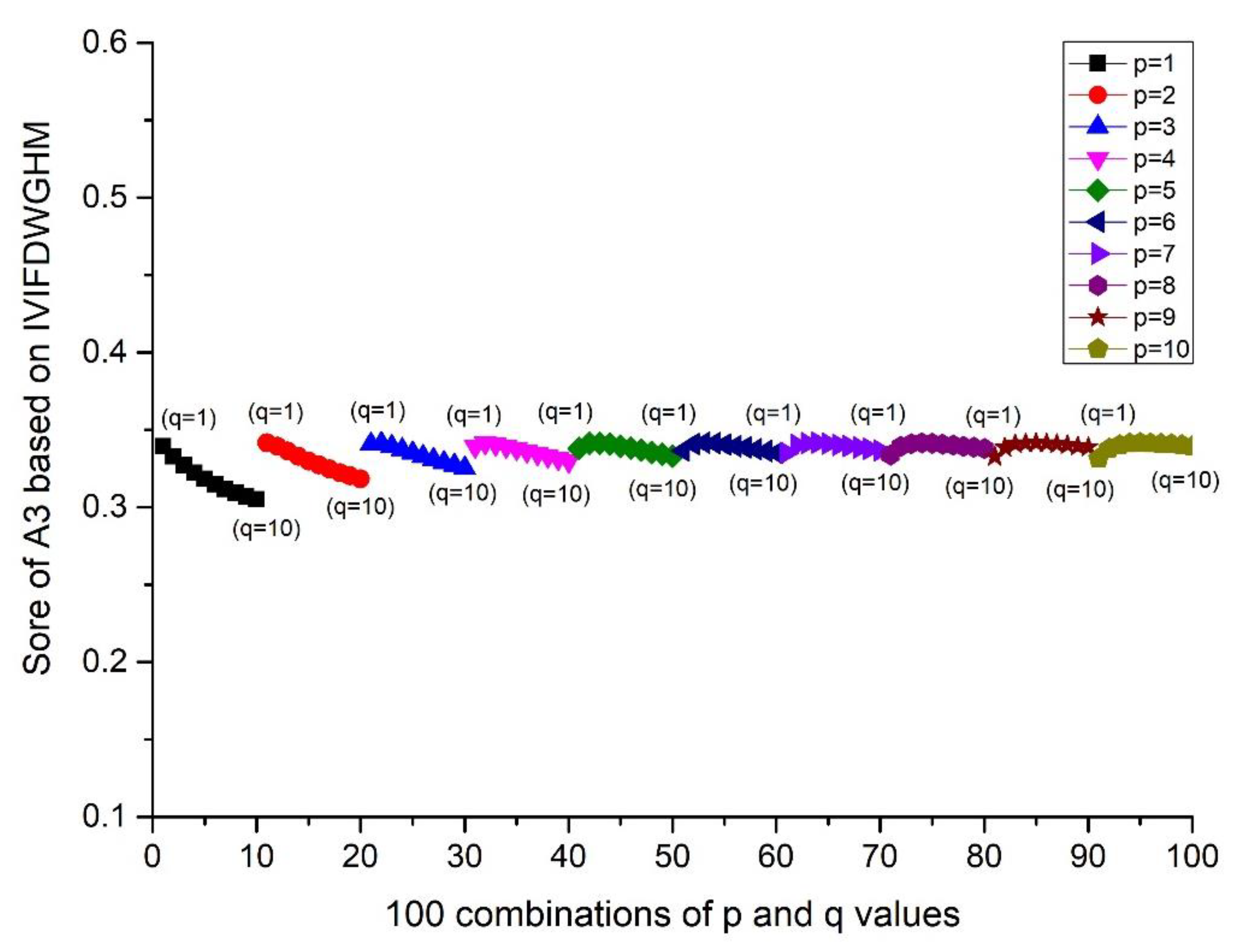
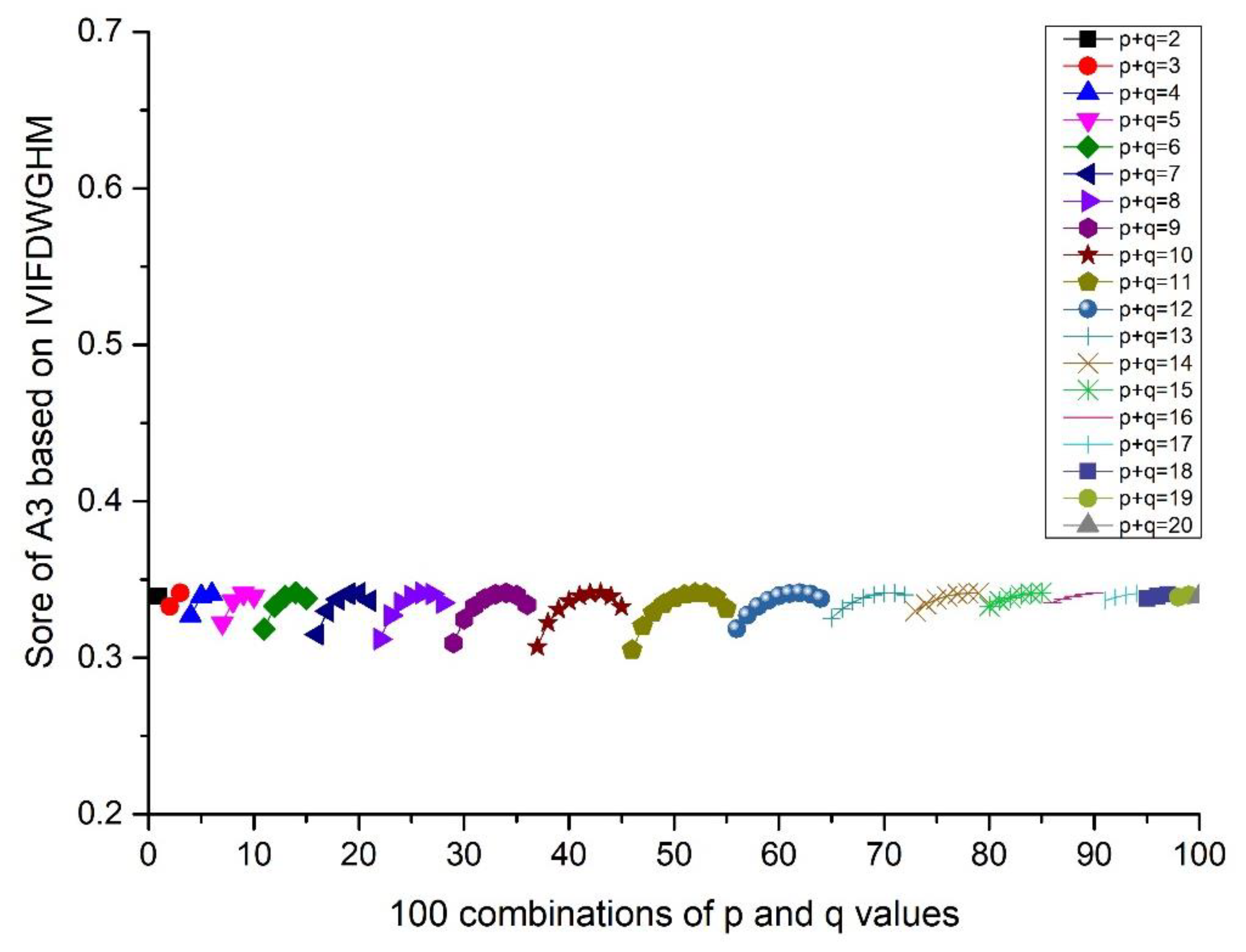
4.2. Influence Analysis

The proposed methods have two independent parameters, $p$ and $q$, which play an important role in the calculation of the results. Hence, different score values and orders may be derived when $p$ and $q$ change. Furthermore, the integer values of $p$ and $q$ in the range of 1–10 usually receive more attention in practical applications. We investigated the influences of $p$ and $q$ on the decision-making from the results of the IVIFWDHM operator and the IVIFWDGHM operator. Firstly, the different $p$ and $q$ are assigned in a certain order with $\left(p_i,q_j\right)$ $\left(i=1,2,\cdots ,10;j=1,2,\dots ,10\right)$. The scores and ranking results of $A_i\left(i=1,2,3,4,5\right)$ are given in Figure 1 and Figure 4. Then, the influence of $q$ (or $p$) on the score is investigated from the result of $A_3$, when the $p$ value is fixed and $q$ changes from 1 to 10. Details can be found in Figure 2 and Figure 5. Moreover, the influence of $p+q$ on the score is investigated from the result of $A_3$, when $p+q$ changes from 2 to 20. Details can be found in Figure 3 and Figure 6.

According to Figure 1 and Figure 4, we can conclude that different scores of alternatives can be derived according to different $p$ and $q$. The differences between the maximum and minimum scores of A₁ to A₅ from the IVIFWDHM operator are 0.0243, 0.0265, 0.0326, 0.0132 and 0.0296, respectively, and the differences between the maximum and minimum scores of A₁ to A₅ from the IVIFWDHM operator are 0.0385, 0.0187, 0.0365, 0.0164 and 0.0212, respectively. It can be seen that the fluctuation range of the scores from the IVIFWDHM operator and the IVIFWDGHM operator are small. Different $p$ and $q$ values have little effect on the scores of the two methods for A₁ to A₅, so the scores of IVIFWDHM operator and IVIFWDGHM operator are stable for different $p$ and $q$ values. However, A₁ to A₅ show some variation rules for different $p$ and $q$ values. The following takes the scores of A₃ from the IVIFWDHM operator and the IVIFWDGHM operator as examples to show the variation rules: (1) For the IVIFWDHM operator, Figure 2 shows that when the $p$ value is fixed and the $q$ value changes from 1 to 10, the fluctuation trend of the score is more complex, most of which has a decreasing trend; Figure 3 shows that when the $p+q$ value changes from 2 to 20, the fluctuation range increases first and then decreases, and reaches its maximum when the $p+q$ value equals 11, then the fluctuation range is from 0.0450 to 0.0776 when $p+q$ value equals 11, which is the same as that of the scores about the 100 combinations of A₃. But the average score of each group has little difference under a certain $p+q$ value, the difference between the maximum average score and the minimum average score is 0.0070, while the fluctuation range is from 0.0458 to 0.0528, which is only 21.45% of the amplitude of the fluctuation range about the 100 combinations of A₃. (2) For the IVIFWDGHM operator, Figure 5 shows that when the $p$ value is fixed and the $q$ value changes from 1 to 10, the fluctuation trend of the score is more complex, and the decreasing trend is dominant; Figure 6 shows that when $p+q$ value changes from 2 to 20, the fluctuation range increases first and then decreases, and reaches its maximum when $p+q$ value equals 11, then the fluctuation range is from 0.3050 to 0.3414, which is the same as that of the scores about the 100 combinations of A₃. But the average score of each group has little difference under a certain $p+q$ value, the difference between the maximum average score and the minimum average score is 0.0075, while the fluctuation range is from 0.3050 to 0.3414, which is only 20.46% of the amplitude of the fluctuation range about the 100 combinations of A₃.

In this section, the influence of $p$ and $q$ on the scores are investigated for the IVIFWDHM operator and the IVIFWDGHM operator. Although results illustrate the regularity of the proposed method for the different $p$ and $q$, different $p$ and $q$ values have little effect on the score values for the two methods_. So the scores of the IVIFWDHM operator and the IVIFWDGHM operator are stable for different $p$ and $q$ values. When the scores of the subjects are similar, it is likely that the ranking of evaluation will change, but when there is a certain gap in the scores of the subjects, the ranking of evaluation will not change. Thus, the proposed methods are sufficient to solve practical MADM. Furthermore, the proposed methods show high robustness for information fusion in MADM.

4.3. Comparative Analysis

We compare the IVIFWDHM and IVIFWDGHM operators with the IVIFWA operator [64], the IVIFWG operator [4], the gray relational analysis method [47] and correlation coefficient [76]. The results are given in

Table 5. Order of the tourism scenic spots.

Methods	Order
IVIFWA operator [64]	A3 > A1 > A4 > A2 > A5
IVIFWG operator [4]	A3 > A1 > A2 > A4 > A5
Gray Relational Analysis Method [47]	A3 > A5 > A1 > A2 > A4
Correlation Coefficient [76]	A3 > A1 > A2 > A4 > A5

.

From the above analysis, we get the same best forest ecological tourism demonstration areas, while the four methods’ orders are slightly different. However, the existing methods with IVIFNs don’t consider the interrelationship among the arguments. Our proposed IVIFWDHM and IVIFWDGHM operators consider the interrelationship among aggregated arguments.

Xu and Chen [77] defined some Bonferroni mean for aggregating the IVIFNs. However, these Bonferroni mean for aggregating the IVIFNs only consider the relationship information between two arguments, and do not consider the relationship information among more than two arguments.

5. Conclusions

Traditional mass tourism attaches much importance to economic profits, while it is intended to meet the aesthetic needs of people. However, behind the high-speed development of tourism, there are difficulties in solving the relationship between man and the nature with the problems aroused in the ecological environment and resources in tourist spots. Eco-tourism is the result of advocating a harmonious coexistence between human beings and the nature, which also indicates both a new concept of tourism, and the ecological conceptions reflected in recreation behaviors of tourists. It advocates such ideas as the harmonious coexistence of man and the nature, and enjoying the nature without destroying the environment, which essentially derive from a concept of humans going back to the nature. Superficially, it comes from people’s attention to “the exterior” of traditional mass tourism, while philosophically, it suggests people’s awakening to environmental ethics. Tourist theories are becoming more mature with a change of paradigm, in which tourism is developing from the activities of a privileged minority, to a popular mass behavior, observed at present. Essentially, we perceive eco-tourism to be a kind of ecological culture based on the recognition of man’s relationship with the nature, and, that we have entered a new tourism paradigm under the guidance of eco-ethics. Furthermore, it reflects on the ideas of the traditional man-oriented mass tourism and corrects people’s misunderstanding about tourist resources and the ecological environment. In this paper, we investigated MADM with IVIFNs. Then, we utilized HM and Dombi operations to design some HM operators with IVIFNs: IVIFDHM operator, IVIFWDHM operator, IVIFDGHM operator and IVIFWDGHM operator. The main characteristic of these proposed operators were studied. Then, we employed the IVIFWDHM and IVIFWDGHM operators to propose two models for MADM problems with IVIFNs. Finally, a real experimental case for evaluating the ecological value of forest ecological tourism demonstration area was used to show the developed approach. In the subsequent studies, the extension and application of IVIFNs need to be studied in many other uncertain environments [78,79,80,81,82,83,84] and other applications [85,86,87,88,89,90].

References

1. Atanassov, K.T. More on intuitionistic fuzzy-sets. Fuzzy Sets Syst. 1989, 33, 37–45. [Google Scholar] [CrossRef]
2. Atanassov, K.T.; Gargov, G.K. Intuitionistic Fuzzy-Logic. Dokl. Na Bolg. Akad. Na Nauk. 1990, 43, 9–12. [Google Scholar]
3. Xu, Z.S. On correlation measures of intuitionistic fuzzy sets. In Proceedings of the 7th International Conference on Intelligent Data Engineering and Automated Learning, Burgos, Spain, 20–23 September 2006; pp. 16–24. [Google Scholar]
4. Xu, Z.S.; Yager, R.R. Some geometric aggregation operators based on intuitionistic fuzzy sets. Int. J. Gen. Syst. 2006, 35, 417–433. [Google Scholar] [CrossRef]
5. Xu, Z.S. Some similarity measures of intuitionistic fuzzy sets and their applications to multiple attribute decision making. Fuzzy Optim. Decis. Mak. 2007, 6, 109–121. [Google Scholar] [CrossRef]
6. Li, Z.X.; Gao, H.; Wei, G.W. Methods for Multiple Attribute Group Decision Making Based on Intuitionistic Fuzzy Dombi Hamy Mean Operators. Symmetry 2018, 10, 574. [Google Scholar] [CrossRef] [Green Version]
7. Deng, X.M.; Wang, J.; Wei, G.W.; Lu, M. Models for Multiple Attribute Decision Making with Some 2-Tuple Linguistic Pythagorean Fuzzy Hamy Mean Operators. Mathematics 2018, 6, 236. [Google Scholar] [CrossRef] [Green Version]
8. Li, Z.X.; Wei, G.W.; Gao, H. Methods for Multiple Attribute Decision Making with Interval-Valued Pythagorean Fuzzy Information. Mathematics 2018, 6, 228. [Google Scholar] [CrossRef] [Green Version]
9. Li, Z.X.; Wei, G.W.; Lu, M. Pythagorean Fuzzy Hamy Mean Operators in Multiple Attribute Group Decision Making and Their Application to Supplier Selection. Symmetry 2018, 10, 205. [Google Scholar] [CrossRef] [Green Version]
10. Wu, S.J.; Wang, J.; Wei, G.W.; Wei, Y. Research on Construction Engineering Project Risk Assessment with Some 2-Tuple Linguistic Neutrosophic Hamy Mean Operators. Sustainability 2018, 10, 1536. [Google Scholar] [CrossRef] [Green Version]
11. Xu, Z.S. Intuitionistic fuzzy aggregation operators. IEEE Trans. Fuzzy Syst. 2007, 15, 1179–1187. [Google Scholar]
12. Atanassov, K.; Gargov, G. Interval valued intuitionistic fuzzy-sets. Fuzzy Sets Syst. 1989, 31, 343–349. [Google Scholar] [CrossRef]
13. Xu, Z.S.; Chen, J. On geometric aggregation ove interval-valued intuitionistic fuzzy information. In Proceedings of the Fourth International Conference on Fuzzy Systems and Knowledge Discovery (FSKD 2007), Haikou, China, 24–27 August 2007. [Google Scholar]
14. Wu, L.P.; Wei, G.W.; Gao, H.; Wei, Y. Some Interval-Valued Intuitionistic Fuzzy Dombi Hamy Mean Operators and Their Application for Evaluating the Elderly Tourism Service Quality in Tourism Destination. Mathematics 2018, 6, 294. [Google Scholar] [CrossRef] [Green Version]
15. Yu, D.J.; Wu, Y.Y.; Lu, T. Interval-valued intuitionistic fuzzy prioritized operators and their application in group decision making. Knowle. Based Syst. 2012, 30, 57–66. [Google Scholar] [CrossRef]
16. Gao, H.; Wei, G.W.; Huang, Y.H. Dual Hesitant Bipolar Fuzzy Hamacher Prioritized Aggregation Operators in Multiple Attribute Decision Making. IEEE Access 2018, 6, 11508–11522. [Google Scholar] [CrossRef]
17. Wei, G.; Wei, Y. Some single-valued neutrosophic dombi prioritized weighted aggregation operators in multiple attribute decision making. J. Intell. Fuzzy Syst. 2018, 35, 2001–2013. [Google Scholar] [CrossRef]
18. Yager, R.R. The power average operator. IEEE Trans. Syst. Man Cybern. Part A 2001, 31, 724–731. [Google Scholar] [CrossRef]
19. Xu, Z.S.; Yager, R.R. Power-Geometric operators and their use in group decision making. IEEE Trans. Fuzzy Syst. 2010, 18, 94–105. [Google Scholar]
20. Chen, T.Y. An interval-valued intuitionistic fuzzy permutation method with likelihood-based preference functions and its application to multiple criteria decision analysis. Appl. Soft Comput. 2016, 42, 390–409. [Google Scholar] [CrossRef]
21. Wei, G.W. Some induced geometric aggregation operators with intuitionistic fuzzy information and their application to group decision making. Appl. Soft Comput. 2010, 10, 423–431. [Google Scholar] [CrossRef]
22. Liu, P.D.; Teng, F. Multiple Criteria Decision Making Method based on Normal Interval-Valued Intuitionistic Fuzzy Generalized Aggregation Operator. Complexity 2016, 21, 277–290. [Google Scholar] [CrossRef]
23. Dugenci, M. A new distance measure for interval valued intuitionistic fuzzy sets and its application to group decision making problems with incomplete weights information. Appl. Soft Comput. 2016, 41, 120–134. [Google Scholar] [CrossRef]
24. Nguyen, H. A new interval-valued knowledge measure for interval-valued intuitionistic fuzzy sets and application in decision making. Exp. Syst. Appl. 2016, 56, 143–155. [Google Scholar] [CrossRef]
25. Sudharsan, S.; Ezhilmaran, D. Weighted arithmetic average operator based on interval-valued intuitionistic fuzzy values and their application to multi criteria decision making for investment. J. Inform. Optim. Sci. 2016, 37, 247–260. [Google Scholar] [CrossRef]
26. Dammak, F.; Baccour, L.; Ayed, A.B.; Alimi, A.M. ELECTRE Method Using Interval-Valued Intuitionistic Fuzzy Sets and Possibility Theory for Multi-Criteria Decision Making Problem Resolution. In Proceedings of the 2017 IEEE International Conference on Fuzzy Systems (FUZZ-IEEE), Naples, Italy, 9–12 July 2017. [Google Scholar]
27. Opricovic, S.; Tzeng, G.H. Extended VIKOR method in comparison with outranking methods. Eur. J. Oper. Res. 2007, 178, 514–529. [Google Scholar] [CrossRef]
28. Garg, H.; Agarwal, N.; Tripathi, A. Some improved interactive aggregation operators under interval-valued intuitionistic fuzzy environment and their application to decision making process. Sci. Iran. 2017, 24, 2581–2604. [Google Scholar] [CrossRef] [Green Version]
29. Liu, P.D.; Li, H.G. Interval-Valued Intuitionistic Fuzzy Power Bonferroni Aggregation Operators and Their Application to Group Decision Making. Cognit. Comput. 2017, 9, 494–512. [Google Scholar] [CrossRef]
30. Deng, X.M.; Wei, G.W.; Gao, H.; Wang, J. Models for Safety Assessment of Construction Project With Some 2-Tuple Linguistic Pythagorean Fuzzy Bonferroni Mean Operators. IEEE Access 2018, 6, 52105–52137. [Google Scholar] [CrossRef]
31. Tang, X.Y.; Wei, G.W. Models for Green Supplier Selection in Green Supply Chain Management With Pythagorean 2-Tuple Linguistic Information. IEEE Access 2018, 6, 18042–18060. [Google Scholar] [CrossRef]
32. Wang, J.; Wei, G.W.; Wei, Y. Models for Green Supplier Selection with Some 2-Tuple Linguistic Neutrosophic Number Bonferroni Mean Operators. Symmetry 2018, 10, 131. [Google Scholar] [CrossRef] [Green Version]
33. Xu, Z.S.; Yager, R.R. Intuitionistic Fuzzy Bonferroni Means. IEEE Trans. Syst. Man Cybern. Part B Cybern. 2011, 41, 568–578. [Google Scholar]
34. Wang, S.F. Interval-valued intuitionistic fuzzy Choquet integral operators based on Archimedean t-norm and their calculations. J. Comput. Anal. Appl. 2017, 23, 703–712. [Google Scholar]
35. Garg, H.; Arora, R. A nonlinear-programming methodology for multi-attribute decision-making problem with interval-valued intuitionistic fuzzy soft sets information. Appl. Intell. 2018, 48, 2031–2046. [Google Scholar] [CrossRef]
36. Hashemi, H.; Bazargan, J.; Mousavi, S.M.; Vandani, B. An extended compromise ratio model with an application to reservoir flood control operation under an interval-valued intuitionistic fuzzy environment. Appl. Math. Model. 2014, 38, 3495–3511. [Google Scholar] [CrossRef]
37. Kim, T.; Sotirova, E.; Shannon, A.; Atanassova, V.; Atanassov, K.; Jang, L.C. Interval Valued Intuitionistic Fuzzy Evaluations for Analysis of a Student’s Knowledge in University e-Learning Courses. Int. J. Fuzzy Logic Intell. Syst. 2018, 18, 190–195. [Google Scholar] [CrossRef] [Green Version]
38. Liu, Z.M.; Teng, F.; Liu, P.D.; Ge, Q. Interval-valued intuitionistic fuzzy power maclaurin symmetric mean aggregation operators and their application to multiple attribute group decision-making. Int. J. Uncertain. Quantif. 2018, 8, 211–232. [Google Scholar] [CrossRef]
39. Wei, G.W.; Garg, H.; Gao, H.; Wei, C. Interval-Valued Pythagorean Fuzzy Maclaurin Symmetric Mean Operators in Multiple Attribute Decision Making. IEEE Access 2018, 6, 67866–67884. [Google Scholar] [CrossRef]
40. Wei, G.W.; Lu, M. Pythagorean Fuzzy Maclaurin Symmetric Mean Operators in Multiple Attribute Decision Making. Int. J. Intell. Syst. 2018, 33, 1043–1070. [Google Scholar] [CrossRef]
41. Bai, K.Y.; Zhu, X.M.; Wang, J.; Zhang, R.T. Some Partitioned Maclaurin Symmetric Mean Based on q-Rung Orthopair Fuzzy Information for Dealing with Multi-Attribute Group Decision Making. Symmetry 2018, 10, 383. [Google Scholar] [CrossRef] [Green Version]
42. Garg, H. A new generalized improved score function of interval-valued intuitionistic fuzzy sets and applications in expert systems. Appl. Soft Comput. 2016, 38, 988–999. [Google Scholar] [CrossRef]
43. Xia, M.M. Interval-valued intuitionistic fuzzy matrix games based on Archimedean t-conorm and t-norm. Int. J. Gen. Syst. 2018, 47, 278–293. [Google Scholar] [CrossRef]
44. Chen, T.Y. IVIF-PROMETHEE outranking methods for multiple criteria decision analysis based on interval-valued intuitionistic fuzzy sets. Fuzzy Optim. Decis. Mak. 2015, 14, 173–198. [Google Scholar] [CrossRef]
45. Chen, S.M.; Han, W.H. Multiattribute decision making based on nonlinear programming methodology, particle swarm optimization techniques and interval-valued intuitionistic fuzzy values. Inform. Sci. 2019, 471, 252–268. [Google Scholar] [CrossRef]
46. Liu, B.S.; Chen, Y.; Shen, Y.H.; Sun, H.; Xu, X.H. A complex multi-attribute large-group decision making method based on the interval-valued intuitionistic fuzzy principal component analysis model. Soft Comput. 2014, 18, 2149–2160. [Google Scholar] [CrossRef]
47. Wei, G.W. Gray relational analysis method for intuitionistic fuzzy multiple attribute decision making. Exp. Syst. Appl. 2011, 38, 11671–11677. [Google Scholar] [CrossRef]
48. Chen, T.Y. The Inclusion-Based LINMAP Method for Multiple Criteria Decision Analysis Within an Interval-Valued Atanassov’s Intuitionistic Fuzzy Environment. Int. J. Inform. Technol. Decis. Mak. 2014, 13, 1325–1360. [Google Scholar] [CrossRef]
49. Cuong, B.C.; Kreinovich, V. Picture Fuzzy Sets—A new concept for computational intelligence problems. In Proceedings of the 2013 Third World Congress on Information and Communication Technologies (WICT 2013), Hanoi, Vietnam, 15–18 December 2013. [Google Scholar]
50. Singh, P. Correlation coefficients for picture fuzzy sets. J. Intell. Fuzzy Syst. 2015, 28, 591–604. [Google Scholar] [CrossRef]
51. Thong, N.T.; Son, L.H. HIFCF: An effective hybrid model between picture fuzzy clustering and intuitionistic fuzzy recommender systems for medical diagnosis. Exp. Syst. Appl. 2015, 42, 3682–3701. [Google Scholar] [CrossRef]
52. Wang, R.; Wang, J.; Gao, H.; Wei, G.W. Methods for MADM with Picture Fuzzy Muirhead Mean Operators and Their Application for Evaluating the Financial Investment Risk. Symmetry 2019, 11, 6. [Google Scholar] [CrossRef] [Green Version]
53. Yager, R.R.; Abbasov, A.M. Pythagorean Membership Grades, Complex Numbers, and Decision Making. Int. J. Intell. Syst. 2013, 28, 436–452. [Google Scholar] [CrossRef]
54. Wei, G.W. Pythagorean fuzzy Hamacher Power aggregation operators in multiple attribute decision making. Fundam. Inform. 2019, 166, 57–85. [Google Scholar] [CrossRef]
55. Gao, H. Pythagorean fuzzy Hamacher Prioritized aggregation operators in multiple attribute decision making. J. Intell. Fuzzy Syst. 2018, 35, 2229–2245. [Google Scholar] [CrossRef]
56. Yager, R. Generalized Orthopair Fuzzy Sets. IEEE Trans. Fuzzy Syst. 2017, 25, 1222–1230. [Google Scholar] [CrossRef]
57. Liu, P.D.; Liu, J.L. Some q-Rung Orthopai Fuzzy Bonferroni Mean Operators and Their Application to Multi-Attribute Group Decision Making. Int. J. Intell. Syst. 2018, 33, 315–347. [Google Scholar] [CrossRef]
58. Liu, P.D.; Wang, P. Some q-Rung Orthopair Fuzzy Aggregation Operators and their Applications to Multiple-Attribute Decision Making. Int. J. Intell. Syst. 2018, 33, 259–280. [Google Scholar] [CrossRef]
59. Wei, G.W.; Wei, C.; Wang, J.; Gao, H.; Wei, Y. Some q-rung orthopair fuzzy maclaurin symmetric mean operators and their applications to potential evaluation of emerging technology commercialization. Int. J. Intell. Syst. 2019, 34, 50–81. [Google Scholar] [CrossRef]
60. Ye, J. Multiple Attribute Decision-Making Method Using Correlation Coefficients of Normal Neutrosophic Sets. Symmetry 2017, 9, 80. [Google Scholar] [CrossRef] [Green Version]
61. Dombi, J. A general-class of fuzzy operators, the demorgan class of fuzzy operators and fuzziness measures induced by fuzzy operators. Fuzzy Sets Syst. 1982, 8, 149–163. [Google Scholar] [CrossRef]
62. Dombi, J.; Gyorbiro, N. Addition of sigmoid-shaped fuzzy intervals using the Dombi operator and infinite sum theorems. Fuzzy Sets Syst. 2006, 157, 952–963. [Google Scholar] [CrossRef]
63. Dombi, J. The Generalized Dombi Operator Family and the Multiplicative Utility Function. In Soft Computing Based Modeling in Intelligent Systems; Balas, V.E., Fodor, J., VarkonyiKoczy, A.R., Eds.; Springer: London, UK, 2009; pp. 115–131. [Google Scholar]
64. Xu, Z.S.; Yager, R.R. Dynamic intuitionistic fuzzy multi-attribute decision making. Int. J. Approx. Reason. 2008, 48, 246–262. [Google Scholar] [CrossRef] [Green Version]
65. Hara, Y.; Uchiyama, M.; Takahasi, S.E. A refinement of various mean inequalities. J. Inequal. Appl. 1998, 2, 387–395. [Google Scholar] [CrossRef]
66. Tang, X.Y.; Wei, G.W. Multiple Attribute Decision-Making with Dual Hesitant Pythagorean Fuzzy Information. Cognit. Comput. 2019, 11, 193–211. [Google Scholar] [CrossRef]
67. Tang, X.Y.; Wei, G.W.; Gao, H. Models for Multiple Attribute Decision Making with Interval-Valued Pythagorean Fuzzy Muirhead Mean Operators and Their Application to Green Suppliers Selection. Informatica 2019, 30, 153–186. [Google Scholar] [CrossRef]
68. Teng, F.; Liu, P. Multiple-Attribute Group Decision-Making Method Based on the Linguistic Intuitionistic Fuzzy Density Hybrid Weighted Averaging Operator. Int. J. Fuzzy Syst. 2019, 21, 213–231. [Google Scholar] [CrossRef]
69. Wei, G.W.; Wei, C.; Wu, J.; Wang, H.J. Supplier Selection of Medical Consumption Products with a Probabilistic Linguistic MABAC Method. Int. J. Environ. Res. Public Health 2019, 16, 5082. [Google Scholar] [CrossRef] [PubMed] [Green Version]
70. He, T.T.; Wei, G.W.; Lu, C.W.J.P.; Lin, R. Pythagorean 2-Tuple Linguistic Taxonomy Method for Supplier Selection in Medical Instrument Industries. Int. J. Environ. Res. Public Health 2019, 16, 4875. [Google Scholar] [CrossRef] [PubMed] [Green Version]
71. He, T.T.; Wei, G.W.; Lu, J.P.; Wei, C.; Lin, R. Pythagorean 2-Tuple Linguistic VIKOR Method for Evaluating Human Factors in Construction Project Management. Mathematics 2019, 7, 1149. [Google Scholar] [CrossRef] [Green Version]
72. Lu, J.P.; Tang, X.Y.; Wei, G.W.; Wei, C.; Wei, Y. Bidirectional project method for dual hesitant Pythagorean fuzzy multiple attribute decision-making and their application to performance assessment of new rural construction. Int. J. Intell. Syst. 2019, 34, 1920–1934. [Google Scholar] [CrossRef]
73. Lu, J.P.; Wei, C.; Wu, J.; Wei, G.W. TOPSIS Method for Probabilistic Linguistic MAGDM with Entropy Weight and Its Application to Supplier Selection of New Agricultural Machinery Products. Entropy 2019, 21, 953. [Google Scholar] [CrossRef] [Green Version]
74. Wei, G.W. 2-tuple intuitionistic fuzzy linguistic aggregation operators in multiple attribute decision making. Iran. J. Fuzzy Syst. 2019, 16, 159–174. [Google Scholar]
75. Wei, G.W. The generalized dice similarity measures for multiple attribute decision making with hesitant fuzzy linguistic information. Econ. Res. Ekonomska Istrazivanja 2019, 32, 1498–1520. [Google Scholar] [CrossRef] [Green Version]
76. Wei, G.W.; Wang, H.J.; Lin, R. Application of correlation coefficient to interval-valued intuitionistic fuzzy multiple attribute decision-making with incomplete weight information. Knowl. Inform. Syst. 2011, 26, 337–349. [Google Scholar] [CrossRef]
77. Xu, Z.S.; Chen, Q. A multi-criteria decision making procedure based on interval-valued intuitionistic fuzzy bonferroni means. J. Syst. Sci. Syst. Eng. 2011, 20, 217–228. [Google Scholar] [CrossRef]
78. Wang, J.; Gao, H.; Wei, G.W. Some 2-tuple linguistic neutrosophic number Muirhead mean operators and their applications to multiple attribute decision making. J. Exp. Theor. Artif. Intell. 2019, 31, 409–439. [Google Scholar] [CrossRef]
79. Zehforoosh, Y. Evaluation of a mushroom shape CPW-fed antenna with triple band-notched characteristics for UWB applications based on multiple attribute decision making. Analog Integr. Circ. Sig. Process. 2019, 98, 385–393. [Google Scholar] [CrossRef]
80. Gao, H.; Ran, L.G.; Wei, G.W.; Wei, C.; Wu, J. VIKOR Method for MAGDM Based on Q-Rung Interval-Valued Orthopair Fuzzy Information and Its Application to Supplier Selection of Medical Consumption Products. Int. J. Environ. Res. Public Health 2020, 17, 525. [Google Scholar] [CrossRef] [Green Version]
81. Deng, X.M.; Gao, H. TODIM method for multiple attribute decision making with 2-tuple linguistic Pythagorean fuzzy information. J. Intell. Fuzzy Syst. 2019, 37, 1769–1780. [Google Scholar] [CrossRef]
82. Gao, H.; Lu, M.; Wei, Y. Dual hesitant bipolar fuzzy hamacher aggregation operators and their applications to multiple attribute decision making. J. Intell. Fuzzy Syst. 2019, 37, 5755–5766. [Google Scholar] [CrossRef]
83. Li, Z.X.; Lu, M. Some novel similarity and distance and measures of Pythagorean fuzzy sets and their applications. J. Intell. Fuzzy Syst. 2019, 37, 1781–1799. [Google Scholar] [CrossRef]
84. Lu, J.P.; Wei, C. TODIM method for Performance Appraisal on Social-Integration-based Rural Reconstruction with Interval-Valued Intuitionistic Fuzzy Information. J. Intell. Fuzzy Syst. 2019, 37, 1731–1740. [Google Scholar] [CrossRef]
85. Wei, Y.; Qin, S.; Li, X.; Zhu, S.; Wei, G. Oil price fluctuation, stock market and macroeconomic fundamentals: Evidence from China before and after the financial crisis. Financ. Res. Lett. 2019, 30, 23–29. [Google Scholar] [CrossRef]
86. Choudhary, A.; Nizamuddin, M.; Singh, M.K.; Sachan, V.K. Energy Budget Based Multiple Attribute Decision Making (EB-MADM) Algorithm for Cooperative Clustering in Wireless Body Area Networks. J. Electr. Eng. Technol. 2019, 14, 421–433. [Google Scholar] [CrossRef]
87. He, Y.; Liao, N.; Bi, J.J.; Guo, L.W. Investment decision-making optimization of energy efficiency retrofit measures in multiple buildings under financing budgetary restraint. J. Clean. Prod. 2019, 215, 1078–1094. [Google Scholar] [CrossRef]
88. Wang, J.; Gao, H.; Lu, M. Approaches to strategic supplier selection under interval neutrosophic environment. J. Intell. Fuzzy Syst. 2019, 37, 1707–1730. [Google Scholar] [CrossRef]
89. Wu, L.P.; Gao, H.; Wei, C. VIKOR method for financing risk assessment of rural tourism projects under interval-valued intuitionistic fuzzy environment. J. Intell. Fuzzy Syst. 2019, 37, 2001–2008. [Google Scholar] [CrossRef]
90. Wu, L.P.; Wang, J.; Gao, H. Models for competiveness evaluation of tourist destination with some interval-valued intuitionistic fuzzy Hamy mean operators. J. Intell. Fuzzy Syst. 2019, 36, 5693–5709. [Google Scholar] [CrossRef]
Figure 1. Scores of Ai (i = 1,2,3,4,5) based on the IVIFWDHM operator (λ = 3) for different integer p and q ∈ [1, 10].
Ijerph 17 00829 g001
Figure 2. Score of A3 based on the IVIFWDHM operator (λ = 3) for different p and q ∈ [1, 10] when p is fixed and q changes from 1 to 10.
Ijerph 17 00829 g002
Figure 3. Score of A3 based on the IVIFWDHM operator (λ = 3) for different p and q ∈ [1, 10] when p + q changes from 2 to 20.
Ijerph 17 00829 g003
Figure 4. Scores of Ai (i = 1,2,3,4,5) based on the IVIFWDGHM operator (λ = 3) for different integer p and q ∈ [1, 10].
Ijerph 17 00829 g004
Figure 5. Score of A3 based on the IVIFWDGHM operator (λ = 3) for different p and q ∈ [1, 10] when p is fixed and q changes from 1 to 10.
Ijerph 17 00829 g005
Figure 6. Score of A3 based on the IVIFWDGHM operator (λ = 3) for different p and q ∈ [1, 10] when p + q changes from 2 to 20.
Ijerph 17 00829 g006