
Predicting Physician Consultations for Low Back Pain Using Claims Data and Population-Based Cohort Data—An Interpretable Machine Learning Approach


Abstract
:1. Introduction
2. Materials and Methods
2.1. Data Sources
2.1.1. Study of Health in Pomerania
2.1.2. Claims Data
2.1.3. Record Linkage
2.2. Methods
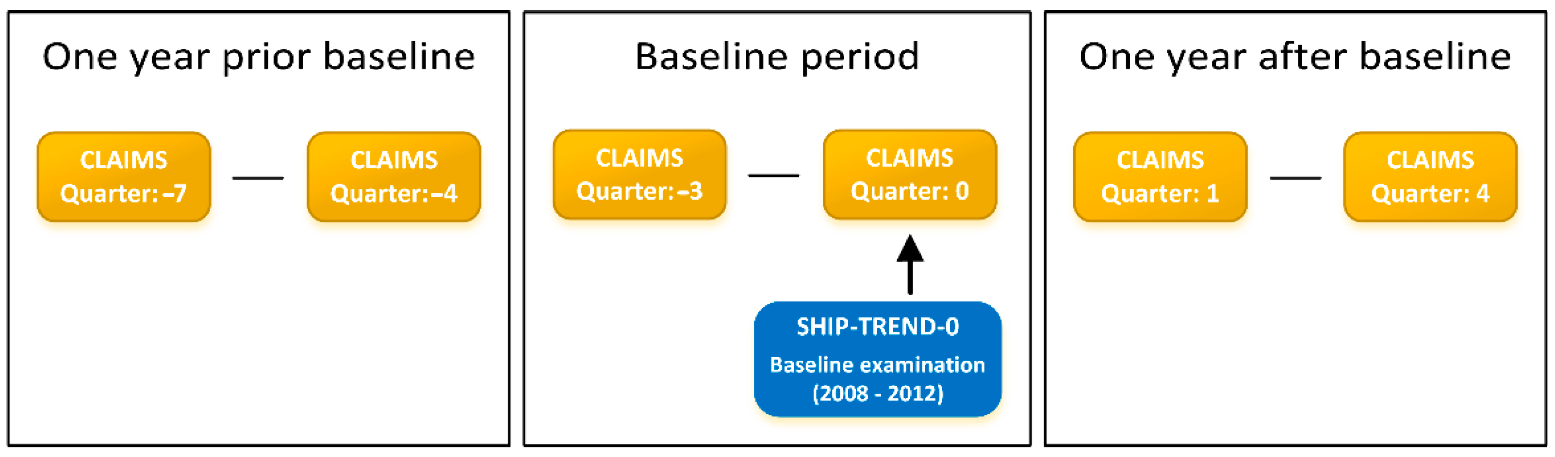
2.2.1. Study Design
2.2.2. Primary Outcome
2.2.3. Candidate Variables
2.2.4. Model Training
2.2.5. Model Evaluation
2.2.6. Missing Data
2.2.7. Comparative Analyses
2.2.8. Subgroup Analyses
3. Results
3.1. Cohort Characteristics
3.2. Best Subset Models
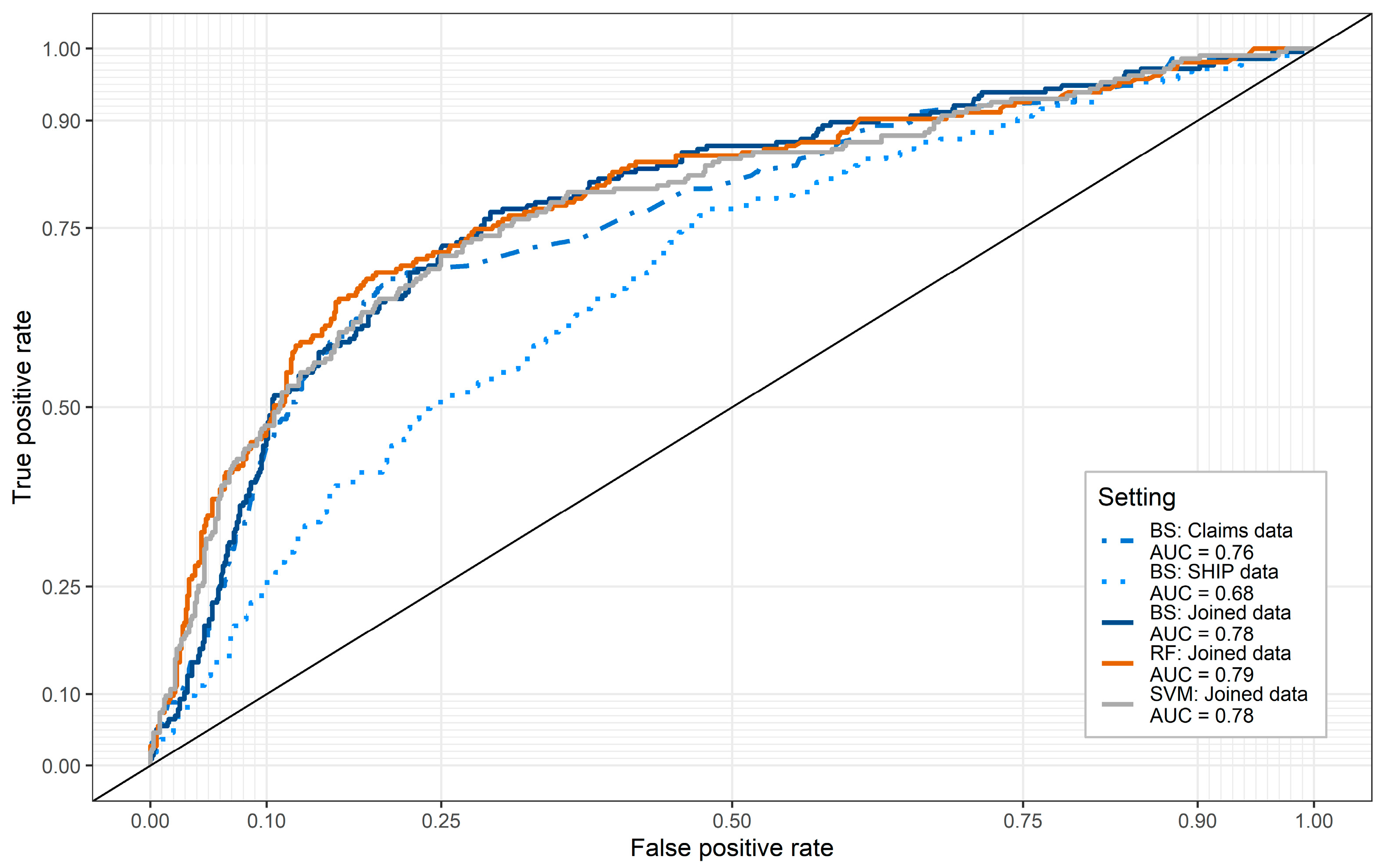
3.3. Predictive Accuracy and Comparative Analyses
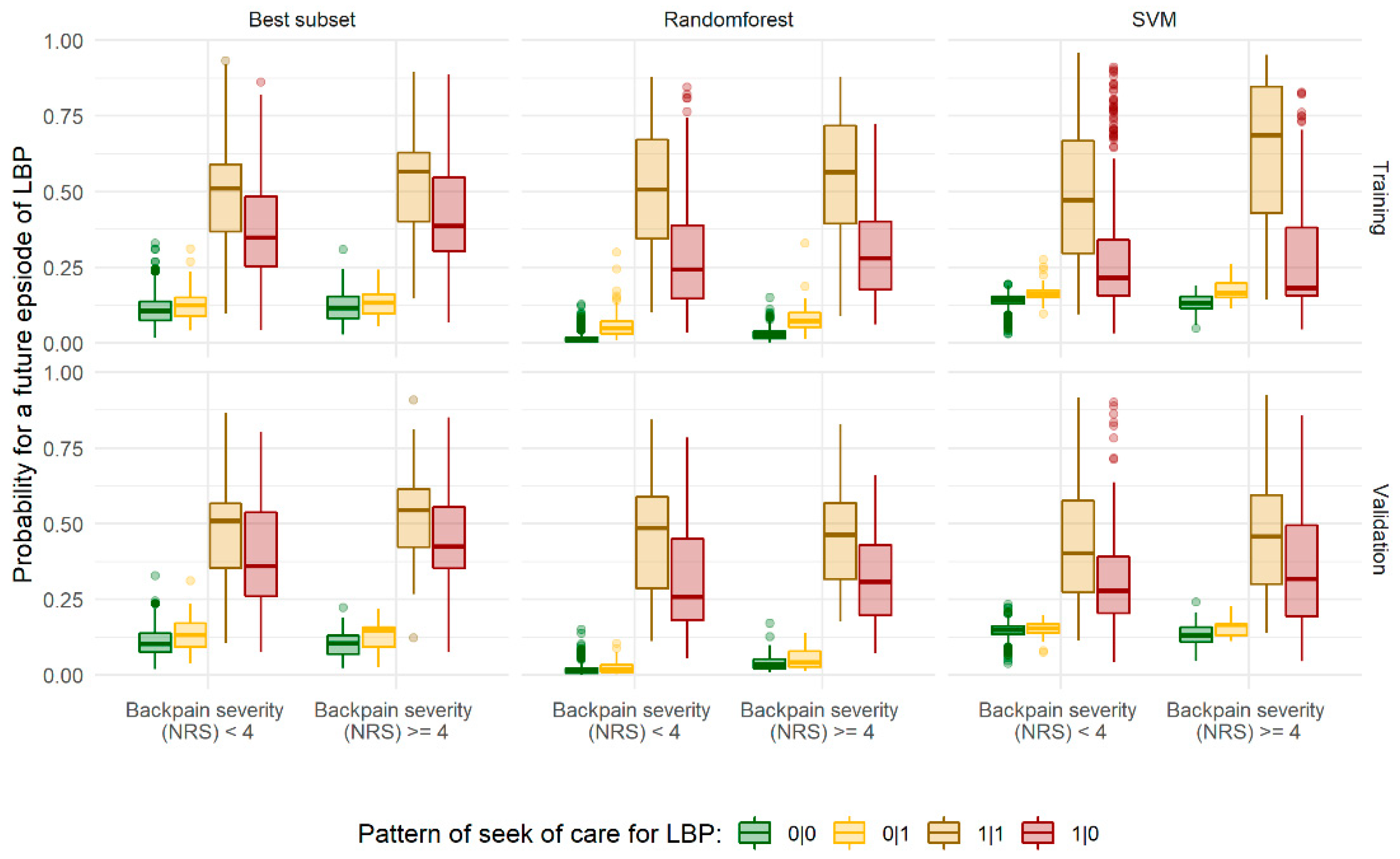
3.4. Subgroup Analyses
4. Discussion
5. Conclusions
Supplementary Materials
Author Contributions
Funding
Institutional Review Board Statement
Informed Consent Statement
Data Availability Statement
Acknowledgments
Conflicts of Interest
References
- Chenot, J.-F.; Greitemann, B.; Kladny, B.; Petzke, F.; Pfingsten, M.; Schorr, S.G. Non-Specific Low Back Pain. Dtsch. Aerzteblatt Online 2017, 114, 883–890. [Google Scholar] [CrossRef] [Green Version]
- Maher, C.; Underwood, M.; Buchbinder, R. Non-specific low back pain. Lancet 2017, 389, 736–747. [Google Scholar] [CrossRef] [Green Version]
- Wenig, C.M.; Schmidt, C.O.; Kohlmann, T.; Schweikert, B. Costs of back pain in Germany. Eur. J. Pain 2009, 13, 280–286. [Google Scholar] [CrossRef] [PubMed]
- Pengel, L.; Herbert, R.D.; Maher, C.; Refshauge, K.M. Acute low back pain: Systematic review of its prognosis. BMJ 2003, 327, 323. [Google Scholar] [CrossRef] [Green Version]
- Hestbaek, L.; Leboeuf-Yde, C.; Manniche, C. Low back pain: What is the long-term course? A review of studies of general patient populations. Eur. Spine J. 2003, 12, 149–165. [Google Scholar] [CrossRef] [PubMed]
- Canizares, M.; Rampersaud, Y.R.; Badley, E.M. Course of Back Pain in the Canadian Population: Trajectories, Predictors, and Outcomes. Arthritis Rheum. 2019, 71, 1660–1670. [Google Scholar] [CrossRef]
- Breiman, L. Random forests. Mach. Learn. 2001, 45, 5–32. [Google Scholar] [CrossRef] [Green Version]
- Weng, S.F.; Reps, J.M.; Kai, J.; Garibaldi, J.M.; Qureshi, N. Can machine-learning improve cardiovascular risk prediction using routine clinical data? PLoS ONE 2017, 12, e0174944. [Google Scholar] [CrossRef] [Green Version]
- Kruppa, J.; Liu, Y.; Diener, H.-C.; Holste, T.; Weimar, C.; König, I.R.; Ziegler, A. Probability estimation with machine learning methods for dichotomous and multicategory outcome: Applications. Biom. J. 2014, 56, 564–583. [Google Scholar] [CrossRef] [PubMed]
- Boulesteix, A.-L.; Schmid, M. Machine learning versus statistical modeling. Biom. J. 2014, 56, 588–593. [Google Scholar] [CrossRef]
- Beale, E.M.L.; Kendall, M.G.; Mann, D.W. The discarding of variables in multivariate analysis. Biometrika 1967, 54, 357–366. [Google Scholar] [CrossRef]
- Hastie, T.; Tibshirani, R.; Tibshirani, R. Best Subset, Forward Stepwise or Lasso? Analysis and Recommendations Based on Extensive Comparisons. Stat. Sci. 2020, 35, 579–592. [Google Scholar] [CrossRef]
- Völzke, H.; Alte, D.; Schmidt, F.; Radke, D.; Lorbeer, R.; Friedrich, N.; Aumann, N.; Lau, K.; Piontek, K.; Born, G.; et al. Cohort Profile: The Study of Health in Pomerania. Int. J. Epidemiol. 2010, 40, 294–307. [Google Scholar] [CrossRef] [Green Version]
- Kroenke, K.; Spitzer, R.L.; Williams, J.B. The PHQ-9: Validity of a brief depression severity measure. J. Gen. Intern. Med. 2001, 16, 606–613. [Google Scholar] [CrossRef] [PubMed]
- Von Korff, M.; Ormel, J.; Keefe, F.J.; Dworkin, S.F. Grading the severity of chronic pain. Pain 1992, 50, 133–149. [Google Scholar] [CrossRef]
- Schmidt, C.O.; Raspe, H.; Pfingsten, M.; Hasenbring, M.I.; Basler, H.D.; Eich, W.; Kohlmann, T. Back Pain in the German Adult Population. Spine 2007, 32, 2005–2011. [Google Scholar] [CrossRef]
- Das Bundesgesundheitsministerium. Das deutsche Gesundheitssystem—Leistungsstark. Sicher. Bewährt. 2020. Available online: https://www.bundesgesundheitsministerium.de/fileadmin/Dateien/5_Publikationen/Gesundheit/Broschueren/200629_BMG_Das_deutsche_Gesundheitssystem_DE.pdf (accessed on 15 November 2021).
- Vatsalan, D.; Christen, P.; Verykios, V.S. A taxonomy of privacy-preserving record linkage techniques. Inf. Syst. 2013, 38, 946–969. [Google Scholar] [CrossRef]
- R Development Core Team. R: A Language and Environment for Statistical Computing; R Foundation for Statistical Computing: Vienna, Austria, 2020. [Google Scholar]
- Jackman, S. pscl: Classes and Methods for R Developed in the Political Science Computational Laboratory. 2020. Available online: http://github.com/atahk/pscl (accessed on 8 August 2021).
- Zeileis, A.; Kleiber, C.; Jackman, S. Regression Models for Count Data inR. J. Stat. Softw. 2008, 27, 1–25. [Google Scholar] [CrossRef] [Green Version]
- Weston, S.; Microsoft Corporation. doParallel: Foreach Parallel Adaptor for the ‘parallel’ Package. 2020. Available online: https://CRAN.R-project.org/package=doParallel (accessed on 8 August 2021).
- University of Greifswald. HPC Brain Cluster. Available online: https://rz.uni-greifswald.de/dienste/allgemein/sonstiges/high-performance-computing/ (accessed on 8 August 2021).
- Broek, J.V.D. A Score Test for Zero Inflation in a Poisson Distribution. Biometrics 1995, 51, 738. [Google Scholar] [CrossRef]
- Friendly, M. vcdExtra: ’vcd’ Extensions and Additions. 2021. Available online: https://CRAN.R-project.org/package=vcdExtra (accessed on 8 August 2021).
- Sundararajan, V.; Henderson, T.; Perry, C.; Muggivan, A.; Quan, H.; Ghali, W.A. New ICD-10 version of the Charlson comorbidity index predicted in-hospital mortality. J. Clin. Epidemiol. 2004, 57, 1288–1294. [Google Scholar] [CrossRef] [PubMed]
- Hofner, B.; Boccuto, L.; Göker, M. Controlling false discoveries in high-dimensional situations: Boosting with stability selection. BMC Bioinform. 2015, 16, 144. [Google Scholar] [CrossRef] [PubMed] [Green Version]
- Mayr, A.; Hofner, B.; Waldmann, E.; Hepp, T.; Meyer, S.; Gefeller, O. An Update on Statistical Boosting in Biomedicine. Comput. Math. Methods Med. 2017, 2017, 6083072. [Google Scholar] [CrossRef] [Green Version]
- Filzmoser, P.; Liebmann, B.; Varmuza, K. Repeated double cross validation. J. Chemom. 2009, 23, 160–171. [Google Scholar] [CrossRef]
- Burnham, K.P.; Anderson, D.R. Multimodel Inference: Understanding AIC and BIC in Model Selection. Sociol. Methods Res. 2004, 33, 261–304. [Google Scholar] [CrossRef]
- Gneiting, T.; Raftery, A.E. Strictly Proper Scoring Rules, Prediction, and Estimation. J. Am. Stat. Assoc. 2007, 102, 359–378. [Google Scholar] [CrossRef]
- Kleiber, C.; Zeileis, A. Visualizing Count Data Regressions Using Rootograms. Am. Stat. 2016, 70, 296–303. [Google Scholar] [CrossRef] [Green Version]
- Sachs, M.C. plotROC: A Tool for Plotting ROC Curves. J. Stat. Softw. 2017, 79, 1–19. [Google Scholar] [CrossRef] [PubMed]
- Van Buuren, S.; Groothuis-Oudshoorn, K. Mice: Multivariate Imputation by Chained Equations in R. J. Stat. Softw. 2011, 45, 1–67. [Google Scholar] [CrossRef] [Green Version]
- Jakobsen, J.C.; Gluud, C.; Wetterslev, J.; Winkel, P. When and how should multiple imputation be used for handling missing data in randomised clinical trials—A practical guide with flowcharts. BMC Med. Res. Methodol. 2017, 17, 162. [Google Scholar] [CrossRef] [Green Version]
- Madley-Dowd, P.; Hughes, R.; Tilling, K.; Heron, J. The proportion of missing data should not be used to guide decisions on multiple imputation. J. Clin. Epidemiol. 2019, 110, 63–73. [Google Scholar] [CrossRef] [Green Version]
- Vapnik, V.; Guyon, I.; Hastie, T. Support vector machines. Mach. Learn. 1995, 20, 273–297. [Google Scholar]
- Bischl, B.; Binder, M.; Lang, M.; Pielok, T.; Richter, J.; Coors, S.; Thomas, J.; Ullmann, T.; Becker, M.; Boulesteix, A.-L. Hyperparameter Optimization: Foundations, Algorithms, Best Practices and Open Challenges. arXiv 2021, arXiv:2107.05847. [Google Scholar]
- Probst, P.; Wright, M.N.; Boulesteix, A. Hyperparameters and tuning strategies for random forest. Wiley Interdiscip. Rev. Data Min. Knowl. Discov. 2019, 9, 1301. [Google Scholar] [CrossRef] [Green Version]
- Hsu, C.-W.; Chang, C.-C.; Lin, C.-J. A Practical Guide to Support Vector Classification (Update 2016). 2003. Available online: https://www.csie.ntu.edu.tw/~cjlin/papers/guide/guide.pdf (accessed on 8 August 2021).
- Meyer, D.; Dimitriadou, E.; Hornik, K.; Weingessel, A.; Leisch, F. Misc Functions of the Department of Statistics, Probability Theory Group (Formerly: E1071). TU Wien. R Package Version 1.7-2: e1071. 2020. Available online: http://packages.renjin.org/package/org.renjin.cran/e1071 (accessed on 8 August 2021).
- Hosmer, D.W., Jr.; Lemeshow, S.; Sturdivant, R.X. Applied Logistic Regression; John Wiley & Sons: Hoboken, NJ, USA, 2013; Volume 398. [Google Scholar]
- Christodoulou, E.; Ma, J.; Collins, G.S.; Steyerberg, E.W.; Verbakel, J.Y.; Van Calster, B. A systematic review shows no performance benefit of machine learning over logistic regression for clinical prediction models. J. Clin. Epidemiol. 2019, 110, 12–22. [Google Scholar] [CrossRef] [PubMed]
- Karran, E.L.; McAuley, J.H.; Traeger, A.C.; Hillier, S.L.; Grabherr, L.; Russek, L.N.; Moseley, G.L. Can screening instruments accurately determine poor outcome risk in adults with recent onset low back pain? A systematic review and meta-analysis. BMC Med. 2017, 15, 24. [Google Scholar] [CrossRef] [Green Version]
- McIntosh, G.; Steenstra, I.; Hogg-Johnson, S.; Carter, T.; Hall, H. Lack of Prognostic Model Validation in Low Back Pain Prediction Studies. Clin. J. Pain 2018, 34, 748–754. [Google Scholar] [CrossRef] [PubMed]
- Chenot, J.-F.; Leonhardt, C.; Keller, S.; Scherer, M.; Donner-Banzhoff, N.; Pfingsten, M.; Basler, H.-D.; Baum, E.; Kochen, M.M.; Becker, A. The impact of specialist care for low back pain on health service utilization in primary care patients: A prospective cohort study. Eur. J. Pain 2008, 12, 275–283. [Google Scholar] [CrossRef] [PubMed]
- Ferreira, M.L.; Machado, G.; Latimer, J.; Maher, C.; Ferreira, P.H.; Smeets, R. Factors defining care-seeking in low back pain—A meta-analysis of population based surveys. Eur. J. Pain 2010, 14, 747.e1–747.e7. [Google Scholar] [CrossRef]
- Unal, I. Defining an Optimal Cut-Point Value in ROC Analysis: An Alternative Approach. Comput. Math. Methods Med. 2017, 2017, 3762651. [Google Scholar] [CrossRef]
- Mukasa, D.; Sung, J. A prediction model of low back pain risk: A population based cohort study in Korea. Korean J. Pain 2020, 33, 153–165. [Google Scholar] [CrossRef]
- Ramond, A.; Bouton, C.; Richard, I.; Roquelaure, Y.; Baufreton, C.; Legrand, E.; Huez, J.-F. Psychosocial risk factors for chronic low back pain in primary care--a systematic review. Fam. Pract. 2010, 28, 12–21. [Google Scholar] [CrossRef] [PubMed] [Green Version]
- Lynch, C.M.; Abdollahi, B.; Fuqua, J.D.; de Carlo, A.R.; Bartholomai, J.A.; Balgemann, R.N.; van Berkel, V.H.; Frieboes, H.B. Prediction of lung cancer patient survival via supervised machine learning classification techniques. Int. J. Med. Inform. 2017, 108, 1–8. [Google Scholar] [CrossRef] [PubMed]
- Paluszynska, A.; Biecek, P.; Jiang, Y.; Jiang, M.Y. Package ‘randomForestExplainer’. 2017. Available online: http://cran.nexr.com/web/packages/randomForestExplainer/randomForestExplainer.pdf (accessed on 8 August 2021).
- Bertsimas, D.; King, A.; Mazumder, R. Best subset selection via a modern optimization lens. Ann. Stat. 2016, 44, 813–852. [Google Scholar] [CrossRef] [Green Version]


| Characteristic | Statutory Insurances | Private Insurances | |
|---|---|---|---|
| Participants with Consent to Linkage | Participants without Consent to Linkage | ||
| N | 3837 | 242 | 341 |
| Age (years) | |||
| Mean (SD) | 52.6 (15.6) | 50.9 (15.3) | 45.2 (12.1) |
| Median [Min, Max] | 53.0 [20.0, 84.0] | 52.5 [23.0, 81.0] | 44.0 [21.0, 78.0] |
| Family status | |||
| Single | 409 (10.7%) | 40 (16.5%) | 36 (10.6%) |
| Married/Partner | 2964 (77.2%) | 170 (70.2%) | 284 (83.3%) |
| Separated | 241 (6.3%) | 24 (9.9%) | 18 (5.3%) |
| Widowed | 211 (5.5%) | 7 (2.9%) | 3 (0.9%) |
| Missing | 12 (0.3%) | 1 (0.4%) | 0 (0%) |
| Job characteristics | |||
| Never working | 27 (0.7%) | 2 (0.8%) | 5 (1.5%) |
| At desktop, not physically | 1129 (29.4%) | 75 (31.0%) | 188 (55.1%) |
| At desktop and physically demanding | 504 (13.1%) | 36 (14.9%) | 64 (18.8%) |
| Not at desktop, not physically | 796 (20.7%) | 49 (20.2%) | 28 (8.2%) |
| Not at desktop but physically demanding | 1220 (31.8%) | 61 (25.2%) | 52 (15.2%) |
| Missing | 161 (4.2%) | 19 (7.9%) | 4 (1.2%) |
| School years | |||
| <10 | 954 (24.9%) | 64 (26.4%) | 11 (3.2%) |
| 10 | 2018 (52.6%) | 104 (43.0%) | 146 (42.8%) |
| >10 | 853 (22.2%) | 73 (30.2%) | 184 (54.0%) |
| Missing | 12 (0.3%) | 1 (0.4%) | 0 (0%) |
| Household income | |||
| Mean (SD) | 1300 (638) | 1290 (704) | 2140 (913) |
| Median [Min, Max] | 1100 [149, 5070] | 1100 [192, 3580] | 2050 [149, 5070] |
| Missing | 134 (3.5%) | 33 (13.6%) | 20 (5.9%) |
| Backpain last 3M (NRS) | |||
| Mean (SD) | 2.69 (2.63) | 2.48 (2.57) | 1.89 (2.24) |
| Median [Min, Max] | 3.00 [0, 10.0] | 2.00 [0, 10.0] | 1.00 [0, 10.0] |
| Missing | 14 (0.4%) | 1 (0.4%) | 0 (0%) |
| Impairment by backpain last 3M (NRS) | |||
| Mean (SD) | 1.02 (1.89) | 0.996 (1.98) | 0.619 (1.53) |
| Median [Min, Max] | 0 [0, 10.0] | 0 [0, 10.0] | 0 [0, 10.0] |
| Missing | 15 (0.4%) | 1 (0.4%) | 0 (0%) |
| PHQ-9 | |||
| no signs | 513 (13.4%) | 36 (14.9%) | 57 (16.7%) |
| minimal | 1907 (49.7%) | 95 (39.3%) | 174 (51.0%) |
| mild | 976 (25.4%) | 59 (24.4%) | 89 (26.1%) |
| moderate | 204 (5.3%) | 20 (8.3%) | 17 (5.0%) |
| severe | 61 (1.6%) | 4 (1.7%) | 0 (0%) |
| Missing | 176 (4.6%) | 28 (11.6%) | 4 (1.2%) |
| Use of NSAIDs | |||
| NSAIDs | 383 (10.0%) | 28 (11.6%) | 27 (7.9%) |
| No NSAIDs | 3444 (89.8%) | 214 (88.4%) | 314 (92.1%) |
| Missing | 10 (0.3%) | 0 (0%) | 0 (0%) |
| Use of opioids | |||
| Opioids | 64 (1.7%) | 10 (4.1%) | 0 (0%) |
| No opioids | 3763 (98.1%) | 232 (95.9%) | 341 (100%) |
| Missing | 10 (0.3%) | 0 (0%) | 0 (0%) |
| Use of antidepressants | |||
| No antidepressants | 3607 (94.0%) | 232 (95.9%) | 331 (97.1%) |
| antidepressants | 220 (5.7%) | 10 (4.1%) | 10 (2.9%) |
| Missing | 10 (0.3%) | 0 (0%) | 0 (0%) |
| ICD-10 codes for backpain | |||
| No | 2684 (70.0%) | 0 (0%) | 289 (84.8%) |
| One | 650 (16.9%) | 0 (0%) | 1 (0.3%) |
| Two | 292 (7.6%) | 0 (0%) | 2 (0.6%) |
| ≥3 | 211 (5.5%) | 0 (0%) | 1 (0.3%) |
| Missing | 0 (0%) | 242 (100%) | 48 (14.1%) |
| Characteristics | Claims Data | SHIP Data | Joined Data | ||||
|---|---|---|---|---|---|---|---|
| Model-Part | OR/IRR | 95% CI | OR/IRR | 95% CI | OR/IRR | 95% CI | |
| Age discrete (ref: <40 years) | |||||||
| Age discrete (40 to 69 years) | Zero | 1.80 | [1.38; 2.35] | 2.02 | [1.56; 2.61] | 1.73 | [1.33; 2.27] |
| Age discrete (>69 years) | Zero | 0.74 | [0.51; 1.09] | 1.10 | [0.77; 1.56] | 0.74 | [0.51; 1.08] |
| Females (ref: males) | Zero | 1.34 | [1.11; 1.62] | 1.34 | [1.10; 1.64] | ||
| Household income (per 100 €) | Zero | 1.03 | [1.02; 1.05] | 1.03 | [1.02; 1.05] | ||
| Backpain intensity in last 3 month (NRS) | Zero | 1.05 | [1.01; 1.10] | ||||
| Radiating back pain (ref: none) | |||||||
| gluteal only | Zero | 1.47 | [1.12; 1.93] | ||||
| to the knee | Zero | 1.59 | [1.15; 2.18] | ||||
| into lower leg | Zero | 1.57 | [1.07; 2.31] | ||||
| History of disc prolapse (yes vs. no) 1 | Zero | 1.69 | [1.25; 2.29] | 1.32 | [0.95; 1.82] | ||
| SHIP physician visit (ref: none) 2 | |||||||
| General practitioner only | Zero | 1.54 | [1.15; 2.05] | ||||
| Specialist only | Zero | 2.73 | [1.62; 4.58] | ||||
| General practitioner and specialist | Zero | 2.97 | [2.16; 4.09] | ||||
| Competing diseases (ref: no) | |||||||
| one | Zero | 0.86 | [0.66; 1.11] | 0.74 | [0.57; 0.98] | ||
| >one | Zero | 0.46 | [0.27; 0.80] | 0.37 | [0.21; 0.67] | ||
| Charlson comorbidity index | Zero | 0.92 | [0.87; 0.97] | ||||
| # ICD-10 codes related to lumbar spine (2Q) 3 | Zero | 2.50 | [2.03; 3.07] | 2.43 | [1.97; 2.99] | ||
| # ICD-10 codes related to lumbar spine (acute) 3 | Zero | 0.45 | [0.36; 0.58] | 0.44 | [0.35; 0.56] | ||
| History of backpain (yes vs. no) 4 | Zero | 6.75 | [4.95; 9.21] | 6.91 | [5.05; 9.45] | ||
| Age (years) | Count | 1.01 | [1.00; 1.02] | ||||
| Females (ref: males) | Count | 1.04 | [0.88; 1.24] | 1.00 | [0.84; 1.20] | ||
| Family status (ref: single) | |||||||
| Married/Partner | Count | 1.57 | [0.96; 2.57] | 1.44 | [0.88; 2.34] | ||
| Separated | Count | 1.63 | [0.90; 2.96] | 1.27 | [0.71; 2.29] | ||
| Widowed | Count | 1.97 | [1.09; 3.57] | 1.60 | [0.89; 2.87] | ||
| Work status (ref: employed) | |||||||
| Retired | Count | 0.97 | [0.74; 1.26] | ||||
| Unemployed | Count | 0.70 | [0.48; 1.00] | ||||
| Physical activity (ref: none) | |||||||
| 1–2 h/week | Count | 1.26 | [0.98; 1.60] | 1.19 | [0.93; 1.52] | ||
| >2 h/week | Count | 1.06 | [0.79; 1.41] | 1.04 | [0.78; 1.39] | ||
| Backpain intensity in last 3 month (NRS) | Count | 1.05 | [1.01; 1.09] | 1.01 | [0.97; 1.05] | ||
| Radiating back pain (ref: no) | |||||||
| gluteal only | Count | 1.41 | [1.11; 1.80] | 1.20 | [0.94; 1.54] | ||
| to knee | Count | 1.54 | [1.20; 1.99] | 1.44 | [1.12; 1.85] | ||
| to lower leg | Count | 1.59 | [1.18; 2.13] | 1.34 | [1.00; 1.78] | ||
| History of disc prolapse (yes vs. no) 1 | Count | 1.26 | [1.02; 1.56] | ||||
| Osteoarthritis (yes vs. no) | Count | 1.11 | [0.92; 1.34] | 1.07 | [0.90; 1.27] | ||
| SHIP physician visit (ref: none) 2 | |||||||
| General practitioner only | Count | 1.09 | [0.77; 1.53] | ||||
| Specialist only | Count | 1.24 | [0.78; 1.97] | ||||
| General practitioner and specialist | Count | 1.40 | [0.99; 1.98] | ||||
| Use of benzodiazepine (yes vs. no) | Count | 0.82 | [0.43; 1.57] | 0.79 | [0.41; 1.52] | ||
| History of backpain (yes vs. no) | Count | 1.35 | [1.02; 1.79] | ||||
| # ICD-10 codes related to lumbar spine (2Q) 3 | Count | 1.53 | [1.41; 1.66] | 1.56 | [1.45; 1.68] | ||
| M54.XX only | Count | 0.49 | [0.34; 0.70] | ||||
| Claims: Physician visit (ref: none) 5 | |||||||
| General practitioner only | Count | 0.98 | [0.72; 1.35] | ||||
| Specialist only | Count | 0.88 | [0.52; 1.48] | ||||
| General practitioner and specialist | Count | 0.89 | [0.64; 1.24] | ||||
Publisher’s Note: MDPI stays neutral with regard to jurisdictional claims in published maps and institutional affiliations. |
© 2021 by the authors. Licensee MDPI, Basel, Switzerland. This article is an open access article distributed under the terms and conditions of the Creative Commons Attribution (CC BY) license (https://creativecommons.org/licenses/by/4.0/).
Share and Cite
Richter, A.; Truthmann, J.; Chenot, J.-F.; Schmidt, C.O. Predicting Physician Consultations for Low Back Pain Using Claims Data and Population-Based Cohort Data—An Interpretable Machine Learning Approach. Int. J. Environ. Res. Public Health 2021, 18, 12013. https://0-doi-org.brum.beds.ac.uk/10.3390/ijerph182212013
Richter A, Truthmann J, Chenot J-F, Schmidt CO. Predicting Physician Consultations for Low Back Pain Using Claims Data and Population-Based Cohort Data—An Interpretable Machine Learning Approach. International Journal of Environmental Research and Public Health. 2021; 18(22):12013. https://0-doi-org.brum.beds.ac.uk/10.3390/ijerph182212013
Chicago/Turabian StyleRichter, Adrian, Julia Truthmann, Jean-François Chenot, and Carsten Oliver Schmidt. 2021. "Predicting Physician Consultations for Low Back Pain Using Claims Data and Population-Based Cohort Data—An Interpretable Machine Learning Approach" International Journal of Environmental Research and Public Health 18, no. 22: 12013. https://0-doi-org.brum.beds.ac.uk/10.3390/ijerph182212013