
PM2.5 Exposure and Health Risk Assessment Using Remote Sensing Data and GIS


Abstract
:1. Introduction
2. Materials and Methods
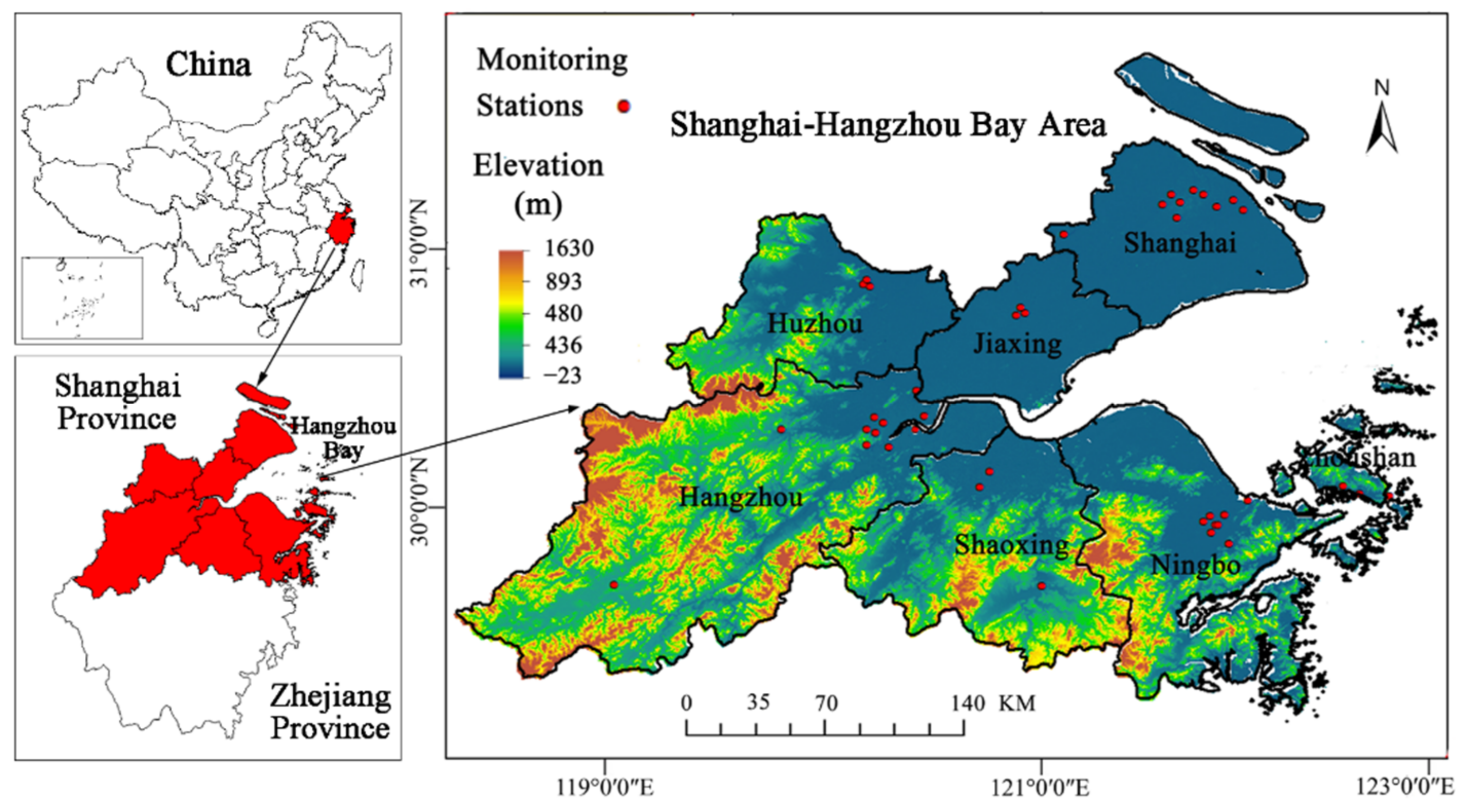
2.1. Study Area
2.2. Data Source
2.2.1. Vector and Elevation Data
2.2.2. Remote Sensing Data
2.2.3. Ground-Based AOD Observation Data
2.2.4. Ground-Level PM2.5 Observation Data
2.2.5. Population Density Data
2.3. Methods
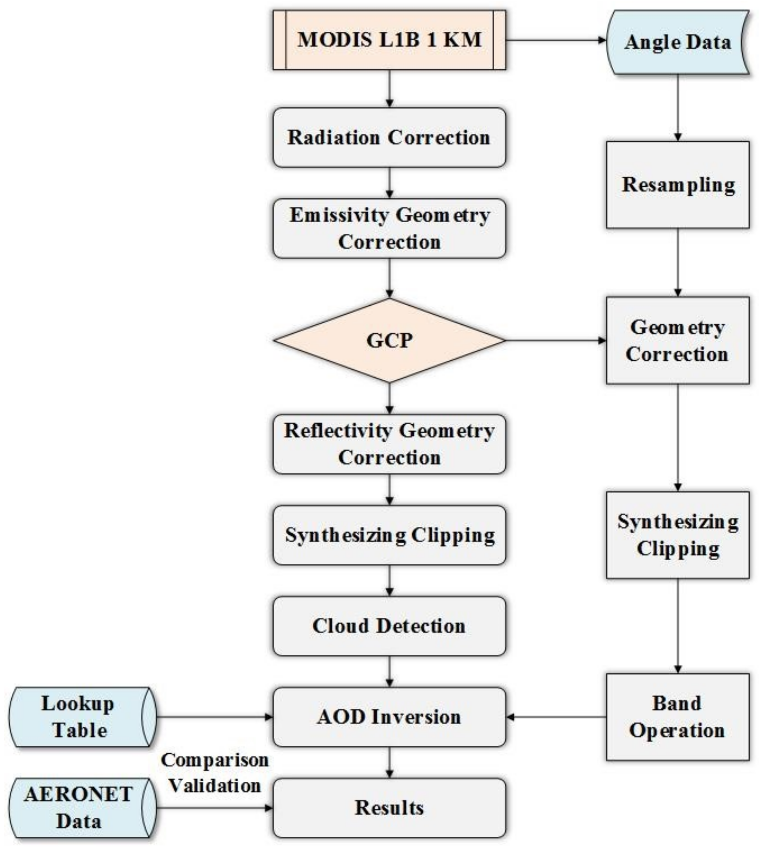
2.3.1. Enhanced Dark Target Algorithm (EDTA)
2.3.2. AOD-PM2.5 Spatial-Temporal Regression Models
2.3.3. Pearson’s and Spearman’s Rank Correlation Coefficients
2.3.4. Relative Exposure Risk Model
2.3.5. Spatial Autocorrelation Analysis
3. Results
3.1. AOD Inversion Results
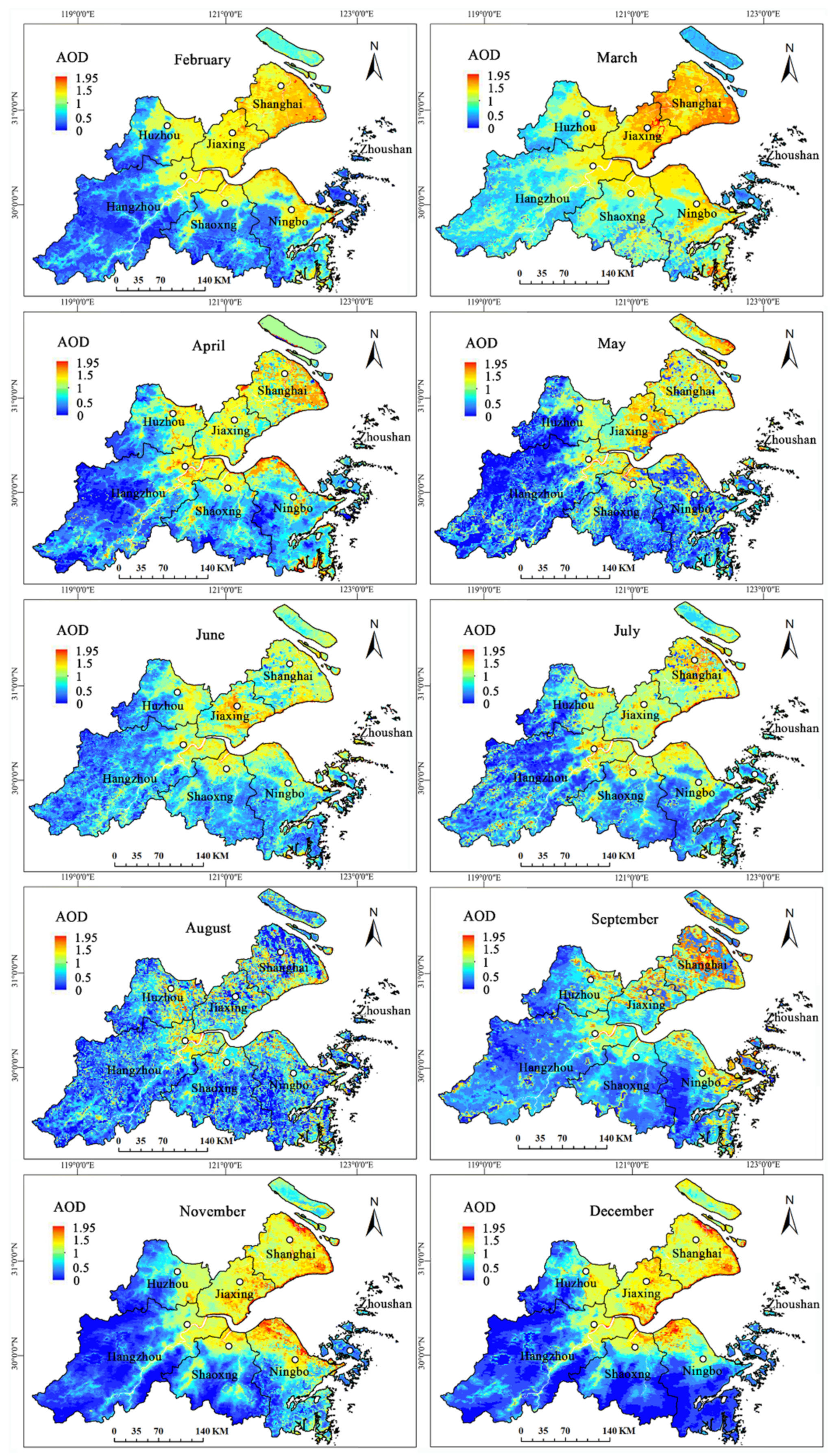
3.1.1. Monthly AOD Results
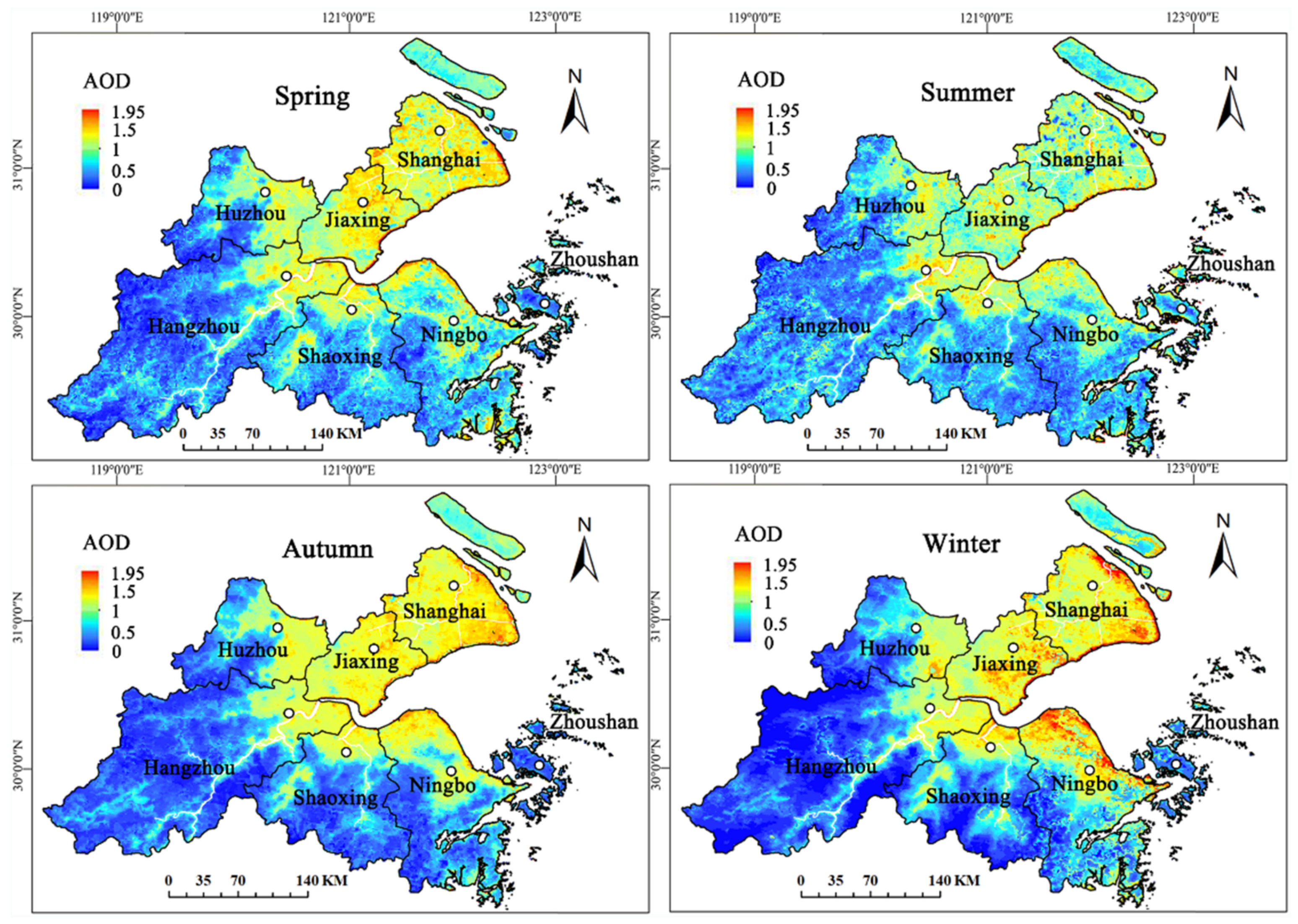
3.1.2. Seasonal AOD Results
3.1.3. Verification Result
3.2. Seasonal Spatial-Temporal Models
3.2.1. Correlation Analysis of Inversion AOD and Observation PM2.5
3.2.2. Seasonal Model Building and Verification
3.3. PM2.5 Estimation Results
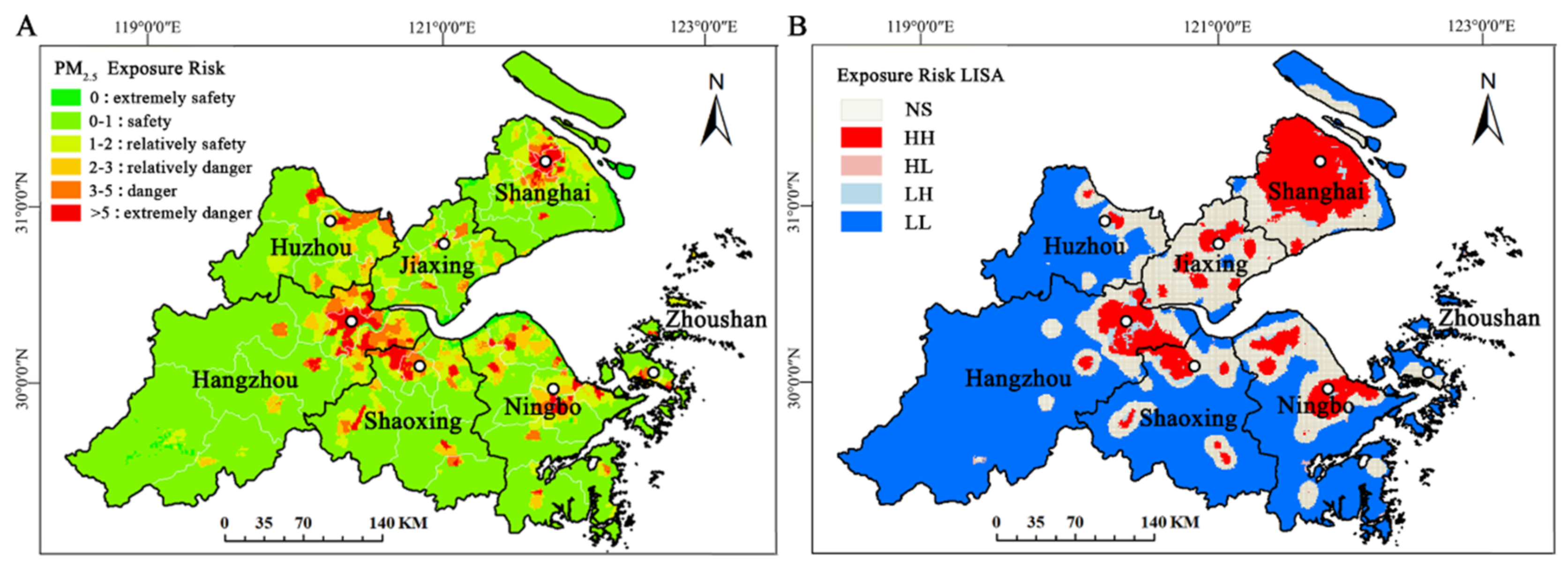
3.4. Exposure Risk Assessment
4. Discussion
5. Conclusions
Author Contributions
Funding
Institutional Review Board Statement
Informed Consent Statement
Data Availability Statement
Acknowledgments
Conflicts of Interest
Abbreviations
| GIS | Geographic Information Systems |
| RS | Remote sensing |
| SDGs | Sustainable Development Goals |
| PM2.5 | fine particulate matter (a diameter of less than 2.5 μm) |
| GOES | Geostationary Operational Environmental Satellite |
| METOP | European new generation weather operational satellites |
| PARASOL | Polarization and Anisotropy of Reflectances for Atmospheric Sciences coupled with Observations from a Lidar |
| MODIS | Moderate-resolution Imaging Spectror |
| AVHRR | Advanced Very High Resolution Radiometer |
| SeaWiFS | Sea-viewing Wide Field of View Sensor |
| POLDER | Polarization and Directionality of the Earth’s Reflectances |
| AOD | Aerosol Optical Depth |
| GEOS | Geosynchronous Earth Orbit Satellite |
| RAMS | Regional Atmospheric Modeling System |
| GLM | Generalized Linear Model |
| GAM | Generalized Additive Models |
| GWR | Geographically Weighted Regression |
| ML | Machine Learning |
| DTA | Dark Target Algorithm |
| EDTA | Enhanced Dark Target Algorithm |
| SHB | Shanghai-Hangzhou Bay |
| NSMS | National Standard Map Service platform in China |
| ESDC | Environmental Sciences and Data Center in China |
| NASA | National Aeronautics and Space Administration |
| LAADS | the Level-1 and Atmosphere Archive and Distribution System |
| AERONET | Aerosol Robotic Network |
| CEME | China Environmental Monitoring Center |
| LUT | Lookup Table |
| GCP | Ground Control Points |
| HDF | Hierarchical Data File |
References
- UN General Assembly. Transforming our World: The 2030 Agenda for Sustainable Development; United Nations: New York, NY, USA, 2015. [Google Scholar]
- Zhang, N.; Zhang, A.Q.; Wang, L.; Nie, P. Fine particulate matter and body weight status among older adults in China: Impacts and pathways. Health Place 2021, 69, 102571. [Google Scholar] [CrossRef] [PubMed]
- China Ministry of Ecological Environment. China’s Ecological Environment Status Report 2016 (Extract). Environ. Prot. 2017, 45, 35–47. [Google Scholar]
- China Ministry of Ecological Environment. China’s Ecological Environment Status Report 2017; China Ministry of Ecological Environment: Beijing, China, 2018. Available online: https://english.mee.gov.cn/Resources/Reports/soe/SOEE2017/201808/P020180801597738742758.pdf (accessed on 31 March 2022).
- China Ministry of Ecological Environment. China’s Ecological Environment Status Report 2018; China Ministry of Ecological Environment: Beijing, China, 2018. Available online: https://english.mee.gov.cn/Resources/Reports/soe/2018SOEE/202012/P020201215585208685493.pdf (accessed on 31 March 2022).
- China Ministry of Ecological Environment. China’s Ecological Environment Status Report 2019; China Ministry of Ecological Environment: Beijing, China, 2019. Available online: https://english.mee.gov.cn/Resources/Reports/soe/SOEE2019/202012/P020201215587453898053.pdf (accessed on 31 March 2022).
- China Ministry of Ecological Environment. China’s Ecological Environment Status Report 2020 (Extract); China Ministry of Ecological Environment: Beijing, China, 2021; pp. 47–68.
- Son, J.Y.; Lane, K.J.; Miranda, M.L.; Bell, M.L. Health disparities attributable to air pollutant exposure in North Carolina: Influence of residential environmental and social factors. Health Place 2020, 62, 102287. [Google Scholar] [CrossRef] [PubMed]
- Bates, J.T.; Weber, R.J.; Abrams, J.; Verma, V.; Fang, T.; Klein, M.; Stricklan, M.J.; Sarnat, S.E.; Chang, H.H.; Mulholland, J.A.; et al. Reactive oxygen species generation linked to sources of atmospheric particulate matter and cardiorespiratory effects. Environ. Sci. Technol. 2015, 49, 13605–13612. [Google Scholar] [CrossRef] [PubMed]
- Buteau, S.; Goldberg, M.S. A structured review of panel studies used to investigate associations between ambient air pollution and heart rate variability. Environ. Res. 2016, 148, 207–247. [Google Scholar] [CrossRef]
- Wang, C.C.; Tu, Y.F.; Yu, Z.L.; Lu, R.Z. PM2.5 and cardiovascular diseases in the elderly: An overview. Int. J. Environ. Res. Public Health 2015, 12, 8187–8197. [Google Scholar] [CrossRef] [Green Version]
- Chi, R.; Li, H.Y.; Wang, Q.; Zhai, Q.R.; Wang, D.D.; Wu, M.; Liu, Q.C.; Wu, S.W.; Ma, Q.B.; Deng, F.R.; et al. Association of emergency room visits for respiratory diseases with sources of ambient PM2.5. J. Environ. Sci. 2019, 86, 154–163. [Google Scholar] [CrossRef]
- Guan, W.J.; Zheng, X.Y.; Chung, K.F.; Zhong, N.S. Impact of air pollution on the burden of chronic respiratory diseases in China: Time for urgent action. Lancet 2016, 388, 1939–1951. [Google Scholar] [CrossRef]
- Gorai, A.; Tuluri, F.; Tchounwou, P. A GIS based approach for assessing the association between air pollution and asthma in New York State, USA. Int. J. Environ. Res. Public Health 2014, 11, 4845–4869. [Google Scholar] [CrossRef] [Green Version]
- Perera, F.P.; Tang, D.; Wang, S.; Vishnevetsky, J.; Zhang, B.Z.; Diaz, D.; Camann, D.; Rauh, V. Prenatal polycyclic aromatic hydrocarbon (PAH) exposure and child behavior at age 6–7 years. Environ. Health Perspect. 2012, 120, 921–926. [Google Scholar] [CrossRef] [Green Version]
- Zeng, Z.J.; Huo, X.; Wang, Q.H.; Wang, C.Y.; Hylkema, M.H.; Xu, X.J. PM2.5-bound PAHs exposure linked with low plasma insulin-like growth factor 1 levels and reduced child height. Environ. Int. 2020, 138, 105660. [Google Scholar] [CrossRef] [PubMed]
- Kim, C.; Jung, S.H.; Kang, D.R.; Kim, H.C.; Moon, K.T.; Hur, N.W.; Shin, D.C.; Suh, L. Ambient particulate matter as a risk factor for suicide. Am. J. Psychiatry 2010, 167, 1100–1107. [Google Scholar] [CrossRef] [PubMed]
- Sass, V.; Kravitz, W.N.; Karceski, S.M.; Hajat, A.; Crowder, K.; Takeuchi, D. The effects of air pollution on individual psychological distress. Health Place 2017, 48, 72–79. [Google Scholar] [CrossRef] [PubMed]
- Vert, C.; Sánchez-Benavides, G.; Martínez, D.; Gotsens, X.; Gramunt, N.; Cirach, M.; Molinuevo, J.L.; Sunyer, J.; Nieuwenhuijsen, M.J.; Crous-Bou, M.; et al. Effect of long-term exposure to air pollution on anxiety and depression in adults: A cross-sectional study. Int. J. Hyg. Environ. Health 2017, 220, 1074–1080. [Google Scholar] [CrossRef]
- Herbreteau, V.; Salem, G.; Souris, M.; Hugot, J.P.; Gonzalez, J.P. Thirty years of use and improvement of remote sensing, applied to epidemiology: From early promises to lasting frustration. Health Place 2007, 13, 400–403. [Google Scholar] [CrossRef]
- Maantay, J. Asthma and air pollution in the Bronx: Methodological and data considerations in using GIS for environmental justice and health research. Health Place 2007, 13, 32–56. [Google Scholar] [CrossRef]
- Golly, B.; Waked, A.; Weber, S.; Samake, A.; Jacob, V.; Conil, S.; Rangognio, J.; Chrétien, E.; Vagnot, M.P.; Robic, P.Y.; et al. Organic markers and OC source apportionment for seasonal variations of PM2.5 at 5 rural sites in France. Atmos. Environ. 2019, 198, 142–157. [Google Scholar] [CrossRef]
- Wang, Z.B.; Liang, L.W.; Wang, X.J. Spatio-temporal evolution patterns and influencing factors of PM2.5 in Chinese urban agglomerations. Acta Geogr. Sin. 2019, 12, 2614–2630. [Google Scholar]
- Shen, Y.; Yao, L. PM2.5, population exposure and economic effects in urban agglomerations of China using ground-based monitoring data. Int. J. Environ. Res. Public Health 2017, 14, 716. [Google Scholar] [CrossRef] [Green Version]
- Deuzé, J.L.; Bréon, F.M.; Devaux, C.; Goloub, P.; Herman, H.; Lafrance, B.; Maignan, F.; Marchand, A.; Nadal, F.; Perry, G.; et al. Remote sensing of aerosols over land surfaces from POLDER-ADEOS-1 polarized measurements. J. Geophys. Res. Atmos. 2001, 106, 4913–4926. [Google Scholar] [CrossRef] [Green Version]
- Kaufman, Y.J.; Tanré, D.; Remer, L.A.; Vermote, E.F.; Chu, A.; Holben, B.N. Operational remote sensing of tropospheric aerosol over land from EOS moderate resolution imaging spectroradiometer. J. Geophys. Res. Atmos. 1997, 102, 17051–17067. [Google Scholar] [CrossRef]
- Lyons, W.A.; Husar, R.B. SMS/GOES visible images detect a synoptic-scale air pollution episode. Mon. Weather Rev. 1976, 104, 1623–1626. [Google Scholar] [CrossRef] [Green Version]
- Li, C.C.; Mao, J.T.; Liu, Q.H.; Yuan, Z.B.; Wang, M.H.; Liu, X.Y. Remote sensing aerosol with MODIS and the application of MODIS aerosol products. Sci. China Ser. D 2005, 35, 177–186. [Google Scholar]
- Wang, Z.T.; Chen, L.F.; Zhang, Y.; Han, D. Urban surface aerosol monitoring using DDV method from MODIS Data. Remote Sens. Technol. Appl. 2008, 23, 284–288. [Google Scholar]
- Kaufman, Y.J.; Sendra, C. Algorithm for automatic atmospheric corrections to visible and near-IR satellite imagery. Int. J. Remote Sens. 1988, 9, 1357–1381. [Google Scholar] [CrossRef]
- Levy, R.C.; Remer, L.A.; Mattoo, S.; Vermote, E.F.; Kaufman, Y.J. Second-generation operational algorithm: Retrieval of aerosol properties over land from inversion of Moderate Resolution Imaging Spectroradiometer spectral reflectance. J. Geophys. Res. Atmos. 2007, 112, D13211. [Google Scholar] [CrossRef] [Green Version]
- Holben, B.N.; Vermote, E.; Kaufman, Y.J.; Tanré, D.; Kalb, V. Aerosol retrieval over land from AVHRR data-application for atmospheric correction. IEEE Trans. Geosci. Remote Sens. 1992, 30, 212–222. [Google Scholar] [CrossRef]
- Tanré, D.; Devaux, C.; Herman, M.; Santer, R.; Gac, J.Y. Radiative properties of desert aerosols by optical ground-based measurements at solar wavelengths. J. Geophys. Res. Atmos. 1988, 93, 14223–14231. [Google Scholar] [CrossRef]
- Hsu, N.C.; Tsay, S.C.; King, M.D.; Herman, J.R. Aerosol properties over bright-reflecting source regions. IEEE Trans. Geosci. Remote Sens. 2004, 42, 557–569. [Google Scholar] [CrossRef]
- Hsu, N.C.; Tsay, S.C.; King, M.D.; Herman, J.R. Deep blue retrievals of Asian aerosol properties during ACE-Asia. IEEE Trans. Geosci. Remote Sens. 2006, 44, 3180–3195. [Google Scholar] [CrossRef]
- Lyapustin, A.; Martonchik, J.; Wang, Y.J.; Laszlo, I.; Korkin, S. Multiangle implementation of atmospheric correction (MAIAC): 1. Radiative transfer basis and look-up tables. J. Geophys. Res. Atmos. 2011, 116, D03210. [Google Scholar] [CrossRef]
- Lyapustin, A.; Wang, Y.; Laszlo, I.; Kahn, R.; Korkin, S.; Remer, L.; Levy, R.; Reid, J.S. Multiangle implementation of atmospheric correction (MAIAC): 2. Aerosol algorithm. J. Geophys. Res. Atmos. 2011, 116, D03211. [Google Scholar] [CrossRef]
- Guo, J.; Xia, F.; Zhang, Y.; Liu, H.; Li, J.; Lou, M.; He, J.; Yan, Y.; Wang, F.; Min, M.; et al. Impact of diurnal variability and meteorological factors on the PM2.5-AOD relationship: Implications for PM2.5 remote sensing. Environ. Pollut. 2017, 221, 94–104. [Google Scholar] [CrossRef] [PubMed] [Green Version]
- Kumar, N. What can affect AOD-PM2.5 association? Environ. Health Perspect. 2010, 118, 109–110. [Google Scholar] [CrossRef] [PubMed] [Green Version]
- Li, J.; Carlson, B.E.; Lacis, A.A. How well do satellite AOD observations represent the spatial and temporal variability of PM2.5 concentration for the United States? Atmos. Environ. 2015, 102, 260–273. [Google Scholar]
- Donkelaar, A.V.; Martin, R.; Brauer, M.; Kahn, R.; Levy, R.; Verduzco, C.; Villeneuve, P.J. Global estimates of ambient fine particulate matter concentrations from satellite-based aerosol optical depth: Development and application. Environ. Health Perspect. 2010, 118, 847–855. [Google Scholar] [CrossRef] [Green Version]
- Donkelaar, A.V.; Martin, R.V.; Park, R.J. Estimating ground-level PM2.5 with aerosol optical depth determined from satellite remote sensing. J. Geophys. Res. Atmos. 2006, 111, D21201. [Google Scholar] [CrossRef]
- Liu, Y.; Park, R.J.; Jacob, D.J.; Li, Q.B.; Kilaru, V.; Sarnat, J.A. Mapping annual mean ground-level PM2.5 concentrations using multiangle imaging spectroradiometer aerosol optical thickness over the contiguous United States. J. Geophys. Res. Atmos. 2004, 109, D22. [Google Scholar] [CrossRef]
- Tao, J.H.; Zhang, M.G.; Chen, L.F.; Wang, Z.F.; Su, L.; Ge, C.; Xiao, H.; Zou, M.M. A method to estimate concentrations of surface-level particulate matter using satellite-based aerosol optical thickness. Sci. China Ser. D 2013, 8, 1422–1433. [Google Scholar] [CrossRef]
- Chen, L.F.; Tao, J.H.; Wang, Z.F.; Li, S.S.; Zhang, Y.; Fan, M.; Li, X.Y.; Yu, C.; Zou, M.M.; Su, L.; et al. Review of satellite remote sensing of air quality. J. Atmos. Environ. Opt. 2015, 10, 117–125. [Google Scholar]
- Wang, Z.F.; Chen, L.F.; Tao, J.H.; Zhang, Y.; Su, B. Satellite-based estimation of regional particulate matter (PM) in Beijing using vertical-and-RH correcting method. Remote Sens. Environ. 2010, 114, 50–63. [Google Scholar] [CrossRef]
- Li, C.C.; Mao, J.T.; Lau, A.K.H.; Yuan, Z.B.; Wang, M.H.; Liu, X.Y. Application of MODIS satellite products to the air pollution research in Beijing. Sci. China Ser. D 2005, 48, 209–219. [Google Scholar]
- Chu, D.A.; Tsai, T.C.; Chen, J.P.; Chang, S.C.; Jeng, Y.J.; Chiang, W.L.; Lin, N.H. Interpreting aerosol lidar profiles to better estimate surface PM2.5 for columnar AOD measurements. Atmos. Environ. 2013, 79, 172–187. [Google Scholar] [CrossRef]
- Hutchison, K.D.; Faruqui, S.J.; Smith, S. Improving correlations between MODIS aerosol optical thickness and ground-based PM2.5 observations through 3D spatial analyses. Atmos. Environ. 2008, 42, 530–543. [Google Scholar] [CrossRef]
- Liu, Y.; Sarnat, J.A.; Kilaru, V.K.; Jacob, D.J.; Koutrakis, P. Estimating ground-level PM2.5 in the eastern United States using satellite remote sensing. Environ. Sci. Technol. 2005, 39, 3269–3278. [Google Scholar] [CrossRef] [Green Version]
- Liu, Y.; Paciorek, C.J.; Koutrakis, P. Estimating regional spatial and temporal variability of PM2.5 concentrations using satellite data, meteorology, and land use information. Environ. Health Perspect. 2009, 117, 886–892. [Google Scholar] [CrossRef] [Green Version]
- Strawa, A.W.; Chatfield, R.B.; Legg, M.; Scarnato, B.; Esswein, R. Improving retrievals of regional fine particulate matter concentrations from Moderate Resolution Imaging Spectroradiometer (MODIS) and Ozone Monitoring Instrument (OMI) multisatellite observations. J. Air Waste Manag. Assoc. 2013, 63, 1434–1446. [Google Scholar] [CrossRef]
- Hu, X.F.; Waller, L.A.; AI-Hamdan, M.Z.; Crosson, W.L.; Estes, M.G., Jr.; Estes, S.M.; Quattrochi, D.A.; Sarnat, J.A.; Liu, Y. Estimating ground-level PM2.5 concentrations in the southeastern U.S. using geographically weighted regression. Environ. Res. 2013, 121, 1–21. [Google Scholar] [CrossRef]
- Zhang, L.L.; Pan, J.H.; Lai, J.B.; Wei, S.M.; Wang, Y.; Zhang, D.H. Estimation of PM2.5 mass concentrations in Beijing-Tianjin-Hebei region based on geographically weighted regression and spatial downscaling method. Acta Sci. Circum. 2019, 39, 832–842. [Google Scholar] [CrossRef]
- Chen, H.; Li, Q.; Zhang, Y.H.; Zhou, C.Y.; Wang, Z.T. Estimations of PM2.5 concentrations based on the method of geographically weighted regression. Acta Sci. Circum. 2016, 36, 2142–2151. [Google Scholar]
- Deng, Y.; Liu, J.P.; Liu, Y.; Xu, S.H. Spatial distribution estimation of PM2.5 concentration in Beijing by applying Bayesian geographic weighted regression model. Sci. Surv. Mapp. 2018, 43, 39–45. [Google Scholar]
- Zhai, L.; Li, S.; Zou, B.; Sang, H.Y.; Fang, X.; Xu, S. An improved geographically weighted regression model for PM2.5 concentration estimation in large areas. Atmos. Environ. 2018, 181, 145–154. [Google Scholar] [CrossRef]
- Wei, J.; Huang, W.; Li, Z.Q.; Xue, W.H.; Peng, Y.R.; Sun, L. Estimating 1-km-resolution PM2.5 concentrations across China using the space-time random forest approach. Remote Sens. Environ. 2019, 231, 111221. [Google Scholar] [CrossRef]
- Xue, T.; Zheng, Y.; Tong, D.; Zheng, B.; Li, X.; Zhu, T. Spatiotemporal continuous estimates of PM2.5 concentrations in China, 2000-2016: A machine learning method with inputs from satellites, chemical transport model, and ground observations. Environ Int. 2019, 123, 345–357. [Google Scholar] [CrossRef]
- Wang, Z.F.; Zeng, Q.L.; Chen, L.F.; Tao, J.H.; Fan, M.; Zhang, Z.Y. Research progress of methodology and applications of PM2.5 estimation using satellite remote sensing. Environ. Monit. Forew. 2019, 11, 33–38. [Google Scholar]
- Zou, B.; Peng, F.; Jiao, L.M.; Weng, M. GIS aided spatial zoning of high-resolution population exposure to air pollution. Geomat. Inform. Sci. Wuhan Univ. 2013, 38, 334–338. [Google Scholar]
- Tong, L.G.; Li, X.M.; Huang, Z.; Zhang, J.; Tian, S.Z. Study on risk of population exposure to PM2.5 in Baotou City. J. Arid Land Resour. Environ. 2017, 31, 50–54. [Google Scholar]
- Lu, M.; Schmitz, O.; Vaartjes, I.; Karssenberg, D. Activity-based air pollution exposure assessment: Differences between homemakers and cycling commuters. Health Place 2019, 60, 102233. [Google Scholar] [CrossRef]
- Park, Y.M. Assessing personal exposure to traffic-related air pollution using individual travel-activity diary data and an on-road source air dispersion model. Health Place 2020, 63, 102351. [Google Scholar] [CrossRef]
- Li, C.C.; Mao, J.T.; Liu, Q.H.; Chen, J.Z.; Yuan, Z.B.; Liu, X.Y.; Zhu, A.H.; Liu, G.Q. Distribution and seasonal variation of aerosol optical depth using MODIS data, eastern China. Chin. Sci. Bull. 2003, 48, 2094–2100. [Google Scholar]
- Wang, L.L.; Xin, J.Y.; Wang, Y.S.; Li, Z.Q.; Wang, P.C.; Liu, G.R. Evaluation on the applicability of MODIS aerosol products in China from CSHNET. Chin. Sci. Bull. 2007, 52, 477–486. [Google Scholar]
- Holben, B.N.; Eck, T.F.; Slutsker, I.; Tanré, D.; Buis, J.P.; Setzer, A.; Vermote, E.; Reagan, J.A.; Kaufman, Y.J.; Nakajima, T.; et al. AERONET: A federated instrument network and data archive for aerosol characterization. Remote Sens. Environ. 1998, 66, 1–16. [Google Scholar] [CrossRef]
- Tatem, A.J. WorldPop, open data for spatial demography. Sci. Data 2017, 4, 170004. [Google Scholar] [CrossRef] [PubMed]
- Kaufman, Y.J.; Wald, A.E.; Remer, L.A.; Gao, B.C.; Li, R.R.; Flynn, L. The MODIS 2.1µm channel-correlation with visible reflectance for use in remote sensing of aerosol. IEEE Trans. Geosci. Remote Sens. 1997, 35, 1286–1298. [Google Scholar] [CrossRef]
- Zhao, Z.Q.; Li, A.N.; Bian, J.H.; Huang, C.Q. An improved DDV method to retrieve AOT for HJ CCD image in typical mountainous areas. Spectrosc. Spect. Anal. 2015, 35, 1479–1487. [Google Scholar]
- Ångström, A. The parameter of atmospheric turbidity. Tellus 1964, 16, 64–75. [Google Scholar] [CrossRef] [Green Version]
- Kousa, A.; Oglesby, L.; Koistinen, K.; Künzli, N.; Jantunen, M. Exposure chain of urban air PM2.5: Associations between ambient fixed site, residential outdoor, indoor, workplace and personal exposures in four European cities in the EXPOLIS-study. Atmos. Environ. 2002, 36, 3031–3039. [Google Scholar] [CrossRef]
- Zhang, L.L.; Pan, J.H. Spatial-temporal pattern of population exposure risk to PM2.5 in China. China Environ. Sci. 2020, 40, 7427. [Google Scholar]
- Zhang, X.Y.; Hu, H.B. Risk assessment of exposure to PM2.5 in Beijing using multi-source data. Acta Sci. Nat. Univ. Peking 2018, 54, 1103–1113. [Google Scholar]


| City | Site | Longitude (°E) | Latitude (°N) | Data |
|---|---|---|---|---|
| Shanghai | SONET_Shanghai | 121.481 | 31.284 | Level 1.0 a, Level 1.5 b |
| Shanghai_Minhang | 121.397 | 31.130 | null | |
| Shanghai_Met | 121.549 | 31.221 | null | |
| Hangzhou | LA-TM | 119.440 | 30.324 | null |
| Hangzhou-ZFU | 119.727 | 30.257 | null | |
| Hangzhou_City | 120.157 | 30.290 | null | |
| Qiandaohu | 119.053 | 29.556 | null | |
| Ningbo | Ningbo | 121.547 | 29.860 | null |
| Zhoushan | SONET_Zhoushan | 122.188 | 29.994 | Level 1.0 a, Level 1.5 b |
| City | Monitoring Station | Longitude (°E) | Latitude (°N) |
|---|---|---|---|
| Shanghai | Putuo | 121.3984 | 31.2637 |
| NO.15 Factory | 121.3614 | 31.2228 | |
| Hongkou | 121.4919 | 31.2825 | |
| Shanghai Normal University | 121.4232 | 31.1675 | |
| Sipiao | 121.5360 | 31.2659 | |
| Dianshan Lake | 120.9382 | 31.0927 | |
| Jingan | 121.4363 | 31.2305 | |
| Chuansha | 121.7042 | 31.1994 | |
| Pudong New Area | 121.6634 | 31.2428 | |
| Zhangjiang | 121.5918 | 31.2108 | |
| Jiaxing | Qinghe Primary School | 120.7543 | 30.7819 |
| Jiaxing College | 120.7372 | 30.7517 | |
| Disabled Persons’ Federation | 120.7739 | 30.7601 | |
| Hangzhou | Binjiang | 120.1924 | 30.1876 |
| Xixi | 120.1000 | 30.2645 | |
| Qiandao Lake | 119.0214 | 29.6020 | |
| Xiasha | 120.3442 | 30.3221 | |
| Wolong Bridge | 120.1385 | 30.2493 | |
| Zhejiang Agricultural University | 119.7355 | 30.2621 | |
| Zhaohui NO.5 Community | 120.1688 | 30.2940 | |
| Hemu Primary School | 120.1312 | 30.3161 | |
| Linping | 120.3133 | 30.4272 | |
| Chengxiang | 120.3052 | 30.2615 | |
| Yunqi | 120.1010 | 30.1989 | |
| Shaoxing | Paojiang | 120.6238 | 30.0842 |
| East Management Committee of Development Zone | 120.8460 | 29.5986 | |
| Shuxia Wang | 120.5828 | 30.0159 | |
| Ningbo | Environmental Protection Building | 121.5865 | 29.8582 |
| Wanli College | 121.5695 | 29.8230 | |
| Longsai Hospital | 121.7223 | 29.9596 | |
| Sanjiang Middle School | 121.5647 | 29.8940 | |
| Qiangtang Waterwork | 121.6440 | 29.7770 | |
| Taigu Primary School | 121.5985 | 29.8596 | |
| Environmental Monitoring Center | 121.5351 | 29.8709 | |
| Wanli International School | 121.6234 | 29.9019 | |
| Zhoushan | Dinghai TanFeng | 122.1320 | 30.0240 |
| Putuo Donggang | 122.3285 | 29.9791 | |
| Lincheng New Area | 122.2020 | 29.9885 | |
| Huzhou | Renhuangshan New Area | 120.0976 | 30.9000 |
| West Waterwork | 120.0844 | 30.8811 | |
| Wuxing | 120.1158 | 30.8710 |
| Major Parameters | Settings |
|---|---|
| Satellite zenith angle | 0°, 12°, 24°, 36°, 48°, 60° |
| Solar zenith angle | 0°, 12°, 24°, 36°, 48°, 60° |
| Relative azimuth angle | 0~180°, 24° (interval) |
| AOD at 550 nm wavelength | 0, 0.25, 0.50, 1.00, 1.50, 1.95 |
| Central wavelength | 470 nm, 660 nm, 2100 nm |
| Elevation | 0 |
| Surface type | Vegetation |
| Regression Model | Equation |
|---|---|
| Linear | y = a0 + a1x |
| Logarithmic | y = a0 + a1ln(x) |
| Exponential | y = a0 × ea1x |
| Power | y = a0(xa1) |
| Quadratic Polynomial | y = a0 + a1x + a2x2 |
| Cubic Polynomial | y = a0 + a1x + a2x2 + a3x3 |
| Site | Days | Date | AOD Value | |
|---|---|---|---|---|
| Inversion | Observation | |||
| SONET_Shanghai | 10 | 1 May 2016 | 0.610 | 0.785 |
| 3 May 2016 | 0.792 | 0.890 | ||
| 4 May 2016 | 0.500 | 0.449 | ||
| 12 May 2016 | 0.375 | 0.304 | ||
| 15 May 2016 | 0.400 | 0.551 | ||
| 16 May 2016 | 0.917 | 0.346 | ||
| 17 May 2016 | 0.400 | 0.222 | ||
| 24 May 2016 | 1.170 | 1.194 | ||
| 25 May 2016 | 1.246 | 0.951 | ||
| 6 June 2016 | 0.720 | 1.153 | ||
| SONET_Zhoushan | 11 | 30 April 2016 | 0.808 | 0.464 |
| 1 May 2016 | 0.730 | 0.474 | ||
| 3 May 2016 | 0.320 | 0.314 | ||
| 4 May 2016 | 0.700 | 0.775 | ||
| 11 May 2016 | 1.170 | 0.815 | ||
| 12 May 2016 | 0.563 | 0.534 | ||
| 16 May 2016 | 0.200 | 0.218 | ||
| 17 May 2016 | 0.150 | 0.154 | ||
| 18 May 2016 | 0.200 | 0.199 | ||
| 24 May 2016 | 1.000 | 1.022 | ||
| 6 June 2016 | 0.350 | 0.360 | ||
| M a | 0.634 | 0.580 | ||
| SD b | 0.334 | 0.328 | ||
| R c | 0.781 | 0.781 | ||
| Significant (bilateral) | 0 | 0 | ||
| Month | Sample | N b | Season | Sample | N b | ||
|---|---|---|---|---|---|---|---|
| March | AOD | 0.021 | 41 | Spring | 0.538 | 123 | |
| PM2.5 | |||||||
| April | AOD | 0.406 | 41 | AOD | |||
| PM2.5 | PM2.5 | ||||||
| May | AOD | 0.631 | 41 | ||||
| PM2.5 | |||||||
| June | AOD | 0.443 | 41 | Summer | 0.684 | 123 | |
| PM2.5 | |||||||
| July | AOD | 0.432 | 41 | AOD | |||
| PM2.5 | PM2.5 | ||||||
| August | AOD | 0.607 | 41 | ||||
| PM2.5 | |||||||
| September | AOD | 0.395 | 41 | Autumn | 0.474 | 82 | |
| PM2.5 | AOD | ||||||
| November | AOD | 0.138 | 41 | PM2.5 | |||
| PM2.5 | |||||||
| December | AOD | 0.314 | 41 | Winter | 0.341 | 82 | |
| PM2.5 | AOD | ||||||
| February | AOD | 0.121 | 41 | PM2.5 | |||
| PM2.5 |
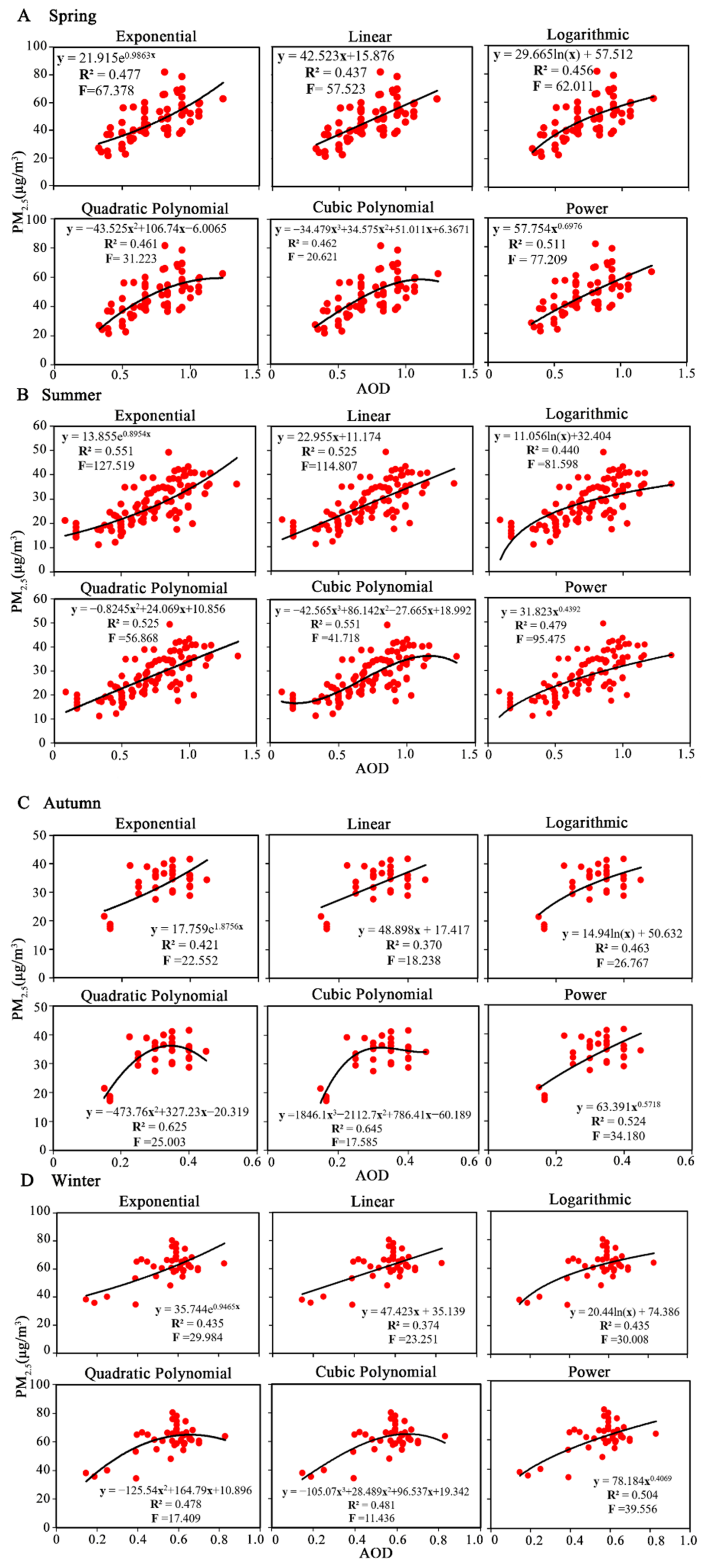
| Season | Model | Equation | Model Building | Model Verification | ||
|---|---|---|---|---|---|---|
| R2 | F | R2 | RMSE | |||
| Spring | A a | y = 42.523x + 15.876 | 0.437 | 57.523 | 0.514 | 6.587 |
| B b | y = 29.665ln(x) + 57.512 | 0.456 | 62.011 | 0.503 | 6.719 | |
| C c | y = 21.915e0.9863x | 0.477 | 67.378 | 0.504 | 6.246 | |
| D d | y = −43.525x2 + 106.74x − 6.0065 | 0.461 | 31.223 | 0.506 | 6.829 | |
| E e | y = −34.479x3 + 34.575x2 + 51.011x + 6.3671 | 0.462 | 20.621 | 0.515 | 6.900 | |
| F f | y = 57.754x0.6976 | 0.511 | 77.209 | 0.513 | 6.204 | |
| Summer | A a | y = 22.955x + 11.174 | 0.525 | 114.807 | 0.590 | 4.432 |
| B b | y = 11.056ln(x) + 32.404 | 0.440 | 81.598 | 0.418 | 5.254 | |
| C c | y = 13.855e0.8954x | 0.551 | 127.519 | 0.640 | 3.979 | |
| D d | y = −0.8245x2 + 24.069x + 10.856 | 0.525 | 56.868 | 0.588 | 4.440 | |
| E e | y = −42.565x3 + 86.142x2 − 27.665x + 18.992 | 0.551 | 41.718 | 0.606 | 4.113 | |
| F f | y = 31.823x0.4392 | 0.479 | 95.457 | 0.518 | 4.313 | |
| Autumn | A a | y = 48.898x + 17.417 | 0.370 | 18.238 | 0.488 | 8.857 |
| B b | y = 14.94ln(x) + 50.632 | 0.463 | 26.767 | 0.515 | 7.534 | |
| C c | y = 17.759e1.8756x | 0.421 | 22.552 | 0.478 | 8.980 | |
| D d | y = −473.76x2 + 327.23x − 20.319 | 0.625 | 25.003 | 0.455 | 9.010 | |
| E e | y = 1846.1x3 − 2112.7x2 + 786.41x − 60.189 | 0.645 | 17.585 | 0.497 | 9.087 | |
| F f | y = 63.391x0.5718 | 0.524 | 34.180 | 0.520 | 7.893 | |
| Winter | A a | y = 47.423x + 35.139 | 0.373 | 23.251 | 0.508 | 7.957 |
| B b | y = 20.44ln(x) + 74.386 | 0.435 | 30.008 | 0.547 | 7.621 | |
| C c | y = 35.744e0.9465x | 0.435 | 29.984 | 0.471 | 7.706 | |
| D d | y = −125.54x2 + 164.79x + 10.896 | 0.478 | 17.409 | 0.550 | 7.450 | |
| E e | y = −105.07x3 + 28.489x2 + 96.537x + 19.342 | 0.481 | 11.436 | 0.553 | 7.429 | |
| F f | y = 78.184x0.4069 | 0.504 | 39.556 | 0.540 | 7.392 | |
Publisher’s Note: MDPI stays neutral with regard to jurisdictional claims in published maps and institutional affiliations. |
© 2022 by the authors. Licensee MDPI, Basel, Switzerland. This article is an open access article distributed under the terms and conditions of the Creative Commons Attribution (CC BY) license (https://creativecommons.org/licenses/by/4.0/).
Share and Cite
Xu, D.; Lin, W.; Gao, J.; Jiang, Y.; Li, L.; Gao, F. PM2.5 Exposure and Health Risk Assessment Using Remote Sensing Data and GIS. Int. J. Environ. Res. Public Health 2022, 19, 6154. https://0-doi-org.brum.beds.ac.uk/10.3390/ijerph19106154
Xu D, Lin W, Gao J, Jiang Y, Li L, Gao F. PM2.5 Exposure and Health Risk Assessment Using Remote Sensing Data and GIS. International Journal of Environmental Research and Public Health. 2022; 19(10):6154. https://0-doi-org.brum.beds.ac.uk/10.3390/ijerph19106154
Chicago/Turabian StyleXu, Dan, Wenpeng Lin, Jun Gao, Yue Jiang, Lubing Li, and Fei Gao. 2022. "PM2.5 Exposure and Health Risk Assessment Using Remote Sensing Data and GIS" International Journal of Environmental Research and Public Health 19, no. 10: 6154. https://0-doi-org.brum.beds.ac.uk/10.3390/ijerph19106154