System Reliability Assessment Based on Energy Dissipation: Modeling and Application in Electro-Hydrostatic Actuation System

1
School of Automation Science and Electrical Engineering, Beihang University, Beijing 100191, China
2
Energy Department, Politecnico di Milano, Via La Masa 34, 20156 Milano, Italy
*
Author to whom correspondence should be addressed.
Energies 2019, 12(18), 3572; https://0-doi-org.brum.beds.ac.uk/10.3390/en12183572
Submission received: 2 August 2019
/
Revised: 29 August 2019
/
Accepted: 16 September 2019
/
Published: 18 September 2019
Abstract
:This paper addresses a new reliability model, based on energy dissipation, considering performance degradation behaviors. Different from the two-state reliability model and traditional reliability model based on failure rate statistics, this paper focuses on the component energy loss due to its fault evolution, such as fatigue, aging and wear, and presents a reliability model based on the component’s energy dissipation, as well as establishing a power dissipation constrained reliability model for degradation-based reliability assessment. As a demonstration, the proposed method is applied to model and evaluate the failure behavior of the electro-hydrostatic actuation system. The results indicate that the proposed method is effective in describing its life-cycle degradation in the energy field, and provides a reliability assessment based on energy dissipation.
1. Introduction
Physical degradation inevitably occurs in engineering systems, which leads to potential risks and hazards. Traditional binary-state reliability models assume that the system is either running perfectly or has completely failed, and is therefore unable to reveal real situations. Multi-state models provide a more realistic depiction, by introducing a finite number of states. Many studies describe the multiple states of the system degradation process and estimate the system reliability based on multi-state models, including the universal generating function technique [1,2], the structure function approach [3], the stochastic process approach [4,5], and the Monte-Carlo simulation technique [6]. The physics-of-failure (PoF) models provide comprehensive interpretation of statistical data based on physics and mechanistic methods. The models serve as good alternatives when the reliable data are limited, by modeling failure mechanisms such as fatigue, aging and wear. In 2002, the PoF-based methods were selected by the IEEE for system reliability prediction [7]. Recently, increasing attention has been given to PoF-based reliability modeling methods. Sun et al. [8] analyzed the reliability of the electrolytic capacitor in light-emitting diode drivers using PoF-based methods. Ma et al. [9] assessed the reliability of a power electronics system by establishing PoF models of components. Zeng et al. [10] studied the effect of component dependency on system reliability by considering failure collaboration using PoF models. The PoF approaches employ well-developed knowledge and there is no common method to build a PoF model. When information limitation is considered, probabilistic physics-of-failure (PPoF) methods [11] are proposed to address the related uncertainties.
For a system containing multiple components, system reliability should concern the relationship between various components. To identify the key components that mostly influence the safety and reliability of a system is difficult in practice. Based on different physical arrangements of components, the reliability block diagram, event tree analysis and fault tree analysis [12] are frequently used to model the statistical effect of components on the entire system. Owing to the dynamic characteristics of systems, dynamic reliability block diagrams [13], dynamic fault trees [14] and colored petri nets [15], combined with Markov chains and Monte-Carlo methods, are proposed [16,17]. Since the degrading behavior of a component may have an influence on another component, copulas functions are employed to describe the dependency of the two-degradation process [18,19]. Typically, by using such methods, the failure of components is defined individually by a certain threshold. For example, a pump is believed to be failed when the leakage flow reaches a threshold. Practically, with respect to a whole system, it is hard to define an exact failure threshold for each component under different work conditions. For example, the leakage flow of the pump reaches the failure threshold of itself, but the system can still provide enough flow for external loads. The system reliability evaluation based on individual failure threshold may not be a proper method.
To achieve the unified evaluation of a system with diverse components, there are practical difficulties that make it hard to normalize the effect of a single component by different failure mechanisms on the whole system. The systems in the engineering field, in terms of their basic functions, can be divided into a signal transfer system, an energy transfer system, and a mass transfer system. Due to the similar transmission characteristics derived from conservation law, a mass transfer system can be regarded as a special type of energy transfer system. Given input energy, the reliability of an energy transfer system is defined as the probability of providing enough output energy under stated conditions, for a specific period of time. In this paper, we focus on the energy loss during the energy transferring process of energy transfer systems. Energy works as the currency, evaluating performance degradation by different mechanisms of components with different types of energy. A unified indicator of performance degradation, named failure related energy dissipation, is proposed, which can be obtained from PPoF models. Generally, the Markov process assumes that the states transfer time interval is very small and negligible, while the performance degradation of a component is related to time in real application. Considering the state transfer time interval and the different degradation rate between states in the actual degradation process of components, the semi-Markov process [20,21] is an effective to way to model the failure behavior and degradation states relationship, which is employed to build the system reliability model. The system reliability is, then, evaluated globally, combining the multi-state model of the system with the PPoF models of the components.
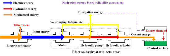
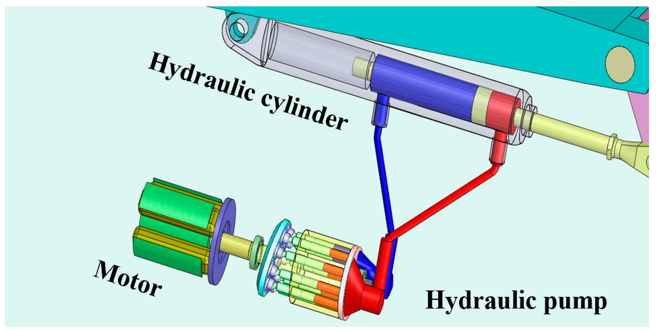
In more electrical aircraft, an electro-hydrostatic actuation system (EHA) replaces some hydraulic actuation systems in the auxiliary surface control system, with convenient electrical transmission and local hydraulic power supply. In EHA, the motor adopts electrical energy and converts it into mechanical energy through electromagnetic energy. The hydraulic pump is driven by the motor to transmit the mechanical energy through hydraulic power. The cylinder accepts the high-pressure oil and drives the piston elongation and contraction. Since the performance of EHA degrades with operational time, its failure process can be regarded as a combination of multiple degenerated levels of motor, hydraulic pump and cylinder. EHA is a typical energy transfer system and taken as an example to illustrate the proposed system-level reliability assessment method.
The rest of the paper is organized as follows: in Section 2, the energy dissipation is firstly defined, and a multi-state reliability model is established based on energy dissipation. In Section 3, an illustrative method is proposed showing the parameter estimation process by a PPoF model with Gaussian uncertainties. In Section 4, the proposed method is conducted in EHA. The PPoF models of hydraulic pump, motor and hydraulic cylinder are established to obtain the failure related energy dissipation and the reliability assessment results are discussed. In Section 5, some conclusions and remarks are presented.
2. Reliability Model Based on Energy Dissipation
In this paper, we focus on a type of energy transfer system that involves multiple types of energy, such as hydraulic, mechanical and electrical energy. Different types of energy are transferred, stored and transformed by energy transfer components for different desired effects. During the process, degrading behavior such as wear, fatigue and aging inevitably occurs, which results in thermal and volumetric energy loss. Failure-related energy dissipation is introduced to measure the failure behavior of energy transfer system components and characterizes the reliability based on energy dissipation.
2.1. Failure Related Energy Dissipation (FED)
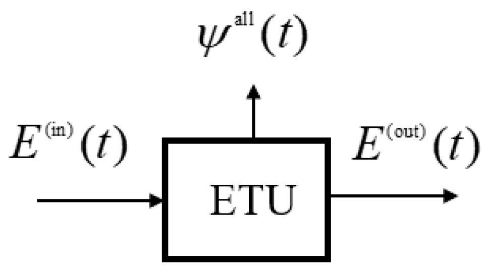
A practical energy transfer system normally contains diversiform energy transfer components, including electrical components, mechanical components, hydraulic components and pneumatic components. Although different components suffer from different types of performance degradation, the similarity is that each of these components transmit energy to implement different functions. For a unified description of the physical degrading process, such components are defined as the energy transmission unit (ETU) in this paper. Assuming that is the input energy of ETU from an upstream component, is the output energy to the downstream component and is the total energy dissipation of ETU that will lead to fault development. A general model of ETU is shown in Figure 1.
Considering single failure mode, three typical examples of physical degradation are taken to show how to use energy dissipation to describe the failure behavior of ETU.
(a) Wear and tear
According to wear theory [22], the wear rate between contact surfaces of a friction pair holds the following equation:
where is the wear coefficient, is the pressure distribution of the contact surfaces at point , is the velocity of relative motion and are the stress coefficients. Since the wear and tear accumulates with increasing time, the total wear volume at time can be described as:
Assuming that the energy cost of a generating unit’s wear volume is constant, the corresponding energy dissipation is proportional to the total wear volume.
(b) Fatigue
Fatigue of materials is generally caused by alternating stresses and will result in cracks. According to the Paris law [23], can be used to describe the length of a crack at time , which is:
where are constant parameters of materials. Then, the growth rate of the crack can be obtained by:
where is the stress ratio between minimum stress and maximum stress, is the stress intensity factor, is the cracking toughness, the critical value of the stress intensity factor which causes crack extension. If the energy cost of a generating unit’s crack length is constant, the corresponding energy dissipation can be expressed as the proportion of the accumulative damage amount as:
(c) Aging
It is well known that aging of a plastic material is related to the temperature variance, mechanical force and environmental factors. The Arrhenius model [24] is commonly chosen to describe the aging behavior:
where is the coefficient, is activation energy, is the gas constant and is storage temperature. Since the aging process of a plastic material is the accumulation of time and temperature variance, the energy dissipation of aging is proportional to the total amount of aging which can be described as:
Based on the above failure behavior description, we can conclude that for different degrading processes, the energy dissipation can always be obtained by the time-varying degrading rates, which are related to work stresses with totally different forms. To establish a general reliability model for ETU, we here give a definition as follows:
Definition 1.
Energy dissipation. Energy dissipation is the total difference between the input energy and the output energy of an ETU. We should note that the energy dissipation is the joint effect of inherent energy loss and performance degradation.
Definition 2.
Failure related energy dissipation (FED). Failure related energy dissipation is the total energy loss caused by the degradation of an ETU.
If the degradation is the result of more than one degradation mechanism, FED can be expressed as:
where stands for the FED caused by degradation mechanism, is the time-varying works stresses, is the degrading rate of a certain type of degradation mode and is the normalized function, which modulates the weight of different energy types.
2.2. Multi-State Reliability Model Based on FED
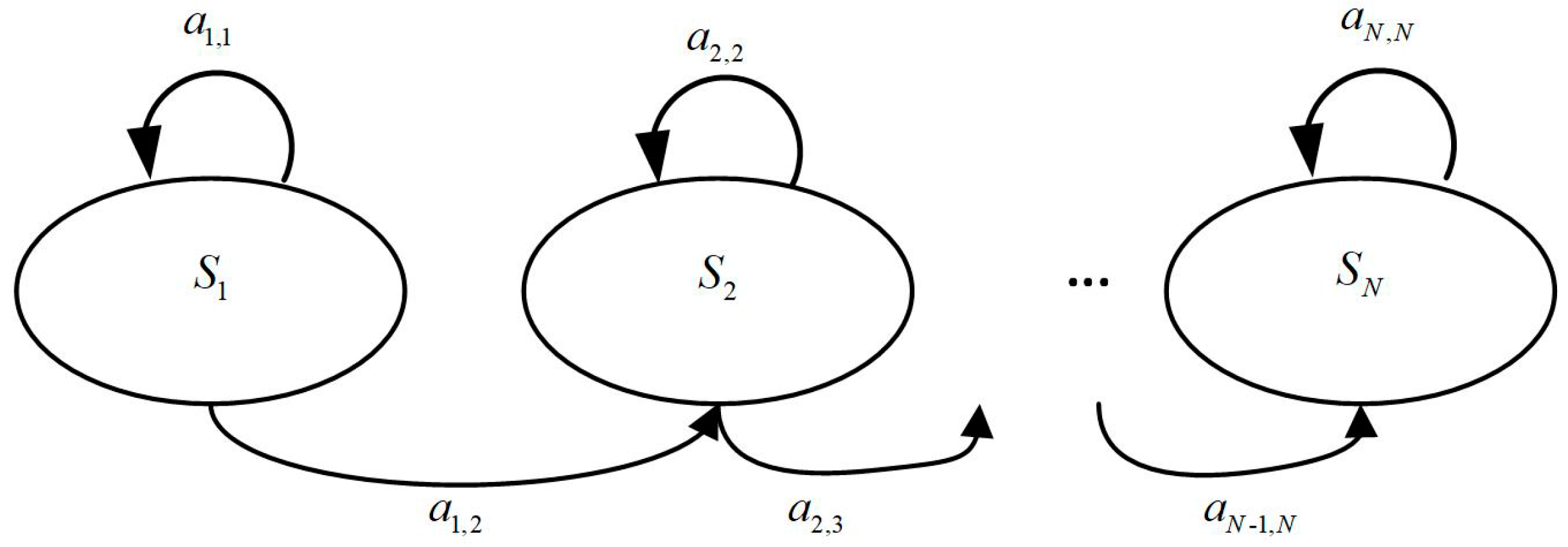
Considering that the degradation related to FED is time-variant, the random process with state duration can be used to describe the degrading process. The semi-Markov model is a typical statistic process widely used in reliability analysis when the residence time follows arbitrary distribution, which is thereby employed in this paper.
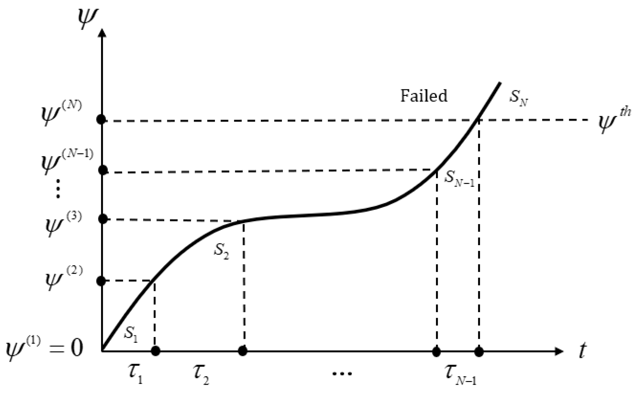
We assume a monotonous degrading process. Based on FED, the degrading process of an ETU can be decomposed into finite discrete states as shown in Figure 2. Assuming that the initial state of ETU is sound at , which is , at each time , the state satisfies the following:
where is the maximum energy dissipation, which means the ETU cannot meet the requirement of output energy. If at time , the state is , then there is a fixed transition probability that at the next time point , the state will be , which is:
The sojourn time in state may be expressed by a number of specific cycles (for example, the number of minutes, hours, days, or weeks), which is a random variable following any distribution [25]. Let be the sojourn time distribution, which is:
where k is an integer. The semi-Markov kernel can be obtained as:
Then, a semi-Markov model can be established, where is the initial state distribution, is the transition probability matrix composed by and is the sojourn time distribution of each state, which can be expressed as:
Based on Definition 2, the reliability of an ETU based on FED can be given as:
and can be obtained by the recursive method [26]:
2.3. Reliability Evaluation of Energy Transfer
An energy transfer system with ETUs transmits different types of energy and each ETU degrades under several possible degrading modes with various degrading paths. Particularly, the degradation of ETU is influenced by degrading mechanisms. The failure of the system is when the system cannot provide enough energy to implement a certain function, or the FED of the system exceeds failure threshold of the system . Then, the reliability of the target system can be obtained by:
where presents the FED generated by degrading mechanisms of ETU.
We should note that the convolutional function in Equation (16), which concerns the energy transfer capacity of the entire system, should be regarded as a global evaluating method. For a system with fixed topology, a traditional method for serial and parallel systems, with individual failure thresholds of each component, such as the block diagram method, can be conducted. In practice, the reliability of the system concerns the performance of the entire system and the threshold of a single component is not easily defined. The influence of the system structure is not explicitly shown by Equation (16). Instead, the work condition of each ETU in the system is influenced by the system structure, which will eventually change the FED and the reliability assessment result.
3. Parameters Estimation Using Probabilistic Physics-of-Failure Models
In Section 2, a multi-state reliability model of ETU, as well as the energy transfer system is established. The semi-Markov model is employed, which takes advantages of combining statistical reliability data with arbitrary sojourn time distribution. Statistically, all the parameters of the model can be estimated by sufficient data, which is used for reliability evaluation. Since FED is closely related to PPoF models, the parameters are possibly estimated with small sample sizes. In this section, parameters of the proposed model are estimated by mechanism instead of statistics.
The work stress of ETU can be load, pressure, flow, temperature and velocity and external environment may also influence the system, which results in different forms of degrading rates. Without loss of generality, we consider a time-varying incremental process to represent the physical degradation. The degrading rate is assumed to follow a Gaussian distribution, which is commonly utilized to describe the growth of cracks [27] and abrasive wear [28]. We should note that the degrading rate, which is based on a specific PPoF model, can be in arbitrary form. The increment of FED within a small-time duration should also follow a Gaussian distribution, which can be written as . Based on the specific degradation mechanism, degradation state can be divided by deterministic FED . Then, the FED at time can be derived as:
and the sojourn time of ith state can be expressed as:
where and are related to the specific form of and , respectively. Particularly, if the incremental process is a standard wiener process, and , otherwise, and can be obtained by the Monte-Carlo method. The probability density function of can be written as:
Considering the state transition model shown in Figure 3, the state keeps in the current state or transits to the next state. Assuming that at the state arrives at , given arbitrary time interval , the state transition probability can be written as:
and . The discrete sojourn time distribution can be written as:
Generally, with a deterministic PPoF model, the probability density function of τi can be derived. For different state transition models, the state transition probability and discrete sojourn time distribution follow a deterministic form. Then, the semi-Markov kernel can be obtained by Equation (12) and the reliability of ETU can be calculated by Equation (14).
4. Application in Electro-Hydrostatic Actuation System
The electro-hydrostatic actuation system (EHA) is a typical energy transfer system which drives external load by transferring electrical power to hydraulic power. In more electrical aircraft, EHA is used to drive control surfaces such as the aileron, elevator and rudder. Since EHA is used as the backup system, its failure may result in the aircraft going out of control. An EHA is composed of a high-speed motor, hydraulic pump and hydraulic cylinder, which are regarded as ETUs in this paper. The high-speed motor drives the rotation of the hydraulic pump, which provides high hydraulic pressure to drive the motion of the cylinder. The structure of EHA is shown in Figure 4.
An EHA fails when it cannot provide enough energy to drive the external load. The insufficiency of energy is the result of degradation on each ETU. The degradation of the motor will lead to a low input rotation speed and torque of the pump. The leakage of the pump results in lower driving pressure of the cylinder, and the degradation of the cylinder directly affects the output force of the system. For the pump, we consider three degradation mechanisms, which are leakage caused by abrasion between the piston and the plunger chamber, leakage caused by abrasion between the cylinder barrel and the valve plate, and leakage caused by abrasion between the slipper and swash plate. For the motor, we view decreasing output torque as wear between the bearing rings and bearing ball. For the cylinder, we consider the leakage caused by wear of seals. We should note that the degradation mechanisms considered in this paper may cover the major energy loss caused by wear, but are far from complete, due to the limitation of the authors’ knowledge. It is mainly used to illustrate the proposed method and some of the assumptions are different from practice. PPoF models for ETUs are firstly built in Section 4.1, Section 4.2, Section 4.3, and the proposed method is conducted to analyze the reliability of the system in Section 4.4.
4.1. Probabilistic Physics-of-Failure Model for Hydraulic Pump Degradation
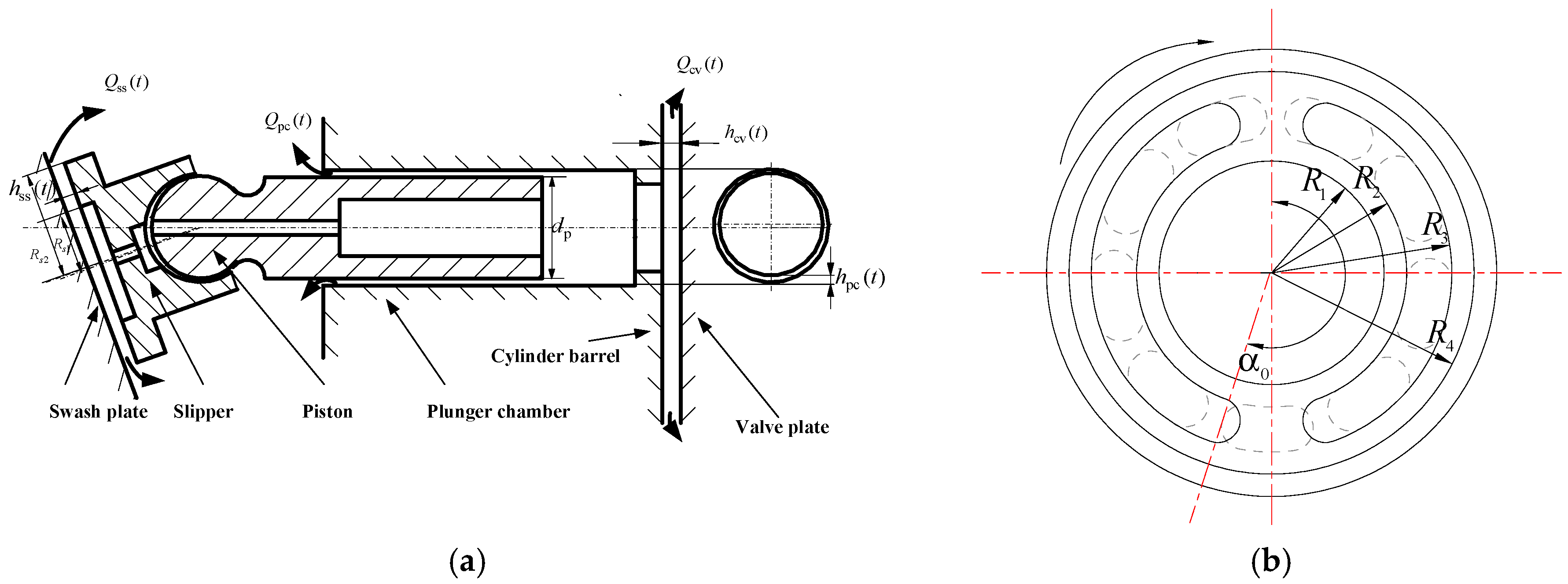
In an aviation EHA, the axial piston pump is used to transfer energy from the electrical motor to the hydraulic cylinder. According to the statistic survey, the main failure of the piston pump is wearing and tearing of friction pairs, as shown in Figure 5. Since the degradation of the piston pump failure goes through the stages of lubrication, boundary lubrication and friction wear, its failure mechanism-based model needs describe all of the above process. When wear produces abrasive particles between the friction pairs of the piston pump, the increased wear leads to leakage between the friction pairs. At this moment, it is difficult to provide the required flow rate to the downstream component. There are three friction pairs in the piston pump, which are the valve-plate–cylinder-barrel, the slipper–swash plate and the piston–plunger chamber. Their wear and tear cause more than 95% leakage during the pump running [29] in real application.
Here we select the valve-plate–cylinder-barrel to indicate how to establish the failure mechanism-based model considering the degradation process. Because the piston pump goes through the lubrication, boundary lubrication and wear process during the degradation, the pressure distribution and the oil film distribution vary with the time, and thus the leakage flow can be calculated when the dimensional parameters of the valve plate , , and are fixed by [28]:
where is the angle distribution of the pistons, is the suction pressure, is the discharge pressure, is the dynamic viscosity and is the average clearance between the cylinder barrel and the valve plate. During the working process of the pump, the surfaces of the cylinder-barrel–valve-plate are not directly contacted, so that the surfaces are separated by a thin lubricating oil film. When there is no contaminant, the thickness of the lubricating oil film is equal to the clearance between the cylinder barrel and the valve plate. The abrasion will lead to a larger average clearance and the degradation rate of leakage can be obtained by .
Based on the definition of FED, the fluid energy of the leakage can be roughly regarded as the dissipation energy of the degradation caused by the abrasion between cylinder barrel and valve plate when the thermal effect is ignored. Assuming that the pump is working under pressure , the corresponding FED can be calculated as:
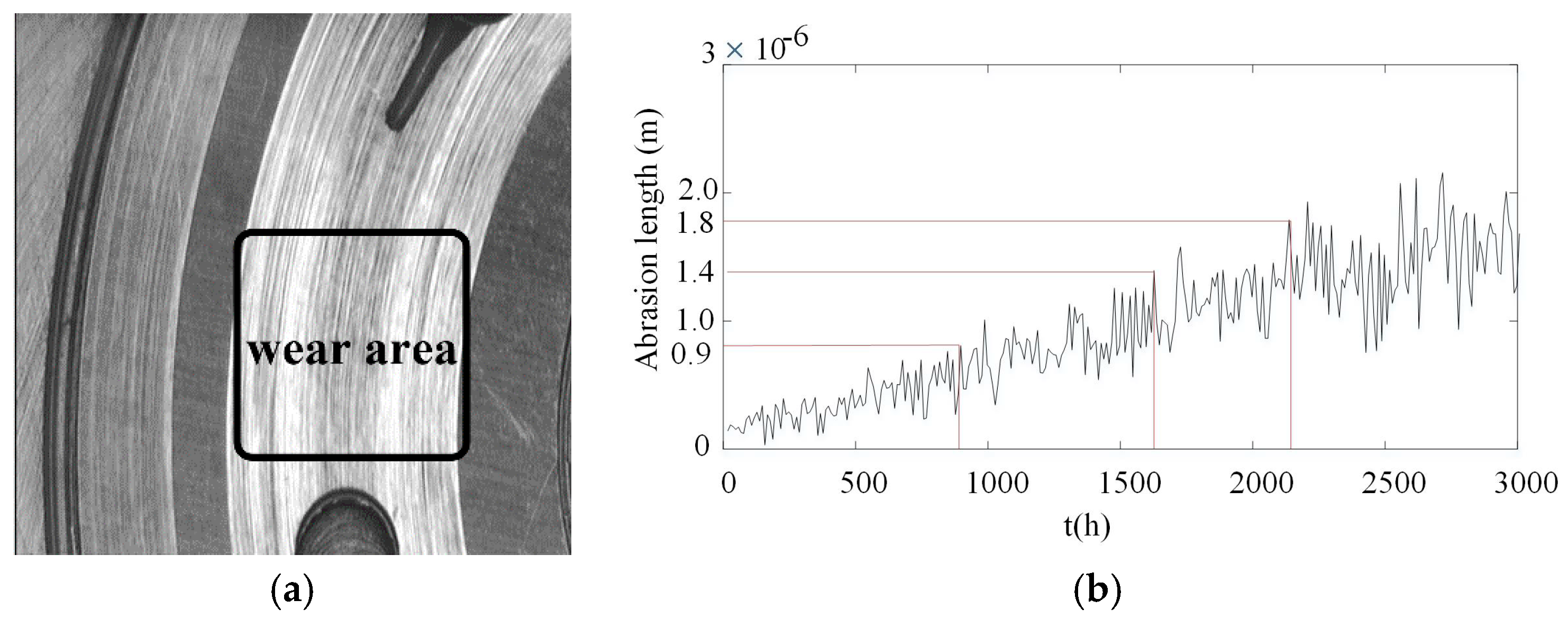
We consider a three-body abrasive wear process to illustrate a possible way to obtain the degradation rate. A relevant research study [30] shows that the degree of wear caused by particles is mainly affected by the size of debris particles and the distance between the two surfaces. As is shown in Figure 6a, the scratch of valve plate is probably caused by the invasion of a debris particle. The measurement data of the abrasion length is shown in Figure 6b.
Based on the research by Dwyer-Joyce [31], assuming that the debris particles follow Gaussian distribution, the increment of the average clearance can be expressed as , and:
where is the nominal contact area, is the rotating speed of pump, is the relative hardness of the two contact surfaces, and are the parameters of debris loss rate, and the expression of and which are related to the dimensional parameters of pump and distributions of debris particles is shown in Appendix A. We should note that such a model neglects the energy cost of material fracture, frictional sliding and the flow loss caused by the invasion of debris, which takes a low percentage.
Similarly, the FED caused by the other two degradation mechanisms can be obtained. According to the study by Wang [28], the leakage caused by the friction pair of piston and plunger chamber can be calculated by
where is the eccentricity ratio, is the relative velocity of the two contact surfaces, is the diameter of the piston, is the piston length and is the average clearance of the two surfaces. The increasing leakage can be obtained when the average clearance of the two surfaces changes. The leakage caused by the friction pair of slipper and swash plate can be calculated by:
where is the pressure in the slipper center hole, and are the dimensional parameters shown in Figure 5, and is the average clearance of the two surfaces. Then the FED of the pump by the three degradation mechanisms can be obtained by:
4.2. Probabilistic Physics-of-Failure Model for Motor Degradation
The motor drives the rotation pump by converting electrical energy into mechanical energy. The degradation of the motor is mainly reflected by the decreasing of output torque and speed. Based on different control methods, the motor can maintain its output by increasing input energy when degradation occurs, which results in lower efficiency. The degradation may be caused by the magnetic components or mechanical components. In this part, we only consider the decreasing output torque by wear between the bearing rings and bearing balls of an angular contact ball bearing (ACBB).
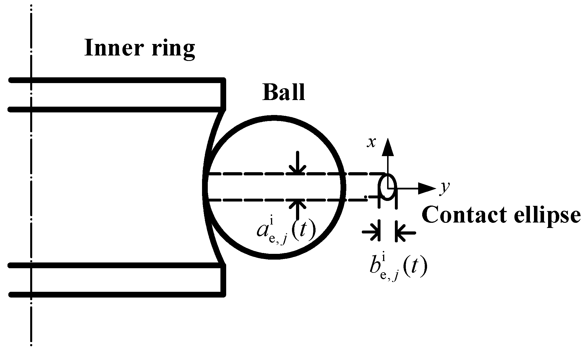
With the operation of the motor, a degrading ACBB will generate additional friction torque. This part of torque can be regarded as the reduction of rated output torque. According to the characteristics of internal friction in ACBB, the additional friction torque is mainly caused by the elastic hysteresis between ball and the rings, the fluid dynamic pressure and the effect of differential sliding. The study result by Deng et al. [32] is employed to illustrate how to establish the relation between FED and PPoF models of decreasing output torque by wear between the bearing rings and bearing balls, considering two-body wear between balls and rings. On the basis of dynamic analysis [33], the hysteresis energy through a loading cycle for the (total number of balls is ) ball can be written as:
where is the elastic hysteresis coefficient, is the rotating speed, is the revolution speed of the ball, is the contact load between each ball and the ring, and are the Poisson’s ratio of balls and rings, and are the elastic modulus of balls and rings, is the ellipticity of contact ellipse, which is shown in Figure 7, is the distance from the ball to the rotary shaft, is the sum of curvatures, is complete elliptic integral of the first kind on the contact ellipse, is the complete elliptic integral of the second kind on the contact ellipse and the superscript and represent the inner ring (cone) and outer ring (cup), respectively. The torque reduction by the hysteresis energy can be calculated as:
The energy cost by fluid dynamic pressure can be calculated by:
where is the oil film thickness, is the viscosity of oil, is the fluid dynamic pressure, is the relative velocity of the ball and inner ring and is the relative velocity of the ball and outer ring. The torque reduction by fluid dynamic pressure can be calculated as:
The energy cost by the effect of differential sliding can be calculated by:
where is the friction coefficient between balls and rings, is the differential sliding velocity, is the contact ellipse area. The torque reduction by the effect of differential sliding can be calculated as:
The total reductive torque can be calculated as:
and the corresponding FED can be given as:
where is the rotating speed of the motor.
We consider a two-body wear between the ball and rings. Particularly, we assume that the wear performs uniformly on the balls, and that the balls remain isotropous during the wear. The two-body wear leads to a reduction on the radius of the balls. Since the two-body wear is a stochastic process, which is influenced by rough contact surfaces and the environment, the wear rate, which depicts the radius change of the ball, is assumed to follow a certain distribution.
The change of the sum of curvatures can then be obtained by:
where is the radius of the ball, is the radius of inner ring and is the radius of outer ring. Based on Hertz theory, the parameter of the contact ellipse can be calculated by:
where is the contact pressure, and are related to the dimensional parameters of the bearing. We should note that such a model neglects the deformation of rings, the wear of rings and the energy cost during the wear process.
4.3. Probabilistic Physics-of-Failure Model for Hydraulic Cylinder Degradation
The hydraulic cylinder, working as the actuator in EHA, outputs the terminal energy to external loads. The degradation of the hydraulic cylinder leads to the decreasing of output force. The dynamic seals move with the piston of the cylinder, as shown in Figure 8. A vital degradation mode is the internal leakage, caused by the wear of dynamic seals, which makes the pressure difference between the high-pressure chamber and the low-pressure chamber decrease. The internal leakage will, then, cause the reduction of output force.
We consider the internal leakage caused by the wear of dynamic seals. The total internal leakage of the cylinder can be calculated by [34]:
where is the clearance between the seal and the cylinder barrel, is the contact width of seal and cylinder along axial direction, is the contact length of seal and cylinder, is the kinematic viscosity and is the percolation channel shape correction coefficient.
By introducing Archard’s equation, the clearance between the seal and the cylinder barrel can be calculated by:
where is the wear efficient, is the hardness of seal, is the contact pressure between the seal and the cylinder barrel. The details to obtain is derived in Appendix B. The FED can be obtained by:
Since the wear process is influenced by topology of the rough contact surfaces, the contact pressure between the seal and the piston is assumed to follow a certain distribution.
4.4. Reliability Evaluation of Electro-Hydrostatic Actuation System
The target scenario is to use a certain type of EHA [35] to drive a control surface of an aircraft independently. The rated output power of the EHA is 10 kW, the rated hydraulic pressure is 28 MPa and the rated motor rotation speed is 12,000 r/min. According to the energy requirement listed in [36,37], the minimum power requirement for an aileron during a regular flight is approximate 8 kW. Assuming that the rated efficient of the EHA is 90%, the FED threshold of the system is estimated at 2.2 kW.
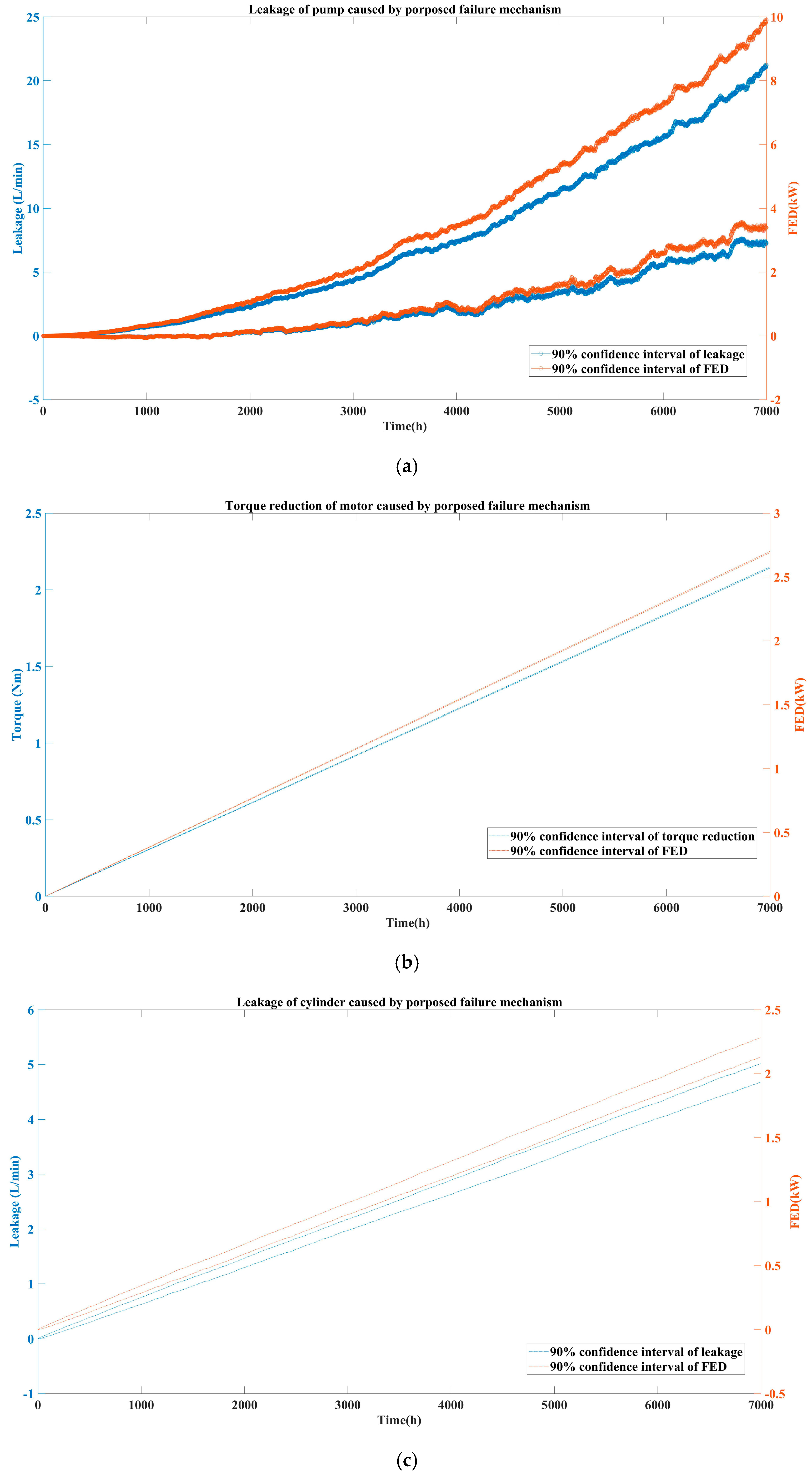
The details of the uncertainty for the considered scenario is shown in Table 1, which has been configured by the author, according to [32,34,38]. The degradation rate of each variable has been normalized to each minute. For an intuitive degradation process, a Monte-Carlo simulation is conducted. The degradation process of each ETU is illustrated by 1000 samples under the proposed uncertainty configuration. As shown in Figure 9, 90% confidence interval of all the 1000 samples at each time point is calculated, and the FED corresponding to the specific failure mechanism is shown with the degradation process of each ETU.
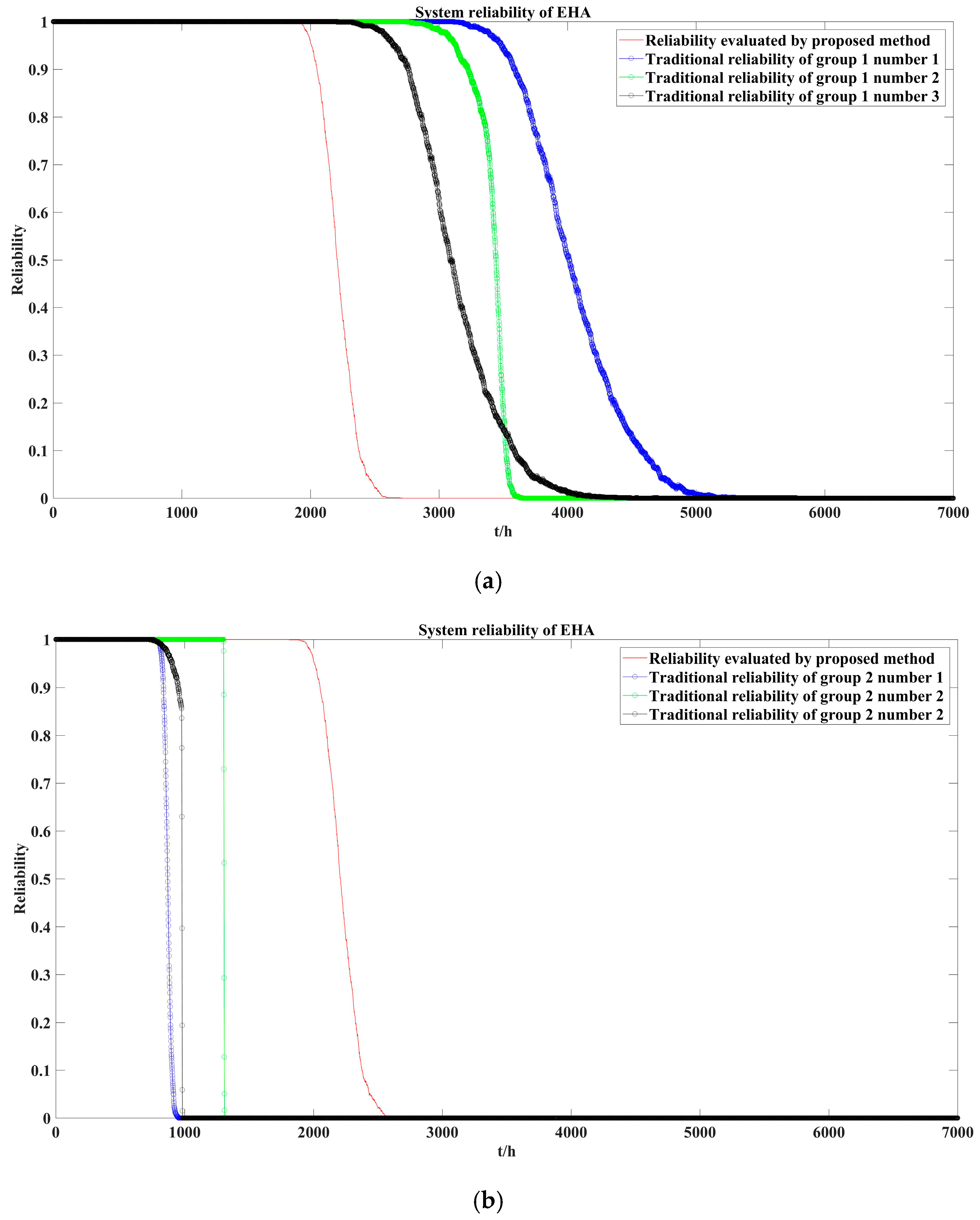
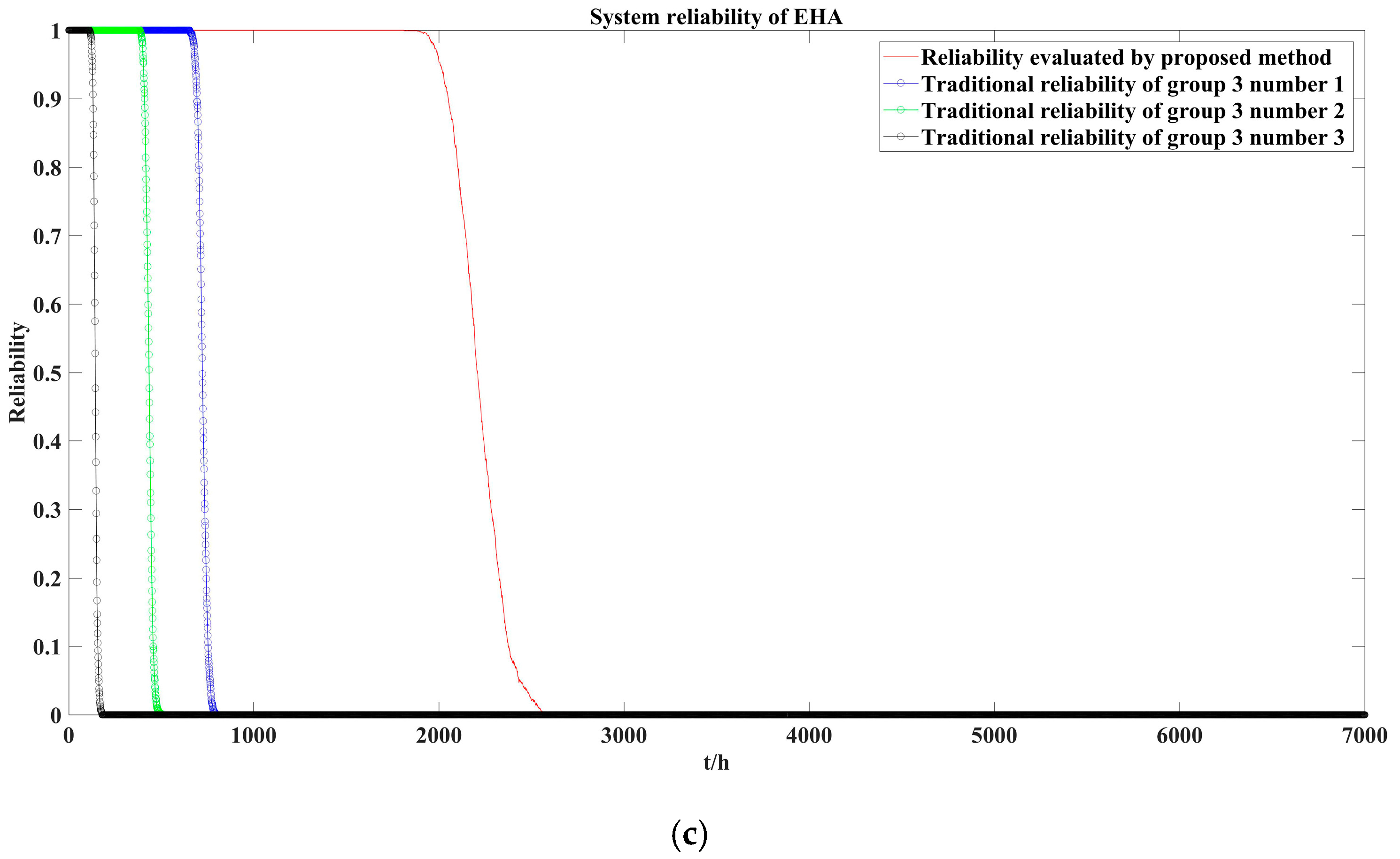
If the system is evaluated by the criterion that the system fails when the FED of the system reaches 2.2 kW, then the reliability of the system can be obtained by the proposed method. To compare with the traditional evaluating method, the criterion of which is defined by failure thresholds of individual components, the individual failure thresholds are defined as , and , respectively. In traditional methods, in fact, the failure data and failure thresholds are obtained by reliability test. Hereby, traditional thresholds of given components are referred to, and configured by, the author. The traditional reliability of the serial system can thus be obtained by:
where is the torque reduction of motor, is the leakage of pump and is the leakage of cylinder.
A total of 3 groups of comparisons are conducted to show the difference between traditional reliability assessment methods using individual failure thresholds, and the proposed system-level method. For the first group, the summation of equivalent FED of each individual failure threshold is set to be larger than the system threshold 2.2 kW. For the second group, the summation of the equivalent FED of each individual failure threshold is set to be around the system threshold. For the third group, the summation FED of each individual failure threshold is set to be less than the system threshold. The detailed simulation data are listed in Table 2.
With different individual failure thresholds, the reliability evaluated by the individual failure thresholds are shown in Figure 10. We can see that in Figure 10a, when the summation of equivalent FED of each individual threshold is larger than the system FED threshold, the reliability evaluated by the traditional method has a greater margin than the proposed method, which is in accordance with the fact that larger thresholds mean more tolerance of degradation. In Figure 10c, when the summation of the equivalent FED of each individual threshold is less than the system FED threshold, then the reliability evaluated by the traditional method has a smaller margin than the proposed method. For group 2, the traditional method has less tolerance of degradation than the proposed method, which can be explained by the fact that, although the pump has already met the presupposed threshold, for the system, it can still be used. On this basis, the proposed method is less rigorous than the traditional method, when the summation of equivalent FED equals the system FED threshold.
From the figures, we can also see that the reliability evaluated by the traditional method sharply decreases when the summation of the equivalent FED is relatively small. This is related to the uncertainty configuration. Since under a smaller threshold of failure, the reliability is more likely to be influenced by the components with fewer uncertainties, in the PPoF models established in the above sections, the modeling uncertainty of the motor is weakened by the assumption of the uniform wear process, which leads to the dominance of the motor when the summation of equivalent FED is relatively small.
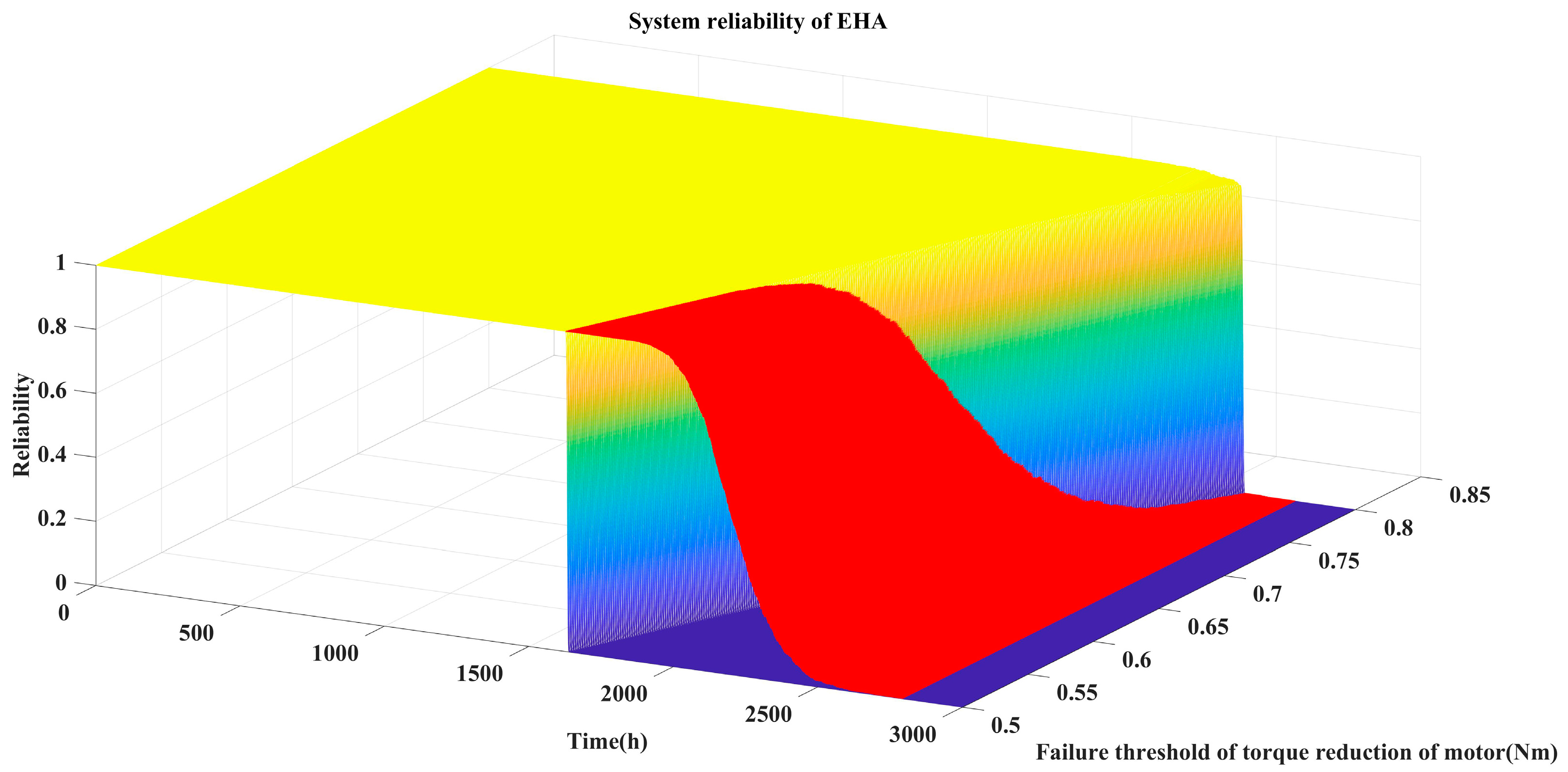
As a global criterion, the reliability evaluated by the system failure threshold can help ascertain the traditional thresholds of individual components. In fact, the ascertaining traditional thresholds of individual components is a dynamic process. By setting the thresholds of the pump and the cylinder fixed at L/min and L/min, the traditional reliability can be calculated by changing the threshold of the motor. As shown in Figure 11, the red surface is the reliability evaluated by the proposed method, which is only dependent on time, meanwhile, the other surface, which presents the traditional reliability, depends on both time and the individual failure threshold of the motor. The intersecting curve of the two surfaces can be used to ascertain the failure thresholds of the motor, with fixed thresholds of the pump and the cylinder. By using such a method, it can effectively avoid the scenario where, despite the motor already meeting the presupposed threshold, the system continues to provide enough output, which will prolong the service life and will provide potential economic benefits.
5. Conclusions
A system-level reliability assessment method for the energy transfer system is proposed in this paper to solve the practical difficulty of a unified description of the system degradation state, caused by different physical degradation mechanisms. FED is an additive variable to quantitatively evaluate the effect of component degradation on the entire system. PPoF models of different mechanisms can be used to obtain the corresponding FED. By using FED, the system reliability can be defined from the perspective of the system, instead of using a set of individual failure thresholds of components. An application in EHA shows that the proposed method is effective for describing system reliability and the method can help ascertain the component failure threshold when the system threshold is confirmed.
It is worth noting that, although in this paper wear processes of different EHA components are modeled and FED is obtained, the other degradation mechanisms such as electrical, magnetic and chemical mechanisms could also be modeled, and the corresponding FED can be obtained in a similar way. Since there is no common method to build the PPoF models, sufficient knowledge of studied degradation mechanisms is required to establish the relation between uncertainties and system dynamics. In this paper, we consider some uncertainties which are modeled as certain distributions and make assumptions to avoid some uncertainties, but there are still uncertainties that are not recognized by the authors. With the development of knowledge, there will be more and more uncertainties being transformed to certainties. For unknown degradation mechanisms, the statistical reliability data can be used to describe the state transition model of the degrading process, alternatively.
Author Contributions
X.C. and T.L. wrote the manuscript together; S.W. designed the idea and provided supervision; J.S. reviewed the manuscript.
Funding
This research was funded by National Natural Science Foundation of China (51875014, 51575019, 51620105010), Natural Science Foundation of Beijing Municipality (L171003) and Program 111 of China.
Conflicts of Interest
The authors declare no conflict of interest.
Abbreviations
| PoF | Physics of failure |
| PPoF | Probabilistic physics-of-failure |
| EHA | Electro-hydrostatic actuation system |
| FED | Failure related energy dissipation |
| ETU | Energy transmission unit |
| ACBB | Angular contact ball bearings |
Appendix A
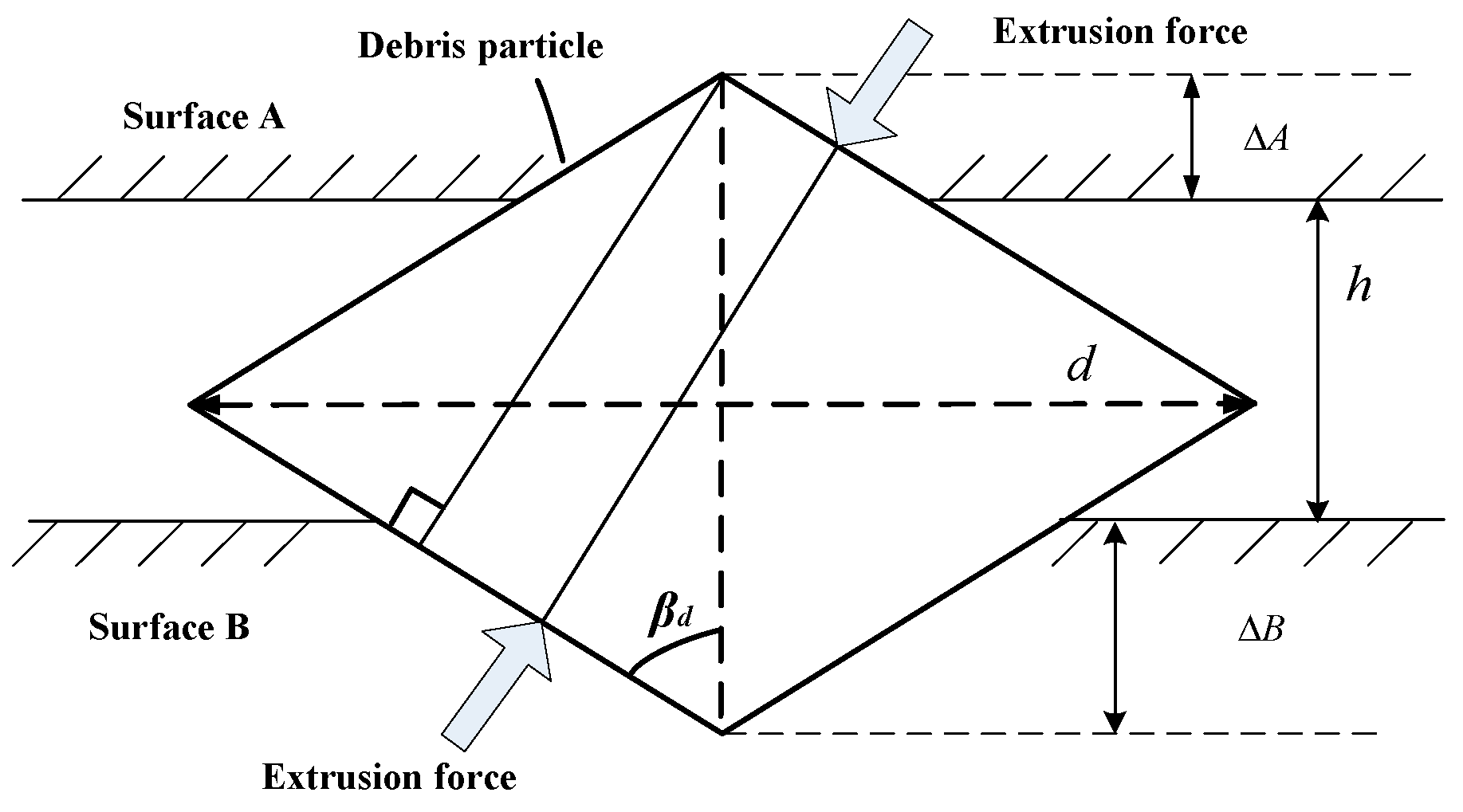
According to the two-dimensional diamond abrasive particle model proposed by Williams and Hyncica [39], the three-body abrasive wear can be assumed to be caused by an idealized debris particle, as shown in Figure A1. stands for the maximum width of a particle, is shape angle of the particle and is the oil film thickness. and are the depth of debris particles embedded in the upper and lower surface, respectively. According to the requirement of working oil contamination for the aviation hydraulic pump, the oil contamination should satisfy the standard according to NAS 1638, which is listed in Table A1.
Figure A1.
Schematic diagram of abrasive wear under lubrication condition.


Table A1.
Particle concentration of Grade 8 (number of particles in 100 mL).
| 5–15 | 15–25 | 25–50 | 50–100 | >100 | |
|---|---|---|---|---|---|
| Number of particles | 64,000 | 11,400 | 2025 | 360 | 64 |
We can see from Table A1 that the majority of the debris particles are small ones. If the clearance of the two surfaces is larger than the size of the debris, then considering the influence by shape, , there is less probability for abrasion. Since the hardness of the two contact surfaces is different, three possible conditions may result in different degrees of damage on the surfaces. If the size of a debris particle is larger than the clearance and the hardness of debris is smaller than both surfaces, the abrasion is ignored. If the hardness of debris is larger than one of the two surfaces, the abrasion only occurs on the soft surface. If the hardness of debris is larger than both surfaces, the damage ratio is proportional to the relative hardness of the two surfaces. The wear volume caused by the debris particles, with specific concentration and distribution during one stress cycle of the friction pair can be used to calculate the increment of average clearance by dividing the nominal contact area of the two surfaces.
Assuming that the hardness of debris is larger than both surfaces, the abrasion occurs on both surfaces. The wear depth caused by the debris can be obtained by:
The scratch area can be calculated as:
According to the experimental result, the thickness of oil film distributes as a sinewave along the circumference of the clearance:
where is the film thickness of outer seal oil zone, is the film thickness of inner seal oil zone, , and are the fitted parameters of the outer seal oil zone, , and are the fitted parameters of the inner seal oil zone. The total wear volume caused by this form of debris for one rotation cycle is:
where , , , , is the concentration of debris, is the probability that the debris flow away during the rotating, is the average oil volume in outer seal oil zone and is the average oil volume in inner seal oil zone.
If the debris loss rate , debris of different sizes which are larger than clearance all follow different Gaussian distributions where stands for kind of debris, the total wear volume follow a Gaussian distribution:
where
, and are obtained from Equation (A4):
where is the concentration of kind of debris.
Appendix B
The following derivation is based on the method proposed in [34]. The aim of this section is to get in Equation (39). Assuming that the seal is purely elastic and deformed, based on Hertzian contact theory, with a maximum peak squeezing stress , then the contact width of the seal and the cylinder along the axial direction can be calculated by:
where is the compressive displacement, is the diameter of the groove, is the diameter of seal, is the inside diameter of the cylinder, is the normalized squeeze and is the elastic modulus of seal, as shown in Figure A2.
Figure A2.
Schematic diagram of seal.

The peak squeezing stress can be calculated by:
Then, the total squeezing stress along axial direction can be calculated by:
and the stress on the entire contact area can be obtained by:
The contact pressure can be calculated by:
where is the contact area. Assuming that every point on the seal’s external surface has the same opportunity to be subject to wear, the diameter of seal can be updated by:
By substituting the updated diameter of seal into Equation (A8), the pressure per unit area can be obtained iteratively.
References
- Wang, K.; Wang, S.; Shi, J. A novel multi-state reliability assessment model for servo HA/EHA system via universal generating function. In Proceedings of the 2017 IEEE International Conference on Mechatronics and Automation (ICMA), Takamatsu, Japan, 6–9 August 2017; IEEE: Piscataway, NJ, USA, 2017; pp. 1918–1923. [Google Scholar]
- Jafary, B.; Fiondella, L. A universal generating function-based multi-state system performance model subject to correlated failures. Reliab. Eng. Syst. Saf. 2016, 152, 16–27. [Google Scholar] [CrossRef]
- Lisnianski, A.; Levitin, G.; Ben-Haim, H.; Elmakis, D. Power system structure optimization subject to reliability constraints. Electr. Power Syst. Res. 1996, 39, 145–152. [Google Scholar] [CrossRef]
- Chen, H.P.; Mehrabani, M.B. Reliability analysis and optimum maintenance of coastal flood defences using probabilistic deterioration modelling. Reliab. Eng. Syst. Saf. 2019, 185, 163–174. [Google Scholar] [CrossRef]
- Dhawalikar, M.N.; Mariappan, V.; Srividhya, P.; Kurtikar, V. Multi-state failure phenomenon and analysis using semi-Markov model. Int. J. Qual. Reliab. Manag. 2018, 35, 2080–2091. [Google Scholar] [CrossRef]
- Wang, W.; Di Maio, F.; Zio, E. A sensitivity analysis for the adequacy assessment of a multi-state physics modeling approach for reliability analysis. In Proceedings of the 26th European Safety and Reliability Conference, ESREL 2016, Glasgow, UK, 25–29 September 2016; CRC Press/Balkema: Leiden, The Netherlands, 2017; pp. 465–472. [Google Scholar]
- IEEE. IEEE Standard 1413.1-2002, IEEE Guide for Selecting and Using Reliability Predictions Based on IEEE 1413; The Institute of Electrical and Electronics Engineers Inc.: New York, NY, USA, 2003. [Google Scholar]
- Sun, B.; Fan, X.; Qian, C.; Zhang, G. PoF-simulation-assisted reliability prediction for electrolytic capacitor in LED drivers. IEEE Trans. Ind. Electron. 2016, 63, 6726–6735. [Google Scholar] [CrossRef]
- Ma, K.; Wang, H.; Blaabjerg, F. New approaches to reliability assessment: Using physics-of-failure for prediction and design in power electronics systems. IEEE Power Electron. Mag. 2016, 3, 28–41. [Google Scholar] [CrossRef]
- Zeng, Z.; Kang, R.; Chen, Y. Using PoF models to predict system reliability considering failure collaboration. Chin. J. Aeronaut. 2016, 29, 1294–1301. [Google Scholar] [CrossRef] [Green Version]
- Modarres, M.; Amiri, M.; Jackson, C. Probabilistic Physics of Failure Approach to Reliability: Modeling, Accelerated Testing, Prognosis and Reliability Assessment; John Wiley & Sons: Hoboken, NJ, USA, 2017. [Google Scholar]
- Modarres, M.; Kaminskiy, M.P.; Krivtsov, V. Reliability Engineering and Risk Analysis: A Practical Guide; CRC Press: Boca Raton, FL, USA, 2016. [Google Scholar]
- Distefano, S.; Puliafito, A. Dependability evaluation with dynamic reliability block diagrams and dynamic fault trees. IEEE Trans. Dependable Secur. Comput. 2009, 6, 4–17. [Google Scholar] [CrossRef]
- Čepin, M.; Mavko, B. A dynamic fault tree. Reliab. Eng. Syst. Saf. 2002, 75, 83–91. [Google Scholar] [CrossRef]
- Robidoux, R.; Xu, H.; Xing, L.; Zhou, M. Automated modeling of dynamic reliability block diagrams using colored Petri nets. IEEE Trans. Syst. Man Cybern. Part A Syst. Hum. 2009, 40, 337–351. [Google Scholar] [CrossRef]
- Rao, K.D.; Gopika, V.; Rao, V.S.; Kushwaha, H.; Verma, A.K.; Srividya, A. Dynamic fault tree analysis using Monte Carlo simulation in probabilistic safety assessment. Reliab. Eng. Syst. Saf. 2009, 94, 872–883. [Google Scholar]
- Wang, S.; Cui, X.; Shi, J.; Tomovic, M.M.; Jiao, Z. Modeling of reliability and performance assessment of a dissimilar redundancy actuation system with failure monitoring. Chin. J. Aeronaut. 2016, 29, 799–813. [Google Scholar] [CrossRef] [Green Version]
- Wang, Y.; Pham, H. Modeling the dependent competing risks with multiple degradation processes and random shock using time-varying copulas. IEEE Trans. Reliab. 2011, 61, 13–22. [Google Scholar] [CrossRef]
- Yang, Z.; Zhao, J.; Cheng, Z.; Li, L. Reliability Modeling of Two-Component System with Degradation Interaction Based on Copulas. In Proceedings of the 2018 Prognostics and System Health Management Conference (PHM-Chongqing), Chongqing, China, 26–28 October 2018; IEEE: Piscataway, NJ, USA, 2018; pp. 138–143. [Google Scholar]
- Wu, X.; Hillston, J. Mission reliability of semi-Markov systems under generalized operational time requirements. Reliab. Eng. Syst. Saf. 2015, 140, 122–129. [Google Scholar] [CrossRef] [Green Version]
- Wu, B.; Cui, L.; Fang, C. Reliability Analysis of Semi-Markov Systems with Restriction on Transition Times. Reliab. Eng. Syst. Saf. 2019, 190, 106516. [Google Scholar] [CrossRef]
- Archard, J. Contact and rubbing of flat surfaces. J. Appl. Phys. 1953, 24, 981–988. [Google Scholar] [CrossRef]
- Pugno, N.; Ciavarella, M.; Cornetti, P.; Carpinteri, A. A generalized Paris’ law for fatigue crack growth. J. Mech. Phys. Solids 2006, 54, 1333–1349. [Google Scholar] [CrossRef]
- Laidler, K.J. The development of the Arrhenius equation. J. Chem. Educ. 1984, 61, 494. [Google Scholar] [CrossRef]
- Chryssaphinou, O.; Limnios, N.; Malefaki, S. Multi-state reliability systems under discrete time semi-Markovian hypothesis. IEEE Trans. Reliab. 2011, 60, 80–87. [Google Scholar] [CrossRef]
- Veeramany, A.; Pandey, M.D. Reliability analysis of nuclear component cooling water system using semi-Markov process model. Nucl. Eng. Des. 2011, 241, 1799–1806. [Google Scholar] [CrossRef]
- Birnbaum, Z.W.; Saunders, S.C. A new family of life distributions. J. Appl. Probab. 1969, 6, 319–327. [Google Scholar] [CrossRef]
- Wang, X.; Lin, S.; Wang, S.; He, Z.; Zhang, C. Remaining useful life prediction based on the Wiener process for an aviation axial piston pump. Chin. J. Aeronaut. 2016, 29, 779–788. [Google Scholar] [CrossRef] [Green Version]
- Tongyang, L.I.; Wang, S.; Shi, J.; Zhonghai, M.A. An adaptive-order particle filter for remaining useful life prediction of aviation piston pumps. Chin. J. Aeronaut. 2018, 31, 941–948. [Google Scholar]
- Roylance, B.; Williams, J.; Dwyer-Joyce, R. Wear debris and associated wear phenomena—Fundamental research and practice. Proc. Inst. Mech. Eng. Part J J. Eng. Tribol. 2000, 214, 79–105. [Google Scholar] [CrossRef]
- Dwyer-Joyce, R. Predicting the abrasive wear of ball bearings by lubricant debris. Wear 1999, 233, 692–701. [Google Scholar] [CrossRef]
- Sier, D.; Xinglin, L.; Jiugen, W. Analysis on the friction torque fluctuation of angular contact ball bearings. J. Mech. Eng. 2011, 47, 104–112. [Google Scholar]
- Biboulet, N.; Houpert, L. Hydrodynamic force and moment in pure rolling lubricated contacts. Part 1: Line contacts. Proc. Inst. Mech. Eng. Part J J. Eng. Tribol. 2010, 224, 765–775. [Google Scholar] [CrossRef]
- Cao, Y.; Dai, X. Modeling for performance degradation induced by wear of a hydraulic actuator of a hydraulic excavator. Proc. Inst. Mech. Eng. Part C J. Mech. Eng. Sci. 2015, 229, 556–565. [Google Scholar] [CrossRef]
- Rongjie, K.; Zongxia, J.; Shaoping, W.; Lisha, C. Design and simulation of electro-hydrostatic actuator with a built-in power regulator. Chin. J. Aeronaut. 2009, 22, 700–706. [Google Scholar] [CrossRef]
- Chakraborty, I.; Trawick, D.R.; Mavris, D.N.; Emeneth, M.; Schneegans, A. A requirements-driven methodology for integrating subsystem architecture sizing and analysis into the conceptual aircraft design phase. In Proceedings of the 14th AIAA Aviation Technology, Integration, and Operations Conference, Atlanta, GA, USA, 16–20 June 2014; p. 3012. [Google Scholar]
- Chakraborty, I.; Mavris, D.N.; Emeneth, M.; Schneegans, A. A system and mission level analysis of electrically actuated flight control surfaces using Pacelab SysArc. In Proceedings of the 52nd Aerospace Sciences Meeting, National Harbor, MD, USA, 13–17 January 2014; p. 0381. [Google Scholar]
- Du, J.; Wang, S.; Zhang, H. Layered clustering multi-fault diagnosis for hydraulic piston pump. Mech. Syst. Signal Process. 2013, 36, 487–504. [Google Scholar] [CrossRef]
- Williams, J.; Hyncica, A. Mechanisms of abrasive wear in lubricated contacts. Wear 1992, 152, 57–74. [Google Scholar] [CrossRef]
Figure 1.
General model of energy transmission unit (ETU).

Figure 2.
Degrading process of an ETU.

Figure 3.
State transition model.

Figure 4.
Schematic structure of electro-hydrostatic actuator.

Figure 5.
Schematic structure of three main friction pairs: (a) three main friction pairs; (b) valve plate.
Figure 5.
Schematic structure of three main friction pairs: (a) three main friction pairs; (b) valve plate.

Figure 6.
Physical failure process of a valve plate: (a) the scratch of valve plate; (b) abrasion length.
Figure 6.
Physical failure process of a valve plate: (a) the scratch of valve plate; (b) abrasion length.

Figure 7.
The contact between ball and inner ring of angular contact ball bearing (ACBB).

Figure 8.
Schematic structure of cylinder.

Figure 9.
Degradation process of each ETU with 90% confidence interval: (a) pump; (b) motor; (c) cylinder.
Figure 9.
Degradation process of each ETU with 90% confidence interval: (a) pump; (b) motor; (c) cylinder.

Figure 10.
Reliability of electro-hydrostatic actuation system (EHA): (a) simulation result of group 1; (b) simulation result of group 2; (c) simulation result of group 3.
Figure 10.
Reliability of electro-hydrostatic actuation system (EHA): (a) simulation result of group 1; (b) simulation result of group 2; (c) simulation result of group 3.


Figure 11.
Failure related energy dissipation (FED) distribution with different individual failure thresholds.
Figure 11.
Failure related energy dissipation (FED) distribution with different individual failure thresholds.

Table 1.
Uncertainty configuration.
| ETU | Degradation Variable | Distribution Type of Degradation Rate | Related Parameters | Failure Threshold |
|---|---|---|---|---|
| Pump | Leakage (L/min) | Gaussian | ||
| Motor | Torque reduction (Nm) | Uniform | ||
| Cylinder | Leakage (L/min) | Gaussian |
Table 2.
Individual failure thresholds.
| Group | Number | Individual Failure Thresholds | Summation of Equivalent FED |
|---|---|---|---|
| 1 | 1 | L/min, Nm and L/min | 6.68 kW |
| 2 | L/min, Nm and L/min | 4.75 kW | |
| 3 | L/min, Nm and L/min | 5.79 kW | |
| 2 | 1 | L/min, Nm and L/min | 2.207 kW |
| 2 | L/min, Nm and L/min | 2.213 kW | |
| 3 | L/min, Nm and L/min | 2.201 kW | |
| 3 | 1 | L/min, Nm and L/min | 1.91 kW |
| 2 | L/min, Nm and L/min | 1.56 kW | |
| 3 | L/min, Nm and L/min | 0.98 kW |
© 2019 by the authors. Licensee MDPI, Basel, Switzerland. This article is an open access article distributed under the terms and conditions of the Creative Commons Attribution (CC BY) license (http://creativecommons.org/licenses/by/4.0/).
Share and Cite
MDPI and ACS Style
Cui, X.; Wang, S.; Li, T.; Shi, J. System Reliability Assessment Based on Energy Dissipation: Modeling and Application in Electro-Hydrostatic Actuation System. Energies 2019, 12, 3572. https://0-doi-org.brum.beds.ac.uk/10.3390/en12183572
AMA Style
Cui X, Wang S, Li T, Shi J. System Reliability Assessment Based on Energy Dissipation: Modeling and Application in Electro-Hydrostatic Actuation System. Energies. 2019; 12(18):3572. https://0-doi-org.brum.beds.ac.uk/10.3390/en12183572
Chicago/Turabian StyleCui, Xiaoyu, Shaoping Wang, Tongyang Li, and Jian Shi. 2019. "System Reliability Assessment Based on Energy Dissipation: Modeling and Application in Electro-Hydrostatic Actuation System" Energies 12, no. 18: 3572. https://0-doi-org.brum.beds.ac.uk/10.3390/en12183572
Note that from the first issue of 2016, this journal uses article numbers instead of page numbers. See further details here.