1. Introduction
Variable speed operation in a hydropower plant has been the subject of many studies for a while now, and has been examined by researchers [
1,
2,
3]. Its main advantage lies in the recovery of efficiency of the hydraulic turbine, almost to its rated efficiency, when working at a head lower than the design head. Whilst the net head is the gross head minus the losses in the water conveyor system, the gross head for a reaction turbine is the upstream level minus the downstream level [
4,
5]. Therefore, the turbine head is sensitive to the amount of stored water, as the upstream level is the proper reservoir surface level.
The effects of unavoidable climate changes have resulted in the reduction of inflow, as has been observed in several places, severely impacting energy systems [
6,
7,
8,
9]. As the upstream level in a reservoir depends directly on the inflow, a reduction in upstream levels has also been observed. In some cases, a certain amount of water must be released in order to guarantee correct hydro operation in a downstream cascade. A reduction in regularization capacity has also been noticed, as the useful volume of a reservoir diminishes. In addition, the increasing electric power demand from an energy-intensive society requires the use of stored water, which contributes to water level reduction [
10,
11,
12,
13]. The possibility of working in conditions different from the rated ones is real, and understanding it to improve the efficiency of the system is a must. The ability of working with a head lower than the rated, and the capacity of recovering the set rated efficiency, are favorable.
The ability of working at low heads while maintaining the rated efficiency is achieved when the hydraulic machine is rotated at a lower speed [
13,
14,
15,
16]. The operation of a machine with a speed lower than the rated speed complicates the problem. In conventional systems, the frequency of the generated voltage is proportional to the driven speed and therefore, the frequency is lower than the system frequency, making it impossible to establish a synchronous, direct connection to the power grid [
13,
14,
15,
16].
Variable speed generation has become a common alternative in power systems, mainly with regard to wind generation [
17,
18] and pumped storage hydropower plants [
19,
20,
21]. While wind turbines have to deal with the random characteristic of wind velocities, pumped storage turbine are designed to operate as a motor or as a generator, providing capacity to store a large amount of power and energy [
22,
23], along with ancillary services such as frequency control and reactive supply, which offer new economic benefits to the system operation [
24,
25]. Both of them are designed to operate at variable speeds. Several power electronics, complex control schemes, and many kinds of electrical machines are used to accommodate the speed and frequency variability of the power systems’ requirements [
26,
27].
Regular hydro plants are not designed to operate at variable speeds. Rather, the opposite is true, they are designed to operate at a single speed in order to obtain a constant frequency. Turning a regular power plant into a variable speed power plant is a major issue that is raised when deciding to refurbish an existing hydropower plant. A typical hydropower plant can last for more than a hundred years, if maintained regularly. Sometimes, when constructed with old technology, the decision has to be taken to provide either retrofitting or uprating at a given power plant [
28,
29,
30].
Retrofitting is simpler than uprating a power plant. Retrofitting consists of employing recent technology in order to improve plant performance, such as control scheme, fault protection, measurement of important variables, automation of some auxiliary equipment, and even changing some parts of important equipment, thus improving insulation, which increases the power plant’s efficiency, while maintaining its capacity.
On the other hand, uprating implies not only changing the side equipment and the alternatives of the retrofit, but also amendment of the main equipment as well. This can include the turbine or the generator, increasing the height of a dam, as well as other entities that aim to improve the overall power plant capacity. It should be noted that in order to improve a power plant’s capacity, it is also necessary to improve its primary power, i.e., the height and inflow must allow it to happen, which does not make sense in a low flow scenario.
Therefore, when considering retrofit, some of the alternatives to change from a constant speed to a variable speed hydropower plant are presented in this paper. It will also be theoretically and experimentally shown how the reduction of speed can increase the efficiency of the turbine, making it work much closer to its specific speed. In addition, an increase of using variable speeds in existing hydropower plants will be evaluated, for both flow and height reduction.
2. Constant to Variable Speed Operation System
The task to convert a constant speed power plant into a variable speed one is not simple; only few technologies can be applied here. Some of the topologies require a deep change in the electric machine, while others require large physical space in the power plant. The ideal time to apply such a change is while retrofitting the power plant [
31].
A majority of the solutions that obtain variable speed make use of power electronics and rectifier commutation. This comes with numerous technical problems and concerns related to harmonics and related filters, degradation of components, air gap torque pulsations, insulation stress, increased losses, and issues related to bearings and operating temperature, which leads to more auxiliary systems [
32,
33].
The main procedures adopted to obtain variable speed from constant speed in a power plant are presented as follows:
2.1. Back-to-Back Frequency Converter
The general idea of employing a back-to-back frequency converter is presented in
Figure 1. In this case, the electrical machine remains the same, i.e., a synchronous generator (SG). If the speed is variable, the generation frequency will also be variable, since the frequency in a synchronous machine is directly proportional to its speed. The generated variable frequency is converted to a direct current (DC) power system before being inverted to alternate current (AC) power in a constant and desired frequency that is synchronous to the system. The auxiliary system tap is taken from the side of the constant frequency [
34,
35].
The main limitations of this solution are the capacity of the power electronics, which must be equal to the total capacity of the connected synchronous machine, the space required to accommodate a new device, and the necessary auxiliaries for each of the units of a power plant.
The efficiency of this back-to-back system must be taken into account. When conveniently sized, an efficiency of about 96% can be observed [
35]. This percentage may be lower for proportionally low power.
In this arrangement, the electrical machine can be a synchronous machine or an asynchronous one with a squirrel cage rotor. The first option has the advantage of generating reactive power under excitation control. The second one offers reduced maintenance costs and requires no excitation system. However, in terms of the disadvantage of the consumption of reactive power, it has the added cost of changing the rotor of the existent synchronous machine.
2.2. Double-Fed Asynchronous Machine
In this process, the conventional synchronous generator is changed to a brushed asynchronous generator called a double-fed induction generator (DFIG). The stationary part, i.e., the armature of the machine, does not need to be modified, because the armature of both the synchronous and asynchronous machines is the same. On the other hand, the rotor must be changed. The salient rotor, with a large number of pole pairs and excited by a DC current of the synchronous generator, must be modified to a three-phase wound rotor of an asynchronous generator and excited by a back-to-back converter with variable frequency three-phase AC current. The doubly-fed generator rotors typically have 2 to 3 times the number of turns of the stator, leading to a higher rotor voltage and lower current.
Figure 2 depicts such a solution [
36,
37].
In this case, there is no need to convert the full power of the generator, but rather just the power necessary to feed the excitation, which is a function of the expected speed variation. Of course, the power of all the additional auxiliary systems should be added as well.
It should be observed that for regular synchronous generators with zero variation in synchronous speed, the excitation power varies from 0.2% to 0.8% of the rated power, depending on the machine manufacturer. It is important to know how such a lower power excitation system is sufficient in assuring the whole reactive power excursion, covering all powers from negative to positive values.
For double-fed asynchronous machines, the power of the electronics of the excitation system is proportional to the slip. The frequency of the excitation voltage must also be variable. For regular synchronous generators, the excitation frequency is zero, i.e., a DC supply. In DFIG, the frequency of the excitation voltage is proportional to the speed variation. In other words, the DFIG rotor must be excited with a complement frequency to achieve the rated frequency in the stator generated voltage [
38,
39].
For instance, suppose that a maximum of 20% gross head reduction is considered, which conducts to about 15% of speed variation. In this case, 15% of the rated power and 15% of the rated frequency are expected to feed the rotor of the double-fed machine. For a 200 MW, 100 rpm, 60 Hz generation, the machine will run at 85 rpm and would generate at 51 Hz. Thus, the excitation system must be designed for a maximum frequency of 9 Hz (the complement needed to reach 60 Hz) and a maximum power of approximately 30 MW.
Despite the excitation system driving an expressive amount of power, it is important to know that all of the injected power for excitation purposes are retrieved in the stator of the machine. The only demanded power is that which is necessary to feed the losses, which is proportional to the efficiency of the excitation systems.
Therefore, due to all of the necessary modifications, a retrofit scenario is ideal for this rotor replacement and additional space is required in order to install the new excitation system.
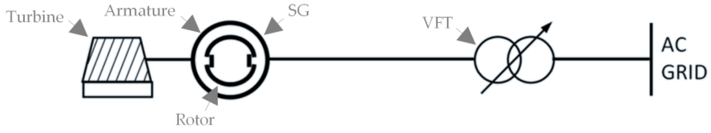
2.3. Variable Frequency Transformer
A variable frequency transformer (VFT) has been used in the interconnection of systems to control active and reactive power flow for a long time, in addition to being used to compensate for frequency fluctuations through a torque that is furnished by an external machine [
40,
41]. Nevertheless, this device has not been used to connect variable speed hydro generation synchronously to a system. Essentially, it is a wound rotor induction motor acting as a transformer, i.e., the stator is the primary transformer and the rotor is the secondary one [
41,
42].
Figure 3 presents a connection using the VFT. In this case, all of the generated power passes through the VFT.
A synchronous machine rotates at synchronous speed and, in order to obtain a rated frequency in its output, it is excited with a DC current. On the other hand, a regular transformer is a static machine. Thus, in order to have rated frequency in its output, rated frequency must be inserted directly into its input. Hence, it can be concluded that if the frequency of input and output are different, the machine must rotate at a given speed that is proportional to this difference in order to match primary and secondary frequencies [
40,
41].
The VFT is driven by a DC motor and the rotation speed of the VFT is proportional to the difference in frequencies. The power used to rotate the machine is inserted in the system and efficiency is about 98%. Nevertheless, all of the slip rings and brushes must be conveniently sized to afford all of the power generated [
42,
43].
This alternative has the advantage of maintaining the used synchronous generator along with its regular excitation system. Both active and reactive powers are normally controlled. Therefore, in a retrofit scenario, all of the system remains the same, except the installation of the VFT, which requires a large amount of space. The VFT can be installed for one machine or for the whole power plant. In general, it is manufactured at the rated power of 100 MW. This means that it can be connected to power plants with rated power less than 100 MW. However, different rated power can certainly be achieved.
2.4. Direct Current Transmission
The use of a High Voltage Direct Current transmission system (HVDC) is very popular to connect unsynchronized AC power systems [
44,
45], 50 Hz and 60 Hz power systems such as those used in Japan and in South America [
46,
47], long distance power transmissions [
48,
49], underwater transmission systems [
50], and variable frequency renewable generations [
51,
52].
Therefore, if the generator is connected through an HVDC to the power system, the speed it runs and the frequency of the voltage that it generates does not matter. The generated power is rectified and connected to the grid.
Figure 4 shows the synchronous generator connected to an HVDC system.
This is a practical solution for a retrofit scenario, mainly because the generation system remains almost the same [
53,
54]. Space must be provided only to accommodate the converter, which inherently consumes some reactive power with trivial synchronization. Power to feed auxiliary systems must also be provided. On the other hand, it has a straightforward application in hydropower plants connected to the system through a HVDC.
3. Francis Turbine Operating at Variable Head and Speed
There are several types of runners for hydropower plant application. Specifically, a turbine considers all of the mechanical components that surround the runner, including case, flow controllers, bearings, valves, draft tubes, and other components. The most common runners are Pelton, Francis, and Kaplan, whose names are a tribute to their inventors. Pelton runners are suitable for high head and small flow, while Kaplan runners are better for low head and high flow. The terms high and low heads are relative and depend fundamentally on the flow [
4,
5].
On the other hand, because of its geometry, the Francis runner type is the most flexible runner. It works well within the limits of the Pelton and Kaplan runners, as it can operate under high head and small flow, and at low head and high flow. A dimensionless quantity defined as specific speed (
) function of speed, flow, and head depicts such limits:
where n is the rotational speed (rpm), Q is the flow (m
3/s), and H is the net head (m).
In rated conditions of speed, head, and flow, a hydraulic machine may reach its maximum efficiency in energy conversion and a cavitation and vibration-free operation [
55,
56,
57,
58].
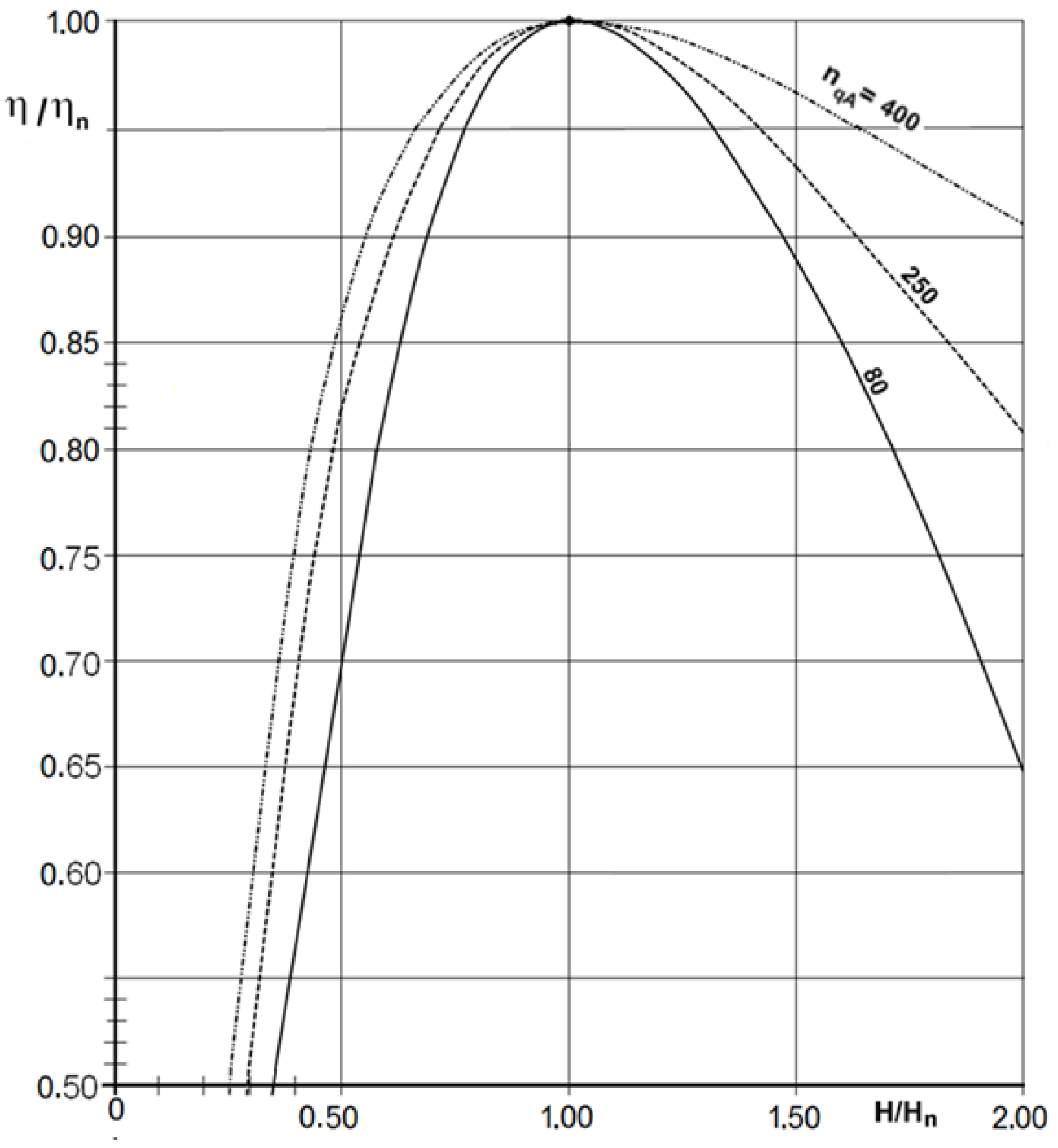
Figure 5 shows three types of Francis runners, namely slow, normal, and fast specific speed runners, which are suitable for high, average, and low heads, respectively, with specific rotation ranging from 70 to 400.
Thus, once designed for a specific rated condition, the Francis runner must work within very narrow application limits. The head and flow must be kept constant in order to achieve maximum energy conversion efficiency. While the Francis runner is known to allow a wide variation in its operating flow, changes in the head result in an extreme reduction of efficiency.
Figure 6 and
Figure 7 present the normalized efficiency curves of Francis runners for four different specific speeds as a function of the normalized flow and for the normalized head at constant rotational speed and head [
59,
60,
61].
It is common to present normalized quantities using their rated values as a basis. Therefore,
and
are the rated flow and head.
Figure 6 also shows the minimum normalized flow to limit a maximum of 10% reduction in the rated energy conversion efficiency.
Based on Equation (1), it can be seen that a head reduction could be compensated by speed reduction in order to achieve the design specific speed, while consequently recovering the rated efficiency. Nevertheless, a head reduction also conducts to a flow reduction in a proportion that depends on the runner design. This deserves a more detailed study.
Figure 8 depicts a cut in the Francis runner, wherein the mean flux line and main diameters of the turbine D (m), lengths L (m), diameters of the water flow path b (m), and angles, in several important sections—2, 4, and 5—are presented. The subscripts added to these quantities mean internal (i), mean (m), and external (e). The rotor has a relative speed and tangential velocity in relation to the stator, u (m/s).
The Euler equation relates head, speed, and flow to the dimensional quantities, as follows:
with
In these equations, a, b, and c are polynomial coefficients, S is the cross-section area (m2), and g is the gravitational constant (m/s2).
Considering an average flux line, a velocity triangle depicted in
Figure 9 can be obtained, where w is the mean relative speed (m/s), c
m is the meridional mean speed (m/s), c
u is the projection of the mean speed to the tangential direction (m/s), c is the mean absolute speed in the rotor entrance (m/s), β is the angle between the tangential velocity and the mean relative speed (degrees), and α is the angle between the tangential velocity and the mean absolute speed of the rotor entrance (degrees).
This diagram in
Figure 10 is drawn considering the rated point of operation and loading. If the machine is loaded under or above the rated point, a chock component appears, which reduces the efficiency of the turbine. The hydro turbine is designed for a rated rotational speed, head, and flow, resulting in a specific speed, as stated in (1). Therefore, for each operational H, values of n and Q must be calculated in order to satisfy the Euler equation in which a third-degree equation is reached (6):
where
is the rated turbine efficiency and
(m) is the average turbine input diameter.
As an example, a turbine with rated flow values of 12.536 m
3/s, head 60 m, speed 360 rpm, efficiency 0.948, and an input diameter of 1.280 m, operates at a 10% increase in the head. Therefore, on applying the aforementioned equations, the turbine has to operate at a speed of 377.6 rpm. The resulting velocity triangle is depicted in
Figure 8. The increase in power was 15.4% in the flow and speed was 4.9%, thus maintaining the rated efficiency.
It should be noted that the aperture of the gates must be such that is necessary in order to obtain the calculated speed. The speed is calculated in accordance with the available head and by the electrical generator, as it is directly defined by the supplied load.
4. Experimental Method
The hydropower plants are designed to have maximum efficiency at a rated head and flow. Nonetheless, it is recognized that both of these quantities vary with time. While flow variation is certainly manageable, head variations are harmful and undesirable. Therefore, varying speed of the generating unit is proposed in order to recover the speed specific to the rated conditions and to maintain maximum efficiency of the turbine.
The following sections deal with the characterization of a test setup that was specially developed to test the behavior of the unit under head variations. Efficiency tests are applied and results are presented.
4.1. Experimental Testing Setup
In order to test variable speed generation connected to the grid, a test bench was developed, as depicted in
Figure 11. The length dimensions are in millimeters (mm), unless described otherwise. In this bench, water is pumped into a reservoir that enables the operation in two different upstream levels. The flow passes through the penstock to the hydraulic turbine before going to the downstream reservoir. After passing through a convenient rectangular weir, the water goes to a storage reservoir, and is then pumped again to establish the upper level.
There is a movable diverter inside the tank, which allows the operation with two different upstream levels, named NMI and NMII. As long as the downstream level is constant (NJ), the efficiency of the hydraulic turbine with the Francis runner (THF) can be obtained and compared with the two different gross heads at constant and variable operational speeds.
The rated quantities of the hydraulic turbine are shown in
Table 1. The water flow (Q) through the turbine is measured as the average of two different methods, described and referred to in main hydraulic machinery testing standards [
62,
63]. This procedure guarantees redundancy in this important and difficult measurement. In the first method, water flow is calculated as a function of the measured spill height over the weir; the main dimensional characteristics are described in
Table 2 [
62].
The second technique for flow measurement is the Winter-Kennedy method. This approach is based on the measurement of differential pressure in the turbine casing, which appears due to water streams velocity differences in both the inner and outer part of the case. Eventually, the flow is proportional to the square root of this pressure difference.
The hydraulic turbine converts hydraulic power to mechanical power, which is a function of the torque and rotational speed in the coupling shaft. The electric generator converts the mechanical power into electric power. The generator is conveniently designed to have a minimum mechanical losse, including a special magnetic winding to reduce the pressure over the bearings and independent external ventilation. The generated electric power, which is of variable frequency, is transferred to the constant frequency system using a back-to-back converter.
A picture of the laboratory setup is showed in
Figure 12.
Figure 12a shows the upstream tank, turbine spiral casing, coupling, and generator.
Figure 12b shows the hydraulic turbine draft tube, downstream tank, and the converter from behind.
The quality of the optimal behavior of a hydropower unit is measured by its efficiency of energy conversion. Whilst head and flow variations mean nothing to the electrical generator as it is only concerned with the power delivered in the connecting mechanical shaft [
63], the hydraulic turbine has its efficiency closely attached to these parameters and governed by its hill chart.
Therefore, there are three involved efficiencies: the efficiency of the hydraulic turbine (
), the efficiency of the electric generator (
), and the efficiency of the power converter (
), all of which are functions of the hydraulic power (
), turbine power (
), electric power (
), and grid power (
). The efficiencies are calculated using Equations (7)–(9). While the efficiencies are per unit values, all of the powers are given in kW.
Both electric power in the generator terminals and the grid power in the converter output are straight and measured directly using special watt meters. The hydraulic power and turbine power result from calculation using measured quantities. The employed sensors to measure these quantities, and their respective accuracy class, are depicted in
Table 3. The accuracy class is the maximum expected error in a measurement, and normally is a percentage of the sensor full scale.
Hydraulic power is a function of the available head H (m), flow Q (m
3/s), water density ρ (kg/m
3), and local gravity acceleration g (m/s
2), as described in (10). The turbine power is the power available in the mechanical shaft. It is a function of the torque M (Nm) and speed n (rpm), calculated using (11):
The rectangular weir flow equation (
), function of the height of the water spill over the rectangular wear, and the flow using Winter-Kennedy technique (
) are given by the following models:
The value of the flow at the turbine is the average of both measurements
and
.
and
are constants obtained from calibrations [
62], while
(m) and
are the level over the weir and the differential pressure measured in turbine spiral casing.
Referring to the dimensions and measurements described in
Figure 11, the water head is:
where
is the input static pressure (m),
are the areas of the cross sections
and
(m
2),
are heights in points 1, 2, and
(m).
The density is a function of the water temperature
(°C):
The final efficiency calculation accuracy is a function of the accuracy of each of the used sensors, partial derivatives calculations, the number of measurements in each point (standard deviation), and of the value of the measured quantity itself. The final efficiency accuracy is described in main hydraulic machinery testing standards [
64,
65].
4.2. Efficiency Testing Measurements
The developed test rig was applied to assess the turbine goodness behavior operating at two different heads with constant and rated speed, along with variable speed. The main quantity of appreciation was the efficiency of energy conversion, among others, such as used water flow, which employs previous mathematical statements.
The first test was developed at a constant rated head of the turbine at 2.95 m and rated speed. Load variation was applied and the flow varied accordingly.
Table 4 presents the main variables resultant from this test. The measured efficiency calculated using Equation (7) was kept classified by using the normalized results (calculated by dividing the measured values obtained in tests by the maximum measured value).
The second test was performed with a head reduction, and constant and rated speed. The testing head was approximately 2.20 m, representing a reduction of about 25%. The main results are described in
Table 5. The presented efficiency results are normalized, taking maximum efficiency in the test at rated conditions as a reference.
It is clear that there is a reduction in efficiency of the hydraulic turbine. A reduction of about 20% can be seen in maximum normalized efficiency, which can be larger in other loads. It can also be seen that the flow has a reduction, as it directly depends on the head. As a result, there is a reduction on the delivered power, as both the head and flow are reduced.
A third test was conducted at the reduced head of 2.2 m. In this new test, speed is also reduced according to Equation (6). For a head of 2.2 m, speed should be 386 rpm. However, during the tests, a value of around 386 rpm was achieved. The obtained hydraulic turbine, along with the conditions of the test, is depicted in
Table 6.
Figure 13 presents the graphical results of this test in comparison to the obtained results of the two previous tests. Curve (a) was obtained with rated head and speed, curve (b) is the efficiency curve for rated speed and low head, and curve (c) represents the efficiency at a lower head and lower speed.
Despite the flow and power reduction, as the head is smaller than the rated head, an increase of normalized efficiency can be observed, and maximum efficiency approximately reaches the maximum efficiency at rated conditions. It can be seen that there was an increase of about 20% in the normalized efficiency, thus enhancing the advantages of operating at a low speed when a reduction in the head is noticed.
5. Application to Furnas Hydropower Plant
Variable speed generation application was evaluated for the Furnas hydropower plant, considering its gross head variation history. The Furnas power plant is located in the southern part of the state of Minas Gerais, Brazil, as shown in
Figure 14a, obtained from [
66]. The power plant has a large reservoir, with a surface area of 1440 km
2 at the maximum upstream level and a perimeter of about 3500 km, which is equal to almost half of the Brazilian coastline. The total volume of water is 22,590 km
3 with a storage volume of 17,217 km
3. This power plant has an installed power of 1280 MVA and a rated head of 98.83 m [
67].
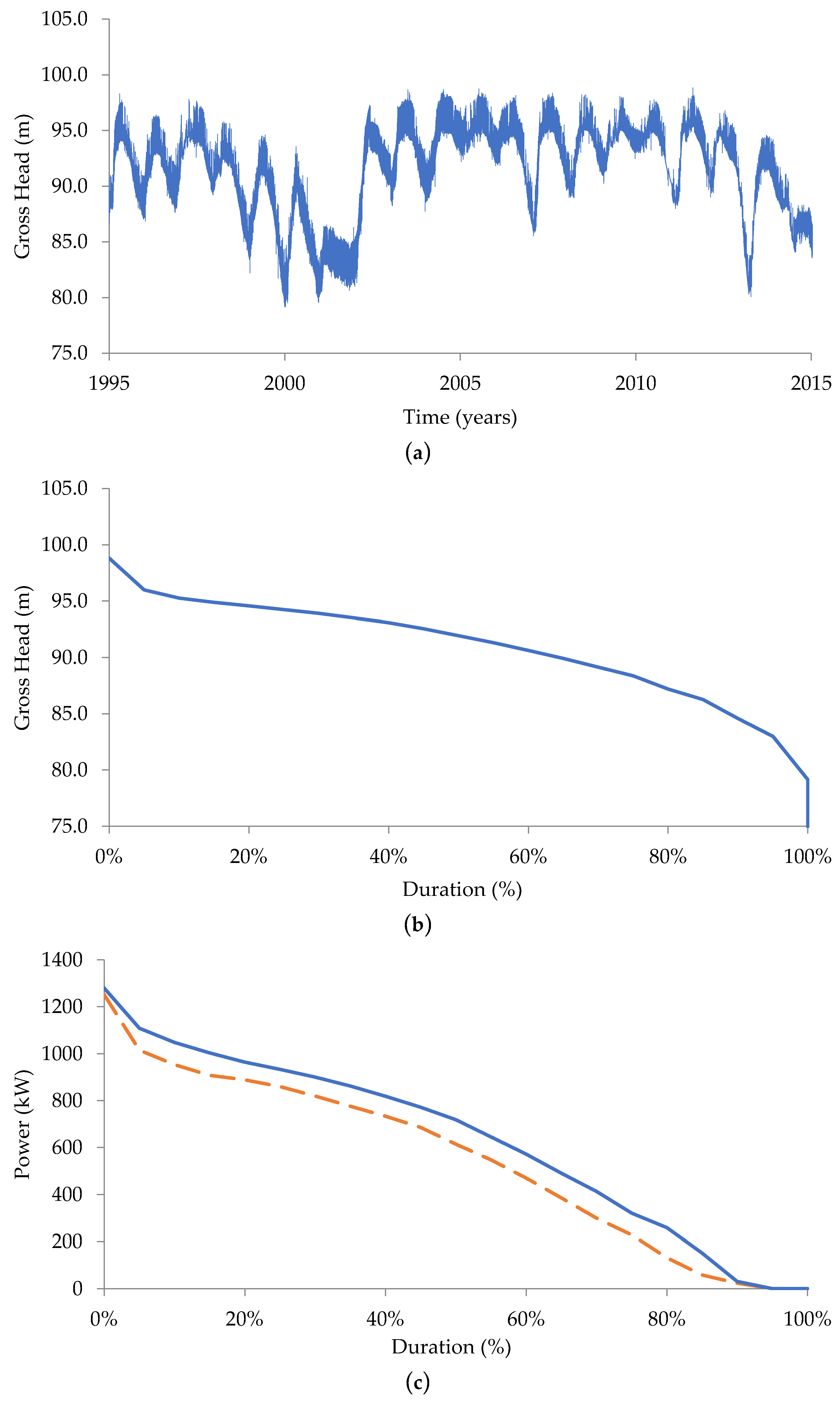
Figure 15a presents the gross head variation over time, recorded from 1995 to 2015. The gross head can be as low as 79 m, which means a gross head variation of about 20% in the worst-case scenario, and reflecting the total use of the reservoir storage volume.
The hydro turbine suffers from such head variations, which lead to an increase in losses, appearance of vortex, cavitation, and vibration, which result in premature wear and undesired efficiency reduction. While
Figure 15a shows the gross head variation over time,
Figure 15b presents the resultant gross head duration curve.
The concept of a duration curve is used in many applications, and shows the probability of this value to be reached or overcome for each value. For instance, a gross head of 83 m is overcome more than 95% of the time, while a head of 96 m is reached only 5% of the entire time. The advantage of using a duration curve resides in the use of few experiments, rather than the entire raw curve of time stamped data, without losing the most important information.
It is well known that there are many advantages of operating at a constant rated head. Not only will the hydraulic machine operate at optimal conditions, but the generated power will additionally be at its maximum, as it is directly proportional to the operating head. The higher the head, the larger the generated power will be.
However, the Furnas power plant plays a very important role not only in the cascade of the Grande River basin, but also in the whole Brazilian hydraulic power generation system, as well as for navigation purposes. Its enormous reservoir is capable of regularizing all water flow in the Grande River basin. This water passes through important and powerful hydropower plants along the cascade before ending up in the Itaipu hydropower plant, which is one of the largest power plants in Brazil.
Figure 14b illustrates the location of the Furnas power plant in a partial Brazilian hydropower system chart.
Several scientific studies show the dependence of the optimal operation of the entire Brazilian power system with the Furnas hydropower plant [
68,
69]. Therefore, it becomes natural to affirm that the storage volume in the Furnas reservoir will always be requested in order to regulate water flow, not only in the Rio Grande basin, but also along the entire cascade, all the way to the Itaipu Hydropower plant, leading to variations in the gross head of the power plant. Variations in the gross head of the power plant will constantly be seen and operations with variable speed will allow the Furnas power plant to operate at its best efficiency.
The generating units of Furnas hydropower plant operate at constant speed, leading to turbine efficiency reduction. Both the theoretical analysis and the laboratory tests show that running the hydro turbine at a reduced speed could recover its efficiency. The amount of energy recovered is proportional to the recovered efficiency, which is a function of the operating head versus the rated head.
Figure 15c depicts the duration curve of the power generated with the gross head variation at constant speed and, using the theory presented in this paper, the power that could be generated if the speed could vary.
Regarding
Figure 15c, the lower dashed curve shows the actual generated power, while the upper continuous curve presents the power that could be generated if the generating units could operate at a variable speed. The variable speed operation allows a bigger generation, not only because of the increase in turbine efficiency, but also because the flow rate in the machines also increases, as has been verified by laboratory tests.
The area under a power versus time curve results in energy. The same principle can be seen with the duration curve. The remarkable difference is that instead of having the abscissa axis as a time unit, such as hours or days, the duration curve has its abscissa axis in percentile. Therefore, instead of having energy as a multiple of watthours, the area under the curve will be energy in an average power unit. The energy in watthour is the energy in average power times the base of the time. The base of the time normally used is the number of hours in a year, i.e., 8760 h. Therefore, the result of the area under the curve must be multiplied by 8760 in order to show energy in watthour multiples.
Applying this technique to the presented curves results in an average power of 551.4 MW for the operation at constant speed and an average power of 632.7 MW for the operation at variable speed, thus confirming the increase in generation with the variable speed operation.
The difference of both results is additional generation of 712.6 GWh, which is sufficient to cover the expenses in updating the generation system to operate with variable speed. Other economic benefits of the application of variable speed are the reduction of machine stopped time and reduction of expenses with maintenance of turbine and bearings, which are proportional to the diminution of cavitation and associated vibration.
6. Conclusions
As a consequence of climate change, hydro cascade operation, and inflow reduction, the upstream level of the reservoirs of some hydropower plants has decreased. This has further caused a reduction in the resulting water head and energy conversion of hydro turbines. Through theoretical analysis and laboratorial application, this paper shows that the variable speed operation of the units of a hydropower plant can recover the efficiency of rated values. The operation at variable speed results in a variable frequency of the generated voltage. Therefore, this paper also presents some alternatives to connecting the modified hydropower plant to a constant frequency grid. The theory of operating Francis runners at variable speed was presented and a suitable equation to determine the operating speed necessary to recover the hydro turbine efficiency to rated levels was developed and presented. A special laboratory setup was constructed to verify the functionality of the proposed theory. In short, three tests were conducted at two different upstream levels. The first test was performed at rated water head and speed, achieving a rated efficiency curve. In the second test at reduced water head and rated speed, a capital reduction of the energy conversion efficiency was verified, as long as the hydro turbine was in an unfavorable condition. A third test was attempted at a reduced head and reduced speed, as defined by the developed equation, and the recovery of the hydro turbine efficiency up to rated levels was verified, confirming the developed theory. Therefore, reduction of the operating speed when the upstream level is less than rated and conducting to the reduced water head demonstrated energy benefits, as was theoretically expected. The energy benefit of operating at variable speeds was determined for the Furnas hydropower plant, which is known to have a history of upstream level variation. The variable speed operation increased the average power generation by about 15% per year with proportional increase in power plant revenues. This study did not determine the costs of turning a regular hydropower plant into a variable speed capable hydropower plant, as that requires additional equipment and space. In addition, the study did not determine the supplementary benefits of operating at a lower speed, such as gains with maintenance, as the hydro turbine operates free of cavitation and vibration, which translates as longevity of mechanical parts. These aspects will be studied in future research.
Author Contributions
Conceptualization, E.B., Z.d.S., and A.V.; methodology, E.B., Z.d.S., and A.V.; software, E.B., R.B., and J.B.J.; validation, E.B., A.V. and J.B.J.; formal analysis, E.B., Z.d.S., and A.V.; investigation, E.B., Z.d.S., and A.V.; resources, L.P. and R.S.; data curation, X.X.; writing—original draft preparation, E.B., L.P. and H.V.-N.; writing—review and editing, E.B., L.P. and H.V.-N.; visualization, R.B., and J.B.J.; supervision, E.B., A.V., and Â.R.; project administration, A.V.; funding acquisition, L.P. and R.S.
Funding
This research was partially funded by ANEEL R&D program.
Acknowledgments
The authors would like to thank FAPEMIG, CNPq, CAPES, INERGE and FURNAS for their support.
Conflicts of Interest
The authors declare no conflict of interest.
References
- Kerkman, R.J.; Lipo, T.A.; Newman, W.G.; Thirkell, J.E. An inquiry into adjustable speed operation of a pumped hydro plant. Part 1—Machine design performance. IEEE Trans. Power Appar. Syst. 1980, 99, 1828–1837. [Google Scholar] [CrossRef]
- Barros, J.G.C.; Saidel, M.A.; Ingram, L.; Westphalen, M. Adjustable speed operation of hydroelectric turbine generators. Electra 1996, 167, 17–36. [Google Scholar]
- Fraile-Ardanuy, J.; Wilhelmi, J.R.; Fraile-Mora, J.J.; Perez, J.I. Variable-Speed Hydro Generation: Operational Aspects and Control. IEEE Trans. Energy Convers. 2006, 21, 569–574. [Google Scholar] [CrossRef]
- Souza, Z.; Santos, A.H.M.; Bortoni, E.C. Hidro Power Plants—Studies for Implantation, 3rd ed.; Interciencia: Rio de Janeiro, Brazil, 2018. (In Portuguese) [Google Scholar]
- Macintyre, A.J. Hydraulic Machines; Guanabara: Rio de Janeiro, Brazil, 1983. [Google Scholar]
- Roy, U.; Majumder, M. Impact of climate change on small scale hydro-turbine selections. In Springer Briefs in Energy; Springer: Berlin, Gremany, 2016. [Google Scholar]
- Santhosh, A.; Farid, A.M.; Youcef-Toumic, K. The impact of storage facility capacity and ramping capabilities on the supply side economic dispatch of the energy-water nexus. Energy 2014, 66, 363–377. [Google Scholar] [CrossRef]
- Gaudard, L.; Gilli, M.; Romerio, F. Climate Change Impacts on Hydropower Management. Water Res. Manag. 2013, 27, 5143–5156. [Google Scholar] [CrossRef] [Green Version]
- Schaeffer, R.; Szklo, A.S.; Lucena, A.F.P.; Borba, B.S.M.C.; Nogueira, L.P.P.; Fleming, F.P.; Troccoli, A.; Harrison, M.; Boulahya, M.S. Energy sector vulnerability to climate change: A review. Energy 2012, 38, 1–12. [Google Scholar] [CrossRef]
- Scott, C.A.; Pierce, S.A.; Pasqualetti, M.J.; Jones, A.L.; Montz, B.E.; Hoover, J.H. Policy and institutional dimensions of the water-energy nexus. Energy Policy 2011, 39, 6622–6630. [Google Scholar] [CrossRef]
- Queiroz, A.R. Stochastic hydro-thermal scheduling optimization: An overview. Renew. Sustain. Energy Rev. 2016, 62, 382–395. [Google Scholar] [CrossRef]
- Fernandes, G.; Gomes, L.L.; Brandão, L.E.T. A risk-hedging tool for hydro power plants. Renew. Sustain. Energy Rev. 2018, 90, 370–378. [Google Scholar] [CrossRef]
- Singh, K.; Singal, S.K. Operation of hydro power plants-a review. Renew. Sustain. Energy Rev. 2017, 69, 610–619. [Google Scholar] [CrossRef]
- Valavi, M.; Nysveen, A. Variable-Speed Operation of Hydropower Plants: A look at the past, present, and future. IEEE Ind. Appl. Mag. 2018, 24, 18–27. [Google Scholar] [CrossRef]
- Borkowski, D. Analytical Model of Small Hydropower Plant Working at Variable Speed. IEEE Trans. Energy Convers. 2018, 33, 1886–1894. [Google Scholar] [CrossRef]
- Pérez-Díaz, J.I.; Chazarra, M.; García-González, J.; Cavazzini, G.; Stoppato, A. Trends and challenges in the operation of pumped-storage hydropower plants. Renew. Sustain. Energy Rev. 2015, 44, 767–784. [Google Scholar] [CrossRef]
- Sedaghat, A.; Hassanzadeh, A.; Jamali, J.; Mostafaeipour, A.; Chene, W. Determination of rated wind speed for maximum annual energy production of variable speed wind turbines. Appl. Energy 2017, 205, 781–789. [Google Scholar] [CrossRef]
- Liu, Y.; Wang, Z.; Xiong, L.; Wang, J.; Jiang, X.; Bai, G.; Li, R.; Liu, S. DFIG wind turbine sliding mode control with exponential reaching law under variable wind speed. Electr. Power Energy Syst. 2018, 96, 253–260. [Google Scholar] [CrossRef]
- Fairley, P. A Renaissance for Pumped Hydro Storage. IEEE Spectr. 2015, 52, 9–10. [Google Scholar] [CrossRef]
- Rehman, S.; Al-Hadhrami, L.M.; Alam, M.M. Pumped hydro energy storage system: A technological review. Renew. Sustain. Energy Rev. 2015, 44, 586–598. [Google Scholar] [CrossRef]
- Schmidt, J.; Kemmetmüller, W.; Kugi, A. Modeling and static optimization of a variable speed pumped storage power plant. Renew. Energy 2017, 111, 38–51. [Google Scholar] [CrossRef]
- Mohanpurkara, M.; Ouroua, A.; Hovsapian, R.; Luo, Y.; Singh, M.; Muljadi, E.; Gevorgian, V.; Donalek, P. Real-time co-simulation of adjustable-speed pumped storage hydro for transient stability analysis. Electr. Power Syst. Res. 2018, 154, 276–286. [Google Scholar] [CrossRef]
- Costa, J.C.; Bortoni, E.C.; Vieira, P.A.V.; Faria, V.A.D. Energy system planning considering renewables and pumped-storage power plants. Int. J. Smart Grid Sustain. Energy Technol. 2017, 1, 32–38. [Google Scholar]
- Inage, S. The role of large-scale energy storage under high shares of renewable energy. Wires Energy Environ. 2015, 4, 115–132. [Google Scholar] [CrossRef]
- Bessa, R.; Moreira, C.; Silva, B.; Filipe, J.; Fulgêncio, N. Role of pump hydro in electric power systems. J. Phys. Conf. Ser. 2017, 813, 012002. [Google Scholar] [CrossRef] [Green Version]
- Louvet, R.; Neto, A.; Billet, L.; Passelergue, J.C. Smart dispatch of variable-speed Pump Storage Plants to facilitate the insertion of intermittent generation. In Proceedings of the Cigré Session 2016, Paris, France, 21–26 August 2016. [Google Scholar]
- Hozouri, M.A.; Abbaspour, A.; Fotuhi-Firuzabad, M.; Moeini-Aghtaie, M. On the use of pumped storage for wind energy maximization in transmission-constrained power systems. IEEE Trans. Power Syst. 2015, 30, 1017–1025. [Google Scholar] [CrossRef]
- Gomes, E.P.; Bajay, S.V. Brazilian hydroelectric rehabilitation potential and viability. Am. J. Hydro Power Water Environ. Syst. 1 2014, 1, 20–24. [Google Scholar] [CrossRef]
- Vargas-Serrano, A.; Hamann, A.; Hedtke, S.; Franck, C.M.; Hug, G. Economic benefit analysis of retrofitting a fixed-speed pumped storage hydropower plant with an adjustable-speed machine. In Proceedings of the IEEE Power Tech, Manchester, UK, 18–22 June 2017. [Google Scholar]
- Rahi, O.P.; Chandel, A.K. Refurbishment and uprating of hydro power plants—A literature. Renew. Sustain. Energy Rev. 2015, 48, 726–737. [Google Scholar] [CrossRef]
- Kouro, S.; Rodriguez, J.; Wu, B.; Bernet, S.; Perez, M. Powering the future of industry: High-power adjustable speed drive topologies. IEEE Ind. Appl. Mag. 2012, 18, 26–39. [Google Scholar] [CrossRef]
- Pannatier, Y.; Kawkabani, B.; Nicolet, C.; Simond, J.J.; Schwery, A.; Allenbach, P. Investigation of control strategies for variable-speed pump-turbine units by using a simplified model of the converters. IEEE Trans. Ind. Electron. 2010, 57, 3039–3049. [Google Scholar] [CrossRef]
- Padoan, A.C.P., Jr.; Kawkabani, B.; Schwery, A.; Ramirez, C.; Nicolet, C.; Simond, J.J.; Avellan, F. Dynamical behavior comparison between variable speed and synchronous machines with PSS. IEEE Trans. Power Syst. 2010, 25, 1555–1565. [Google Scholar]
- Cárdenas, R.; Espina, E.; Clare, J.; Wheeler, P. Self-Tuning Resonant Control of a Seven-Leg Back-to-Back Converter for Interfacing Variable-Speed Generators to Four-Wire Loads. IEEE Trans. Ind. Elect. 2015, 62, 4618–4629. [Google Scholar] [CrossRef]
- Miranbeigi, M.; Iman-Eini, H.; Asoodar, M. A new switching strategy for transformer-less back-to-back cascaded H-bridge multilevel converter. IET Power Electron. 2014, 7, 1868–1877. [Google Scholar] [CrossRef]
- Li, S. Power Flow Modeling to Doubly-Fed Induction Generators (DFIGs) Under Power Regulation. IEEE Trans. Power Syst. 2013, 28, 3292–3301. [Google Scholar] [CrossRef]
- Zhang, Y.; Ooi, B.T. Stand-Alone Doubly-Fed Induction Generators (DFIGs) With Autonomous Frequency Control. IEEE Trans. Power Deliv. 2013, 28, 752–760. [Google Scholar] [CrossRef]
- Lung, J.K.; Lu, Y.; Hung, W.L.; Kao, W.S. Modeling and Dynamic Simulations of Doubly Fed Adjustable-Speed Pumped Storage Units. IEEE Trans. Energy Convers. 2007, 22, 250–258. [Google Scholar] [CrossRef]
- Bocquel, A.; Janning, J. Analysis of a 300 MW variable speed drive for pump-storage plant applications. In Proceedings of the European Conference on Power Electronics and Applications, Dresden, Germany, 11–14 September 2005. [Google Scholar]
- Ambati, B.B.; Khadkikar, V. Variable frequency transformer configuration for decoupled active-reactive powers transfer control. IEEE Trans. Energy Convers. 2016, 31, 906–914. [Google Scholar] [CrossRef]
- Ambati, B.B.; Kanjiya, P.; Khadkikar, V.; el Moursi, M.S.; Kirtley, J.L., Jr. A hierarchical control strategy sith fault ride-through capability for variable frequency transformer. IEEE Trans. Energy Convers. 2015, 30, 132–141. [Google Scholar] [CrossRef]
- Merkhouf, A.; Doyon, P.; Upadhyay, S. Variable frequency transformer—Concept and electromagnetic design evaluation. IEEE Trans. Energy Convers. 2008, 23, 989–996. [Google Scholar] [CrossRef]
- Bakhsh, F.I.; Khatod, D.K. A new synchronous generator based wind energy conversion system feeding an isolated load through variable frequency transformer. Renew. Energy 2016, 86, 106–116. [Google Scholar] [CrossRef]
- Hingorani, N.G. High-Voltage DC Transmission: A power electronics workhorse. IEEE Spectr. 1996, 33, 63–72. [Google Scholar] [CrossRef]
- Guarnieri, M. The alternating evolution of DC power transmission. IEEE Ind. Electron. Mag. 2013, 7, 60–63. [Google Scholar] [CrossRef]
- Velasco, D.; Trujillo, C.L.; Peña, R.A. Power transmission in direct current. Future expectations for Colombia. Renew. Sustain. Energy Rev. 2011, 15, 759–765. [Google Scholar] [CrossRef]
- Sousa, T.; Santos, M.L.D.; Jardini, J.A.; Casolari, R.P.; Nicola, G.L.C. An evaluation of the HVDC and HVAC transmission economic. In Proceedings of the IEEE/PES Transmission and Distribution, Montevideo, Uruguay, 3–5 September 2012. [Google Scholar]
- Kalair, A.; Abas, N.; Khan, N. Comparative study of HVAC and HVDC transmission systems. Renew. Sustain. Energy Rev. 2016, 59, 1653–1675. [Google Scholar] [CrossRef]
- Benasla, M.; Allaoui, T.; Brahami, M.; Denaï, M.; Sood, V.K. HVDC links between North Africa and Europe: Impacts and benefits on the dynamic performance of the European system. Renew. Sustain. Energy Rev. 2017, 82, 3981–3991. [Google Scholar] [CrossRef]
- Liu, L.; Liu, C. VSCs-HVDC may improve the Electrical Grid Architecture in future world. Renew. Sustain. Energy Rev. 2016, 62, 1162–1170. [Google Scholar] [CrossRef]
- Guimarães, R.P.; Miller, M.D. Brazilian transmission system: A race for the future. In Proceedings of the Electrical Transmission and Substation Structures Conference, Columbus, OH, USA, 4–8 November 2012. [Google Scholar]
- Pierri, E.; Binder, O.; Hemdan, N.G.A.; Kurrat, M. Challenges and opportunities for a European HVDC grid. Renew. Sustain. Energy Rev. 2017, 70, 427–456. [Google Scholar] [CrossRef]
- Naidu, M.; Mathur, R.M. Evaluation of unit connected, variable speed, hydropower station for HVDC power transmission. IEEE Trans. Power Syst. 1989, 4, 668–676. [Google Scholar] [CrossRef]
- Arrillaga, J.; Sankar, S.; Arnold, C.P.; Watson, N.R. Characteristics of unit-connected HVDC generator-convertors operating at variable speeds. IEE Proc. C Gener. Trans. Distrib. 1992, 139, 295–299. [Google Scholar] [CrossRef]
- Heckelsmueller, G.P. Application of variable speed operation on Francis turbines. Ing. E Investig. 2015, 35, 12–16. [Google Scholar] [CrossRef]
- Trivedi, C.; Agnalt, E.; Dahlhaug, O.G. Investigations of unsteady pressure loading in a Francis turbine during variable-speed operation. Renew. Energy 2017, 113, 397–410. [Google Scholar] [CrossRef]
- Working Group on Prime Mover and Energy Supply Models for System Dynamic Performance Studies. Hydraulic turbine and turbine control models for system dynamic studies. IEEE Trans. Power Syst. 1992, 7, 167–179. [Google Scholar] [CrossRef]
- Cavazzini, G.; Houdeline, J.B.; Pavesi, G.; Teller, O.; Ardizzon, G. Unstable behaviour of pump-turbines and its effects on power regulation capacity of pumped-hydro energy storage plants. Renew. Sustain. Energy Rev. 2018, 94, 399–409. [Google Scholar] [CrossRef]
- Borkowski, D.; Wegiel, T. Small Hydropower Plant with Integrated Turbine-Generators Working at Variable Speed. IEEE Trans. Energy Convers. 2013, 28, 452–459. [Google Scholar] [CrossRef]
- Borkowski, D. Maximum efficiency point tracking (MEPT) for variable speed small hydropower plant with neural network based estimation of turbine discharge. IEEE Trans. Energy Convers. 2017, 32, 1090–1098. [Google Scholar] [CrossRef]
- Zhang, J.; Leontidis, V.; Dazin, A.; Tounzi, A.; Delarue, P.; Caignaert, G.; Piriou, F.; Libaux, A. Canal locks variable speed hydropower turbine design and control. IET Renew. Power Gener. 2018, 12, 1698–1707. [Google Scholar] [CrossRef]
- Bortoni, E.C.; Rocha, M.S.; Rodrigues, M.A.S.; Laurindo, B.C.S. Calibration of weirs using unsteady flow. Flow Meas. Instrum. 2017, 57, 73–77. [Google Scholar] [CrossRef]
- Garcia, F.J.; Uemori, M.K.I.; Echeverria, J.J.R.; Bortoni, E.C. Design requirements of generators applied to low-head hydro power plants. IEEE Trans. Energy Convers. 2015, 28, 1630–1638. [Google Scholar] [CrossRef]
- ASME. Hydraulic Turbines and Pump-Turbines; ASME PTC 18-2011; The American Society of Mechanical Engineers: New York, NY, USA, 2011; p. 94. [Google Scholar]
- IEC. Field Acceptance Tests to Determine the Hydraulic Performance of Hydraulic Turbines, Storage Pumps and Pump-Turbines; IEC 60041:1991; IEC: Geneva, Switzerland, 1991; 419p. [Google Scholar]
- Dias, V.S.; Luz, M.P.; Medero, G.M.; Nascimento, D.T.F.; Oliveira, W.N.; Meirelles, L.R.O. Historical Streamflow Series Analysis Applied to Furnas HPP Reservoir Watershed Using the SWAT Model. Water 2018, 10, 458. [Google Scholar] [CrossRef]
- FURNAS. Generating facts: Furnas Hydropower Plant. Available online: http://www.furnas.com.br/hotsites/sistemafurnas/usina_hidr_furnas.asp (accessed on 1 January 2019). (In Portuguese).
- Almeida, R.A.; Santos, A.H.M.; Bortoni, E.C.; Cabral, R.S. Evaluation of the increase of power generation in Brazilian hydro basins. In Proceedings of the IX ELPAH—Encuentro Latinoamericano y del Caribe Sobre Pequeños Aprovechamientos Hidroenergeticos, Neuquén, Argentina, 28 May 2001. (In Portuguese). [Google Scholar]
- Almeida, R.A.; Félix, B.F. Conti-Varlet application to evaluate the energy impact of cascade hydropower plants due to upstream reservoir depletion (In Portuguese). In Proceedings of the XXI Brazilian Symposium of Hydro Resources, Brasília, Brazil, 22 November 2015. [Google Scholar]
Figure 1.
Use of a back-to-back frequency converter.
Figure 1.
Use of a back-to-back frequency converter.
Figure 2.
Use of a double-fed asynchronous machine.
Figure 2.
Use of a double-fed asynchronous machine.
Figure 3.
Connection through a VFT.
Figure 3.
Connection through a VFT.
Figure 4.
Connection to a HVDC system.
Figure 4.
Connection to a HVDC system.
Figure 5.
Low specific speed (a), normal specific speed (b), and high specific speed (c) Francis runners suitable for high, average, and low heads, respectively.
Figure 5.
Low specific speed (a), normal specific speed (b), and high specific speed (c) Francis runners suitable for high, average, and low heads, respectively.
Figure 6.
Efficiency curves of Francis runners as a function of normalized flow.
Figure 6.
Efficiency curves of Francis runners as a function of normalized flow.
Figure 7.
Efficiency curves of Francis runners as a function of the normalized head.
Figure 7.
Efficiency curves of Francis runners as a function of the normalized head.
Figure 8.
Average flux line and main dimensions and angles for the reaction turbines.
Figure 8.
Average flux line and main dimensions and angles for the reaction turbines.
Figure 9.
Velocity triangle.
Figure 9.
Velocity triangle.
Figure 10.
Resulting velocity triangle.
Figure 10.
Resulting velocity triangle.
Figure 11.
Experimental laboratory installation layout.
Figure 11.
Experimental laboratory installation layout.
Figure 12.
Constructed laboratory installation setup.
Figure 12.
Constructed laboratory installation setup.
Figure 13.
Behavior of the hydraulic turbine at two different heads, constant and variable speed.
Figure 13.
Behavior of the hydraulic turbine at two different heads, constant and variable speed.
Figure 14.
Location map of the Furnas Hydropower plant [
66] (
a), and Grande River cascade and partial Brazilian hydropower system (
b).
Figure 14.
Location map of the Furnas Hydropower plant [
66] (
a), and Grande River cascade and partial Brazilian hydropower system (
b).
Figure 15.
Operation characteristics of the Furnas hydro power plant. Gross head variation over the years (a), gross head duration curve (b), and generated power duration curve (c).
Figure 15.
Operation characteristics of the Furnas hydro power plant. Gross head variation over the years (a), gross head duration curve (b), and generated power duration curve (c).
Table 1.
Hydro turbine rated quantities.
Table 1.
Hydro turbine rated quantities.
| Q (m3/s) | H (m) | n (rpm) | nqA |
|---|
| 0.156 | 4.16 | 450 | 183 |
Table 2.
Design characteristics of the rectangular weir.
Table 2.
Design characteristics of the rectangular weir.
| Quantity | Value | Unit |
|---|
| Weir width | 0.600 | (m) |
| Width of the channel | 1.000 | (m) |
| Gravity acceleration | 9.785 | (m/s2) |
| Distance from bottom to floor | 0.750 | (m) |
Table 3.
Main characteristics of the sensors.
Table 3.
Main characteristics of the sensors.
| Sensor | Symbol | Range | Accuracy Class |
|---|
| Static pressure transmitter | | 0–5 m | 0.02% |
| Differential pressure transmitter | | 0–1 m | 0.1% |
| Static pressure transmitter | | 0–1 m | 0.1% |
| Static pressure transmitter | | 0–1 m | 0.1% |
| Water temperature | | 0–100 °C | 0.1% |
| Rotating speed meter | - | 0–1000 rpm | 1 rpm |
| Torque transducer | - | 0–50 Nm | 0.1% |
| Generator power meter | | 0–20 kW | 0.5% |
| System power meter | | 0–20 kW | 0.5% |
Table 4.
Efficiency measurement at rated head and rated speed.
Table 4.
Efficiency measurement at rated head and rated speed.
| Head (m) | Flow (m3/s) | Speed (rpm) | Turbine Efficiency (%) |
|---|
| 2.948 | 0.158 | 450 | 68.33 |
| 2.954 | 0.157 | 450 | 80.88 |
| 2.952 | 0.152 | 450 | 89.24 |
| 2.951 | 0.149 | 450 | 95.48 |
| 2.952 | 0.139 | 450 | 100.0 |
| 2.950 | 0.136 | 450 | 94.74 |
Table 5.
Efficiency measurement at reduced head and rated speed.
Table 5.
Efficiency measurement at reduced head and rated speed.
| Head (m) | Flow (m3/s) | Speed (rpm) | Turbine Efficiency (%) |
|---|
| 2.178 | 0.130 | 450 | 34.06 |
| 2.217 | 0.127 | 450 | 45.82 |
| 2.174 | 0.127 | 450 | 56.20 |
| 2.141 | 0.122 | 450 | 67.40 |
| 2.163 | 0.120 | 450 | 65.71 |
| 2.194 | 0.103 | 450 | 70.89 |
Table 6.
Efficiency measurement at reduced head and reduced speed.
Table 6.
Efficiency measurement at reduced head and reduced speed.
| Head (m) | Flow (m3/s) | Speed (rpm) | Turbine Efficiency (%) |
|---|
| 2.185 | 0.134 | 387 | 61.42 |
| 2.174 | 0.133 | 389 | 71.43 |
| 2.132 | 0.130 | 386 | 88.78 |
| 2.232 | 0.131 | 383 | 80.59 |
| 2.199 | 0.120 | 384 | 94.95 |
| 2.199 | 0.112 | 387 | 96.55 |
© 2019 by the authors. Licensee MDPI, Basel, Switzerland. This article is an open access article distributed under the terms and conditions of the Creative Commons Attribution (CC BY) license (http://creativecommons.org/licenses/by/4.0/).

 ,
, 


