Analysing the Energy Efficiency of EU Member States: The Potential of Energy Recovery from Waste in the Circular Economy


Laboratory of Operations Research, Department of Economics, University of Thessaly, 28is Octovriou, 33888 Volos, Greece
*
Author to whom correspondence should be addressed.
Energies 2019, 12(19), 3718; https://0-doi-org.brum.beds.ac.uk/10.3390/en12193718
Submission received: 29 August 2019
/
Revised: 23 September 2019
/
Accepted: 27 September 2019
/
Published: 28 September 2019
(This article belongs to the Special Issue Assessment of Energy–Environment–Economy Interrelations)
Abstract
:This paper examines energy efficiency across 28 selected European Union (EU) Member States and reviews the potential for energy recovery from waste according to the efficiency scores obtained. The efficiencies are assessed through data envelopment analysis (DEA) and the following variables are used, inputs: final energy consumption, labour, capital, population density and outputs: gross domestic product (GDP), nitrogen oxide (NOx) emissions, sulphur oxide (SOx) emissions and greenhouse gas (GHG) emissions for the years 2008, 2010, 2012, 2014 and 2016. Results show that most countries maintain their efficiency scores with only a few marginally improving theirs and at the same time, it is noticed that most are decreasing after 2012. Based on these efficiency scores, this paper recommends moving towards waste-to-energy with two main objectives, namely sufficient and sustainable energy production and effective treatment of municipal solid waste (MSW). This option would enhance the circular economy, whereas prioritization needs to be given to prevention, preparation for reuse, recycling and energy recovery through to disposal. Together with the EU Commission’s competition strategy, these options would ensure reliable energy supplies at rational prices and with the least environmental impacts. Moreover the efficiency scores need to be examined along the financial crisis which has been affecting the EU since 2008, showing a decrease in those efficiency scores after 2012 under a more imminent crisis.
1. Introduction
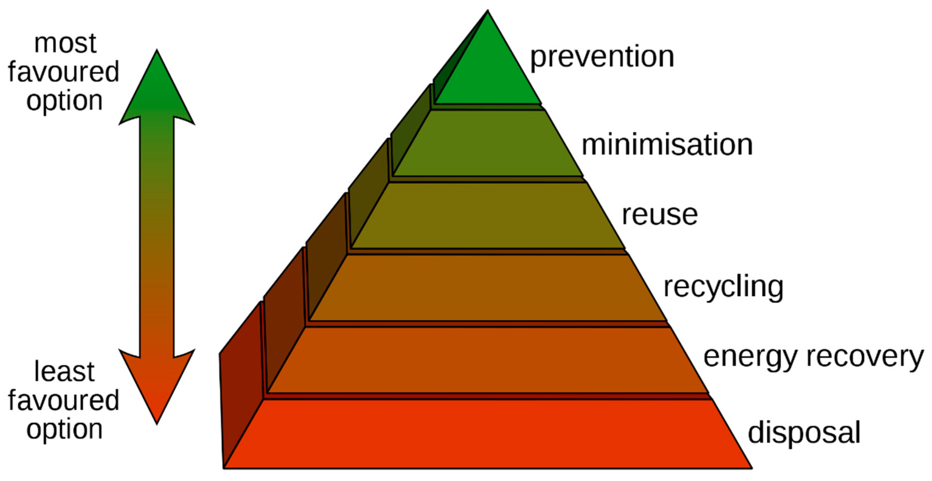
One of the major challenges of the 21st century is the continuous increase of municipal solid waste (MSW) production as well as its management. According to the European Union (EU) Waste Framework Directive (WFD) 2008/98/EC, ‘any substance or object which the holder discards or intends or is required to discard’ is defined as waste. The main treatment options for MSW include, among others, landfill, incineration, recycling and composting. Both developed and developing countries have been dealing with the issue of sustainable waste management and are investigating ways to meet national and international standards in order to reduce their overall environmental impact. The main issues that have been pestering developed countries are potential ways to decrease the amount of waste going to landfill and increase the recycling and recovery of materials. The Waste Hierarchy (Figure 1) has been affecting countries’ management options as it gives priority to preventing waste, but even if and when it is created, it should be prepared for reuse, recycling and energy recovering and only disposed to landfill if no other option is possible [1].
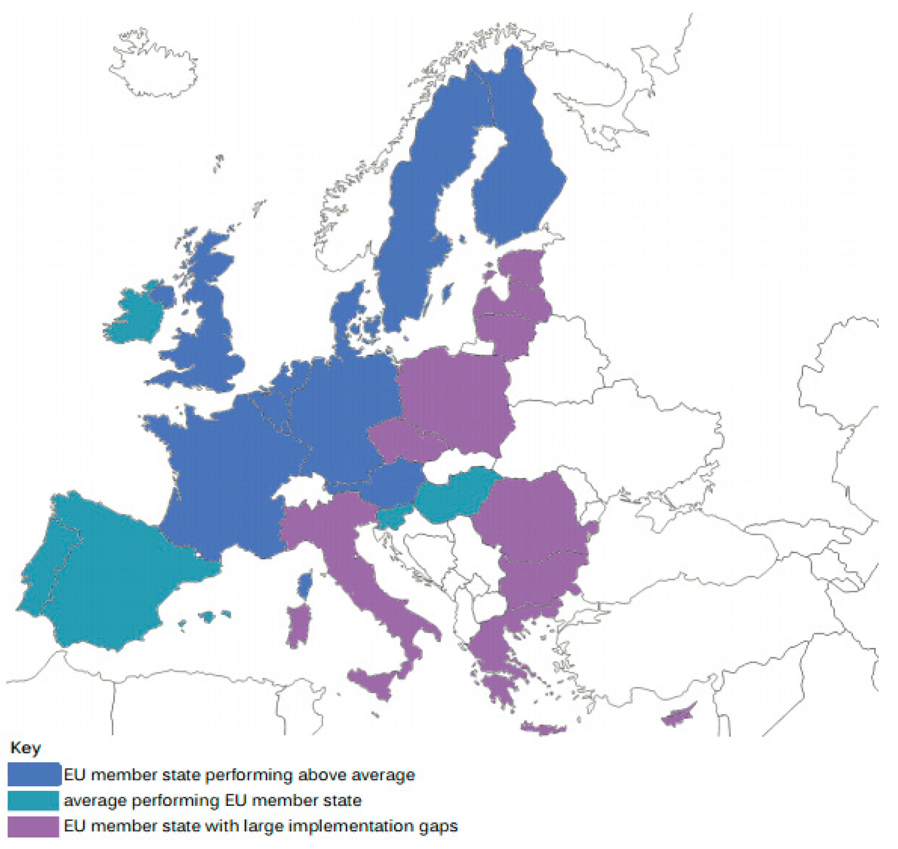
To date many EU Member States have failed to implement waste prevention practices and therefore the regulations that have been set out by WFD [2]. In general Southern and Eastern Europe countries are shown to have the largest implementation gaps regarding their waste management systems [2]. Figure 2 shows EU Member States that have been performing above (blue), below (purple) and average (green) regarding their waste management.
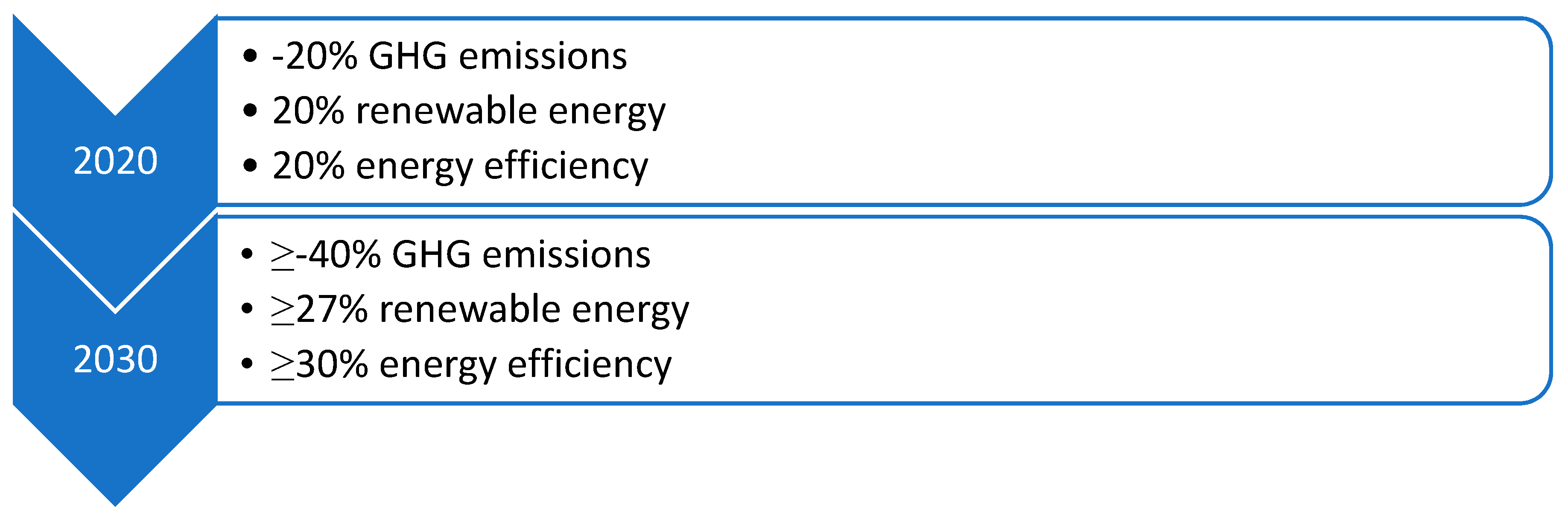
A significant part of the Europe 2020 growth strategy has been sustainable growth towards a ‘smart, sustainable and inclusive economy’ under the notion of the circular economy, while achieving lower greenhouse gas emissions by 20% compared to levels of 1990, generating 20% of its energy from renewable sources and to increase energy efficiency by 20% [3]. These measures could bring net savings to EU Member States, while increasing resource productivity by 30% by 2030, enhancing Gross Domestic Product (GDP) by nearly 1% and creating 2 M additional jobs while also reducing EU carbon emissions by 450 Mt by 2030 [4]. The framework of measures for the promotion of energy efficiency is set out by Directive 2012/27/EU of the European Parliament and of the Council of 25 October 2012 on energy efficiency addressing the achievement of the 20% target on energy efficiency in 2020.
In addition to those, the 2030 climate and energy framework covers EU-wide targets and policy objectives for the period 2021 to 2030, with the main targets being: at least 40% cuts in greenhouse gas (GHG) emissions (from 1990 levels), at least 32% share for renewable energy and at least 32.5% improvement in energy efficiency [5]. Moreover the 2050 EU long-term strategy stresses the opportunities that a climate neutral Europe may bring as well as challenges that may appear, without revising the 2030 targets nor launching new policies [6]. Overall this strategy is meant to provide a framework for the EU to achieve the Paris Agreement objectives and tackle climate change by limiting global warming to below 2 °C and attempting to limit it to 1.5 °C [6].
Generally it is noticed that the global economy is highly reliant on fossil fuels such as oil, gas and coal, resulting in higher GHG emissions [7,8]. Due to the volatile price of oil and the environmental degradation occurring because of fossil fuels’ use, a turn towards renewable energy sources has been noticed [9]. Along those lines the public has become more sensitive to environmental issues, therefore most countries will be forced to make real changes in their energy mix [10].
Energy efficiency improvement can provide many benefits apart from cost efficiency such as energy savings, air pollution control and GHG emission reduction as well as energy security and health benefits [11,12]. It is essential to combine technological options and implementation approaches to improve energy recovery efficiency of the urban and industrial system and achieve low-carbon cities [13]. In those regards, the development of advanced computational techniques has enabled the evaluation of energy efficiency [14].
Such a tool is data envelopment analysis (DEA) which has been accepted throughout the academic community as a useful benchmarking technique [14]. DEA is a non-parametric linear programming method used to measure the efficiency of selected decision making units (DMUs) [15]. Initially it was intended to be applied in microeconomic studies, but comes handy in macroeconomic analysis too [16].
In the present paper DEA was used at a macroeconomic level, to evaluate energy efficiency in 28 selected EU Member States with the aim to identify the current levels of efficiency as well as to assess the potential of using MSW to regain energy and ensure reliable supplies for all at reasonable prices with the least potential impacts taking the financial crisis into account too. The existing literature shows that there is a major gap in current research as researchers have not attempted to evaluate energy efficiency among EU Member States in order to understand what this means and its potential implications for the MSW sector especially under the circular economy concept. This study therefore aims to also provide EU energy efficiency levels that could act as an incentive to move more towards energy recovery from waste and realise a circular economy in full.
Apart from this Introduction, the rest of the paper is structured as presented below. Section 2 provides the background research on this topic by reviewing the main elements of energy recovery from waste (Section 2.1) as well as the relevant existing DEA studies (Section 2.2) with Section 3 showing the proposed methodology along with the data used. Section 4 presents the empirical findings while Section 5 analyses the results and their implications. Finally the last section (Section 6) concludes the paper.
2. Background
This section provides some main points to introduce the topic of energy recovery from waste and the various options with which this can be made (Section 2.1). Then Section 2.2 reviews some of the studies that have used DEA in evaluating energy efficiency, leading to the methodology part in the following section, Section 3.
2.1. Energy Recovery from Waste
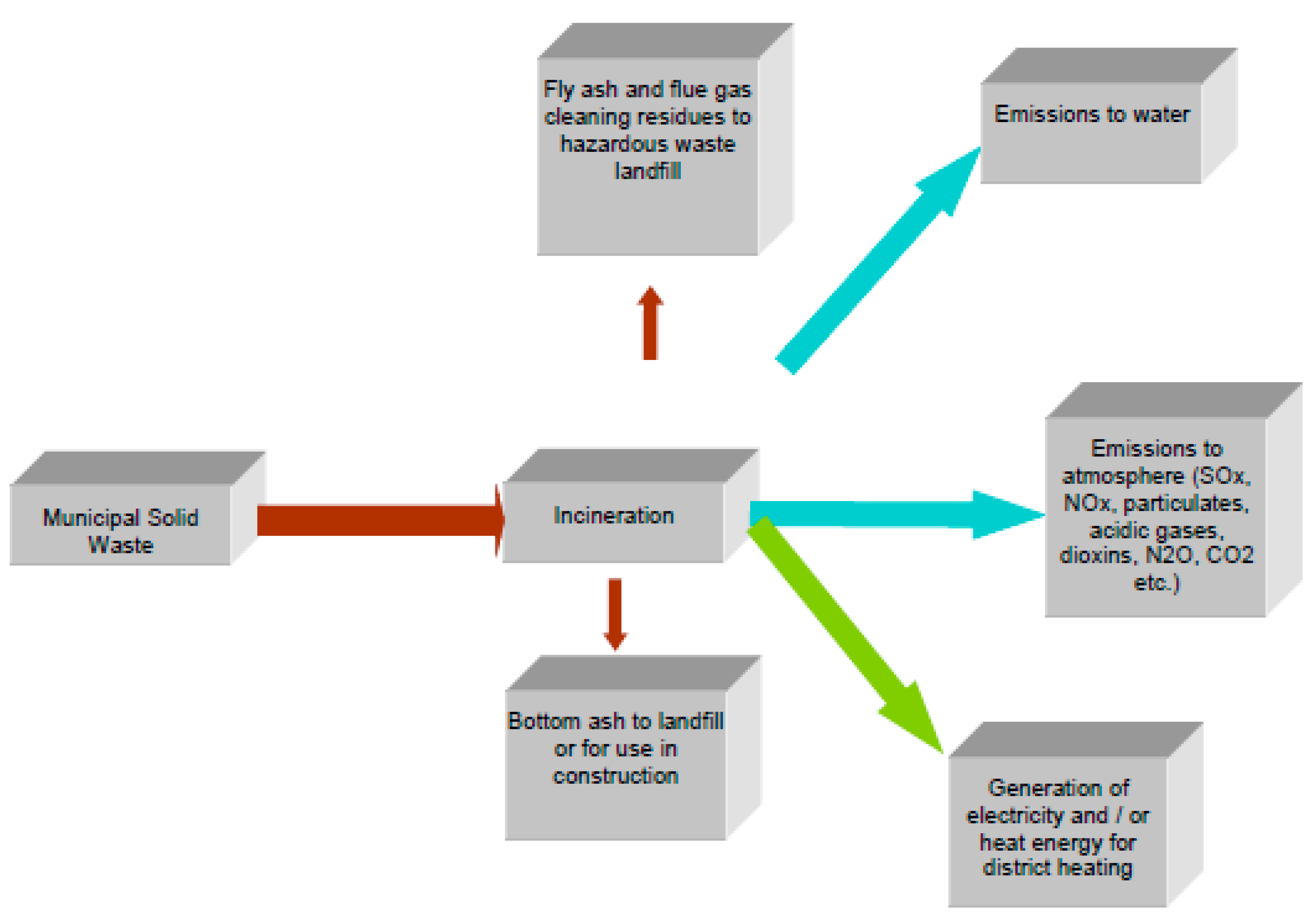
As already mentioned, the burning of waste for recovering energy is called incineration and it happens under a high temperature, therefore it is also called thermal treatment [17]. MSW can act as a source of energy through waste incineration; for instance in Denmark waste incineration covers approximately 5% of the electricity demand and 20% of the district heating demand [8]. With the use of incineration wastes’ form is reduced from 95 to 96%, depending how many materials can be recovered as well as their composition; therefore incineration does not achieve the omission of landfill completely but reduces the amount of waste disposed that way [17]. Figure 3 presents the main inputs and outputs from incineration.
In 2009 there were 449 Incineration plants across 20 Western and Central European countries with a total throughput of around 69.4 Mt [19]. In 2016 there were 512 plants in Europe alone, providing a total incineration capacity of 93 Mt [20]. In many countries such as Germany and Japan, incinerators are widely used to treat both MSW and industrial waste [21]. Incineration has been raising a lot of controversy regarding its potential use. Generally public disagreement can affect political willingness to support incineration, which has been the case especially for Spain and Greece [22].
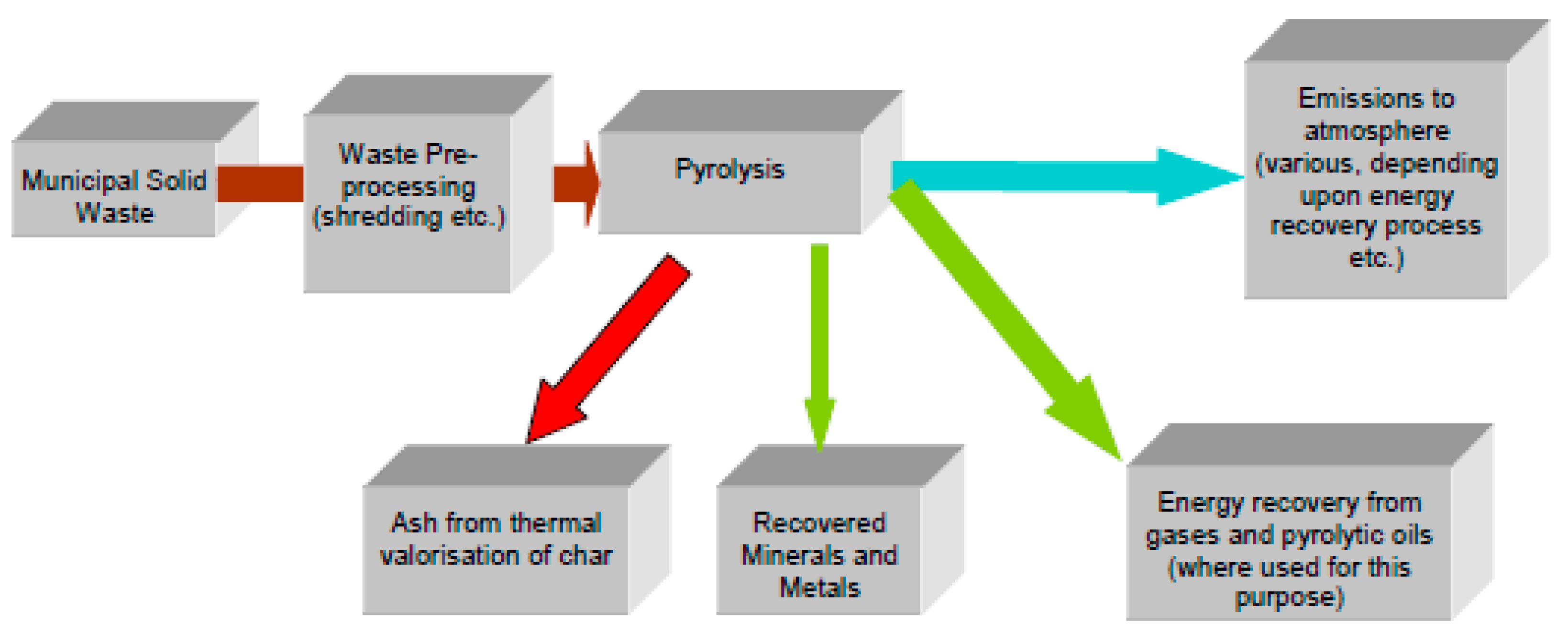
Some other relatively new technologies include pyrolysis and gasification but these have not yet been fully employed in the EU [18]. Pyrolysis is the thermal decomposition of materials in the absence of oxygen [23]. The pyrolysis of biomass results in the production of char, liquid and gaseous products (Figure 4) [24]. It can be divided into three main parts: conventional pyrolysis, fast pyrolysis and flash pyrolysis [25]. More recently research has focused on fast pyrolysis in which case waste is decomposed quickly under high temperatures and produces bio-oil. The main features of a fast pyrolysis process are [26]:
- very high heating and heat transfer rates
- carefully controlled temperature of around 500 °C
- rapid cooling of the pyrolysis vapours.
Bio-oil that is produced through pyrolysis can replace fuel oil or diesel, for instance in boilers, furnaces, engines and turbines for producing electricity [23]. Even though the production of crude bio-oils has been researched extensively, little progress has been made to produce additives or transportation fuel extenders from these oils, therefore this is an area that has to be further examined [27].
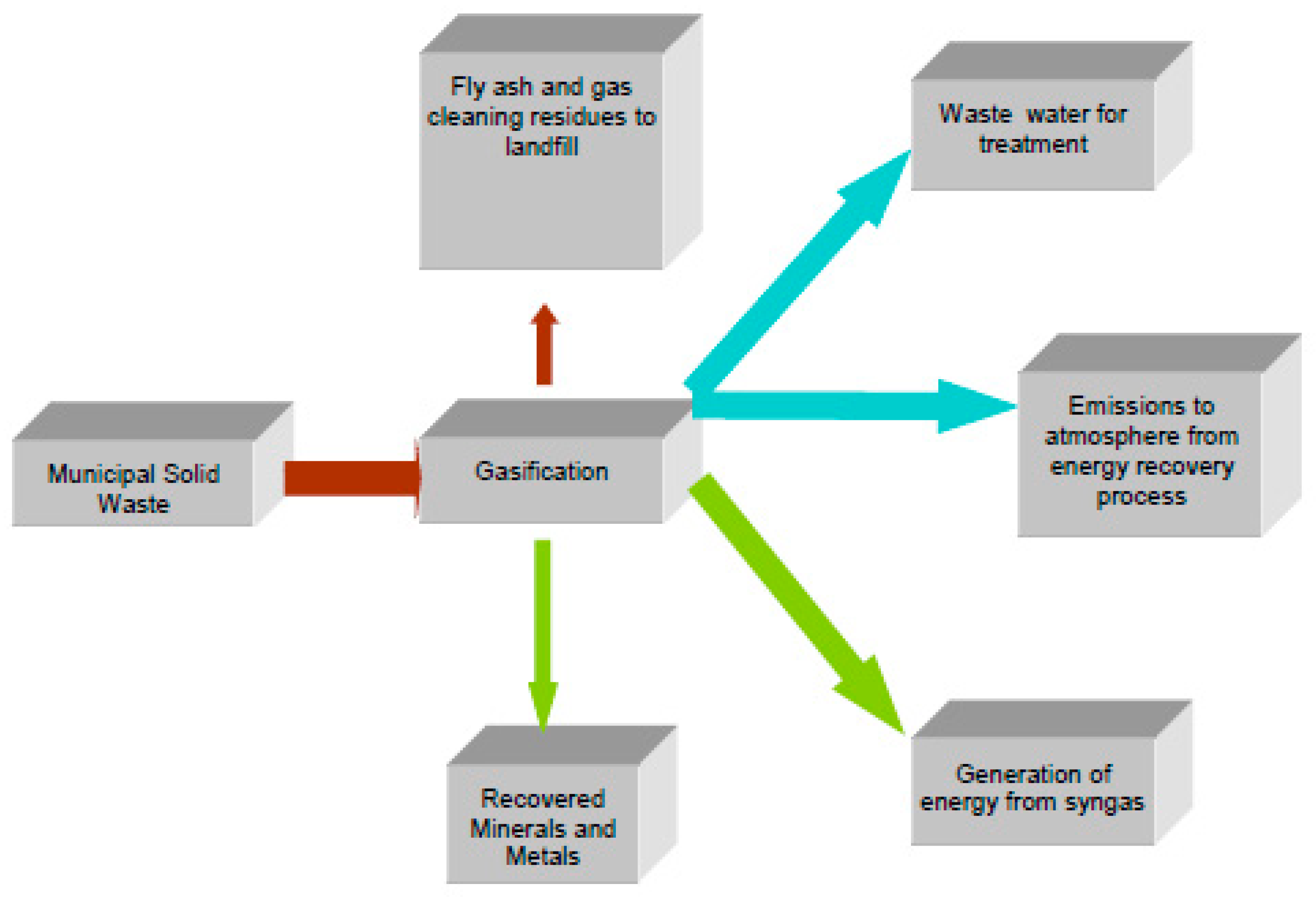
Gasification is actually a process between pyrolysis and incineration because it comprises of the partial oxidation of waste [19]. Gasification involves heating carbon rich waste in sub-stochiometric conditions, whereas the majority of carbon is transformed into a gaseous material leaving an inert residue from the breakdown of organic molecules [18]. In gasification (Figure 5) carbon based wastes are heated in the absence of oxygen to produce a solid, low in carbon and energy from syngas which is a fuel gas mixture consisting of hydrogen and carbon monoxide [19], and can therefore be considered as a thermochemical process. Gasification is highly efficient and has low environmental emission rates therefore it is a quite desirable technology [28]. It is a viable alternative to incineration specifically for thermal treatment of homogeneous carbon-based waste and for pre-treated heterogeneous waste [29].
In addition to the methods described above, a further treatment method is anaerobic digestion (AD) which includes the bacterial decomposition of organic material in almost anaerobic conditions whose by-products include biogas and digestate [18]. There are two main types of anaerobic digestion called thermophilic and mesophilic – the primary difference between them is the temperatures used in the process; thermophilic processes reach temperatures of up to 60 °C whereas the mesophilic ones normally run at about 35–40 °C [30].
The high degree of flexibility associated with AD is considered one of the most important advantages of the method, since it can treat several types of waste, ranging from wet to dry and from clean organics to grey waste [18]. Therefore it’s a quite desirable option, and for instance in the UK alone there were about 378 AD combined heat and electricity (CHP) plants in 2015 [31]. AD (Figure 6) can in comparison to composting better treat waste with a higher moisture content and can occur usually between 60% and 99% moisture content [18]. Hence kitchen waste and other putrescible wastes which are high in moisture can be an excellent feedstock for AD, whereas woody wastes including a higher proportion of lignocellulosic materials are better suited to composting [32].
The process of AD provides a source of renewable energy, since waste is broken down to produce biogas (a mixture of methane and carbon dioxide), which can be used to produce energy. The biogas can be used threefold: to generate electricity, to power on-site equipment and any excess electricity can be exported to the national grid [18]. Possible uses include its potential to provide heat, electricity or both. Alternatively, the biogas can be ’upgraded’ to pure methane, often called biomethane, by removing other gases. One cubic metre of biogas at 60% methane content converts to 6.7 kWh energy [33].
Therefore incentives are provided by the EU to encourage small to medium enterprises and farms to employ AD to gain economic benefits from their organic waste; for instance the UK Renewable Heat Incentive (RHI) scheme provides quarterly payments over twenty years for non-domestic thermal energy production using renewable resources [31].
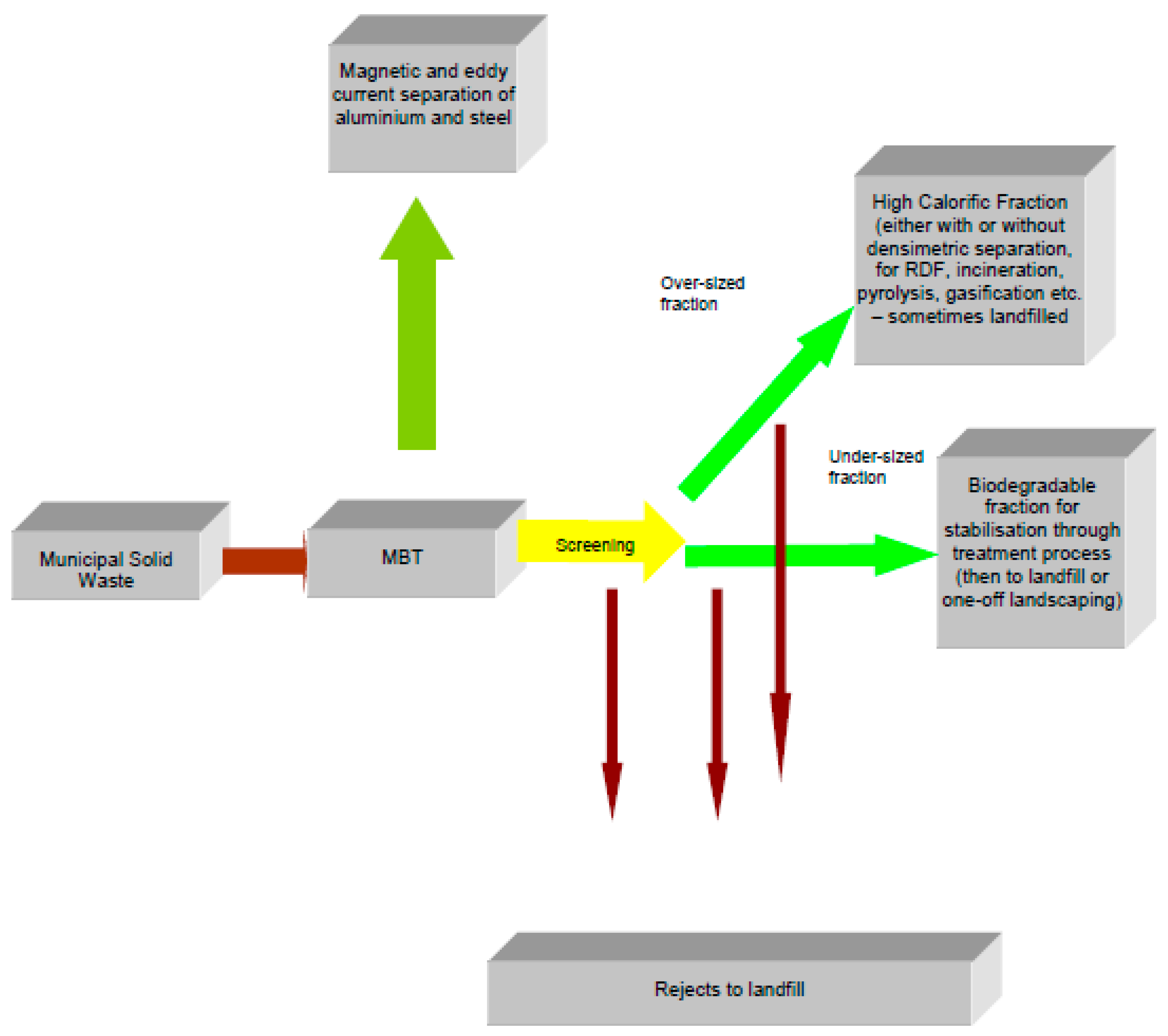
Finally another important waste-to-energy technology is mechanical biological treatment (MBT) through which the so-called refuse derived fuel (RDF) or solid recovered fuel (SRF) can be produced. RDF generally includes sewage sludge, waste wood, calorific fractions of household and commercial waste, shredder lightweight fractions, scrap tyres, food byproducts [34]. MBT is a process designed to optimise the use of resources by recovering materials for one or more purposes and stabilising the organic fraction of residual waste [18].
Some of the benefits of MBT include the fact that materials and energy can be recovered, space requirements are reduced and gas and leachate emissions from landfill are reduced at the same time [18]. MBT systems basically comprise of two simple ideas: either to separate the waste and then treat or to treat the waste and then separate [19]. Aerobic biological unit processes are used to ‘stabilise’ the organic fraction, to reduce its biodegradability and therefore its ability to generate methane, whereas anaerobic biological unit processes can help produce biogas from the organic portion of MSW [35]. Figure 7 presents a schematic representation of the MBT inputs and outputs. In those regards RDF must fulfill general quality requirements in order to be safely and efficiently used such as [34]:
- well defined calorific value
- low chlorine content
- quality controlled composition (few impurities)
- defined grain size
- defined bulk density
- availability of sufficient quantities with required specifications.
In relation to the aforementioned information, it should be noted that there is an increasing interest in the development and application of heat recovery systems worldwide, driven by government regulatory requirements both from an environmental and an economic perspective [36]. For instance in the EU, 70% of the total energy use in the industrial sector is for thermal processes and about 1/3 of this energy is waste, which could be recovered and used instead [37].
The waste heat recovery market is projected to continue to rise and thus far the EU is the dominant player accounting for 38% of the global market [36]. Of course every industry shows different potential for waste heat which can be seen in Table 1.
Moreover efficient energy recovery means that access to heat distribution infrastructure which utilises recovered excess heat is essential [38]. Closing this section it should be noted that the EU Commission suggests that more investments should be made to AD processes than incineration, in order to ensure that increases in recycling and reuse do not find any obstacles [39].
2.2. Use of DEA in Energy Efficiency Studies
Many studies have focused on the field of energy and environmental efficiency with the use of DEA. Efficiency is the ratio of output to input; a state of absolute efficiency is achieved when the best possible output per input is realised and it is not possible to amend this without changing technology or any other factors in the production process [35]. Some researchers have composed a list of the main studies working on this topic [40,41]. In more detail, Mardani et al. [40] identified a total of 144 papers between 2006 and 2015. The specific focus of those studies can be seen in Table 2.
Sueyoshi et al. [41] present DEA applications from 1980 to 2010 (693 studies) and a considerable increase in research has been noticed after 2000. The first research work on energy efficiency was by Färe et al. [42]. Further studies focused both on developed countries such as Canada [43], USA [44], selected Organisation for Economic Co-operation and Development (OECD) ones [45,46] and developing countries like Korea [47] and India [48].
These studies have focused on different aspects of energy efficiency. For instance Zhou et al. [45] by using DEA measured the carbon emissions’ performance of eight regions worldwide in 2002, while they examined the environmental efficiency of 26 OECD countries from 1995 to 1997 [45]. Halkos and Tzeremes [7] examined energy consumption on countries’ economic efficiency levels and DEA in that case presents economic efficiency variations among the examined countries. Additionally the effects of renewable energy on the technical efficiency of 45 economies during 2001–2002 was studied by Chen and Hu [49] showing that increasing the use of renewable energy improves an economy’s technical efficiency.
Chen et al. [21] evaluated the performance-based efficiencies of 19 largescale municipal incinerators in Taiwan with different operational conditions for 2002–2005, leading to optimal management strategies for promoting the quality of solid waste incineration. Moreover the renewable energy sector in Greece is examined through DEA for 78 firms for 2006–2008 showing that the majority of the firms operating in the Greek renewable sector are based on the production of wind energy [10].
Hu and Wang [50] measured the energy efficiency of 29 regions in China and propose a total factor energy efficiency evaluation method. The technical efficiency of energy utilities in China and Taiwan was also studied by Yeh et al. [51]. The same approach but with the incorporation of environmental efficiency as well was followed by Bian and Yang [52]. Furthermore Zhou and Ang [53] measured energy efficiency using both energy and non-energy inputs. Wang et al. [54] created a mixed efficiency model which includes both economic and environmental efficiency attempting to proportionally increase desirable outputs and decrease undesirable outputs.
Wang et al. [55] evaluated energy and environmental efficiency of 29 regions in China with an improved DEA model. Yang et al. [56] modeled carbon emissions from travel in Beijing using microsimulation modelling and investigating the effects of the major transport policies. Finally Song et al. [57] developed an improved method by which to evaluate resource and environmental efficiency with the evaluation of resource inputs into the objective function and focus on resource inputs, undesirable outputs and desirable outputs simultaneously.
3. Research Methods, Data and Production Frameworks
3.1. The Proposed Methodology—An Overview of DEA
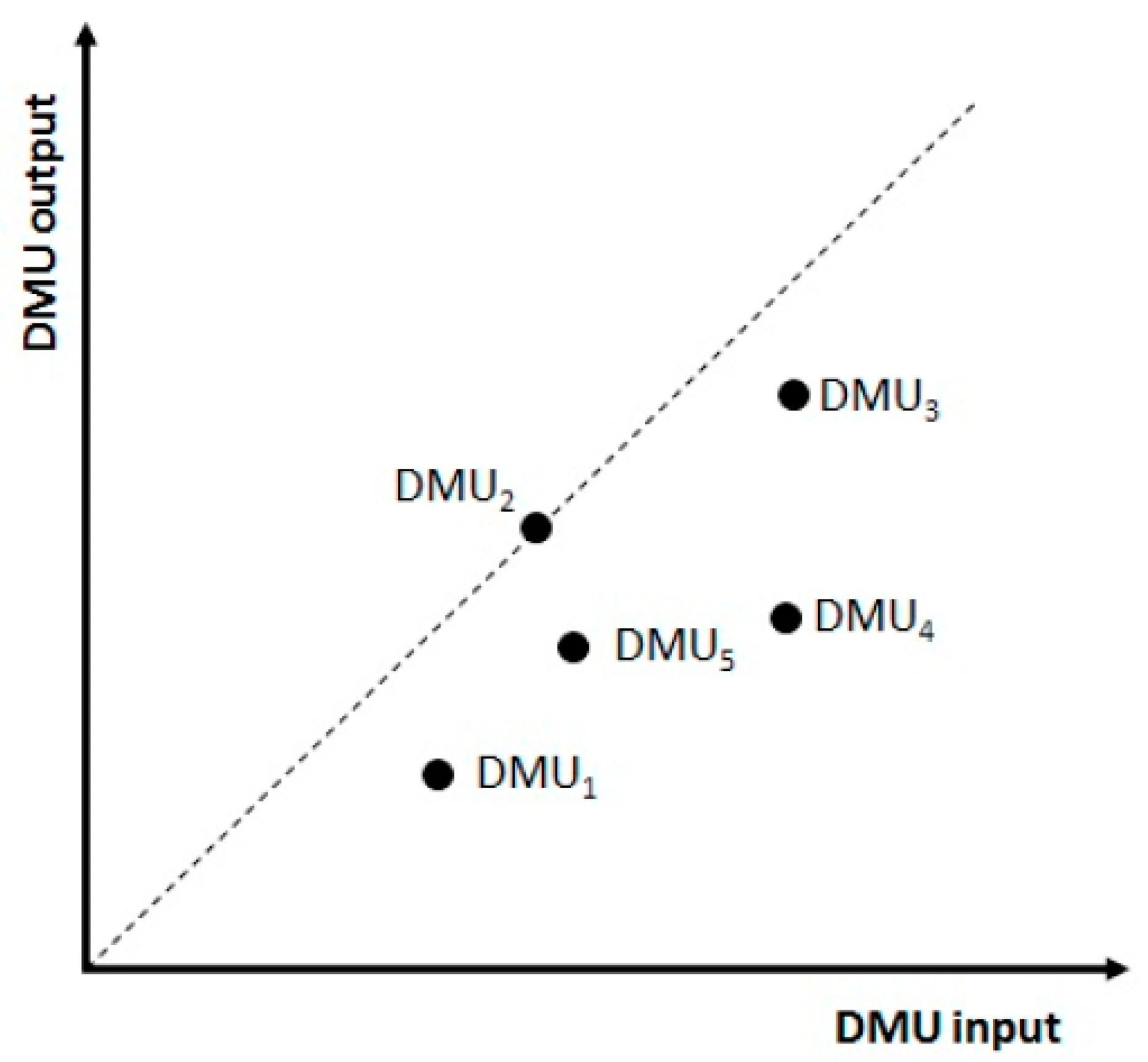
As mentioned already DEA is used to assess the efficiency of selected DMUs, whereas each unit is compared with all others [12] and aims to identify the ones that are operating inefficiently [35]. That way both good and bad outputs can be taken into account [15]. Efficient DMUs achieve a rating of 1 (or 100%) and these constitute the efficiency frontier showing the non-efficient DMUs as well [12,58].
In DEA analysis it is not necessary to assume that there is any specific relationship between inputs and outputs [59]. DEA models are either input-oriented minimizing inputs or output-oriented models maximizing outputs without the use of more inputs [60]. The relevant formulations of those two models are as follows [14]:
Input-oriented Min
Subject to:
Output oriented Max
Subject to:
where θ0 is DMU 0’s efficiency score, is DMU k’s contribution on the targets of DMU 0, yj0 is output j quantity for DMU 0, xi0 is output i quantity for DMU 0 and n is the quantity of DMUs used on the model. Moreover the decision varialbes are θ and λ. Farrell’s [61] input measure operationalization of efficiency was introduced via linear programming estimators by Charnes et al. [62]. Therefore for a given DMU operating at a point it can be defined as:
where x and y are the input and output vectors.
DEA has been widely used in research mainly because one can use multiple inputs and outputs without assigning weights on those and at the same time efficiencies are calculated based on the best operating DMU and not on average performance levels [63]. On the contrary a disadvantage of DEA is that is that it produces a separate linear programme for each DMU thus creating a computational mess when there are a lot of DMUs taken into account [60].
3.2. Bias Correction and Returns of Scale in DEA
Bootstrap is used in most DEA studies as the DEA estimators have been proven to be biased by construction so it is necessary to correct and estimate the relevant bias [64,65,66]. In that case a simulation of the data generating process (DGP) is applied whereas the estimator copies the sampling distribution of the original estimator [67]. At the same time the sensitivity of the efficiency scores relative to the sampling variations of the estimated frontier is defined as well [64].
The bootstrap bias estimate for the original DEA estimator θ DEA (x, y) can be calculated as:
where B stands for bootstrap replications performed.
The biased corrected estimator of (x, y) can be calculated as:
This procedure also provides confidence limits on the efficiencies in order to present the true efficient frontier within the specified interval [68]. Therefore the (1−α) × 100—percent bootstrap confidence intervals can be obtained for θ(x, y) as:
These calculations have also been applied in this research as will be presented in Section 4.
Another important element that needs to be considered in the DEA analysis is if constant returns to scale (CRS) or variable returns to scale (VRS) deem suitable for each specific case. Under CRS as originally designed by Charnes et al. [62] (CCR model) a full proportionality between all inputs and outputs is assumed [69] which could be the case when firms operate at the optimal level [70]. It is possible to disregard this information by using VRS. As originally designed by Banker et al. [71] (BCC model) VRS accounts for the use of technical and scale efficiencies in DEA. This method includes both increasing and decreasing returns to scale. Therefore following Simar’s and Wilson’s [64] bootstrap approach we compare between CRS and VRS according to these hypotheses:
Ho : Ψθ is CRS
H1 : Ψθ is VRS
The test statistic mean of the ratios of the efficiency scores is then provided by:
Then the p-value of the null-hypothesis can be obtained:
where Tobs is the value of T computed on the original observed sample Xn and B is the number of bootstrap reputations. Then the p-value can be approximated by the proportion of bootstrap values of T*b less the original observed value of Tobs such as:
Based on these equations, calculations have been performed on Stata and it is shown that for the data used (Section 3.3) and the designed frameworks (described in further detail in Section 3.4), CRS is more appropriate following the CCR model [62] as the results obtained are higher than 0.05 thus accepting the null hypothesis (B = 999). The specific results are shown in Table 3.
In the case of the CRS or CCR models, the efficiency frontier is a straight line crossing the point of origin and the best performers (efficient DMUs) [72]. Figure 8 presents the graphical representation of the efficient and inefficient DMUs along the frontier, in which case DMU2 is the best performer and is used as a reference for all other DMUs. In those regards further improvement of efficiency scores for inefficient DMUs can be achieved through the implementation of good practices of the efficient ones [73].
3.3. Data Used
For this paper’s analysis the MaxDEA for Data Envelopment Analysis programme (MaxDEA Basic 6.6 – 2015 edition) is used. Table 4 presents the descriptive statistics of the inputs and outputs used in the different DEA frameworks and for all the years and for all the examined countries.
In this analysis the variables used include: final energy consumption, GDP, labour, capital, population density, nitrogen oxide (NOx) emissions (from energy), sulphur oxide (SOx) emissions (from energy) and GHG emissions (from energy) with data obtained from Eurostat. In total 28 EU Member States are examined for the years 2008, 2010, 2012, 2014 and 2016. The following units are used for each factor of this analysis:
- Final energy consumption: Mt equivalent
- GDP: current prices (M Euro)
- Labor: number of persons (thousand persons)
- Capital: gross fixed capital formation (current prices, M Euro)
- Population density: persons per km2
- SOx emissions: t (from energy production and distribution)
- NOx emissions: t (from energy production and distribution)
- GHG emissions: thousand t of CO2 equivalent (from energy production and distribution)
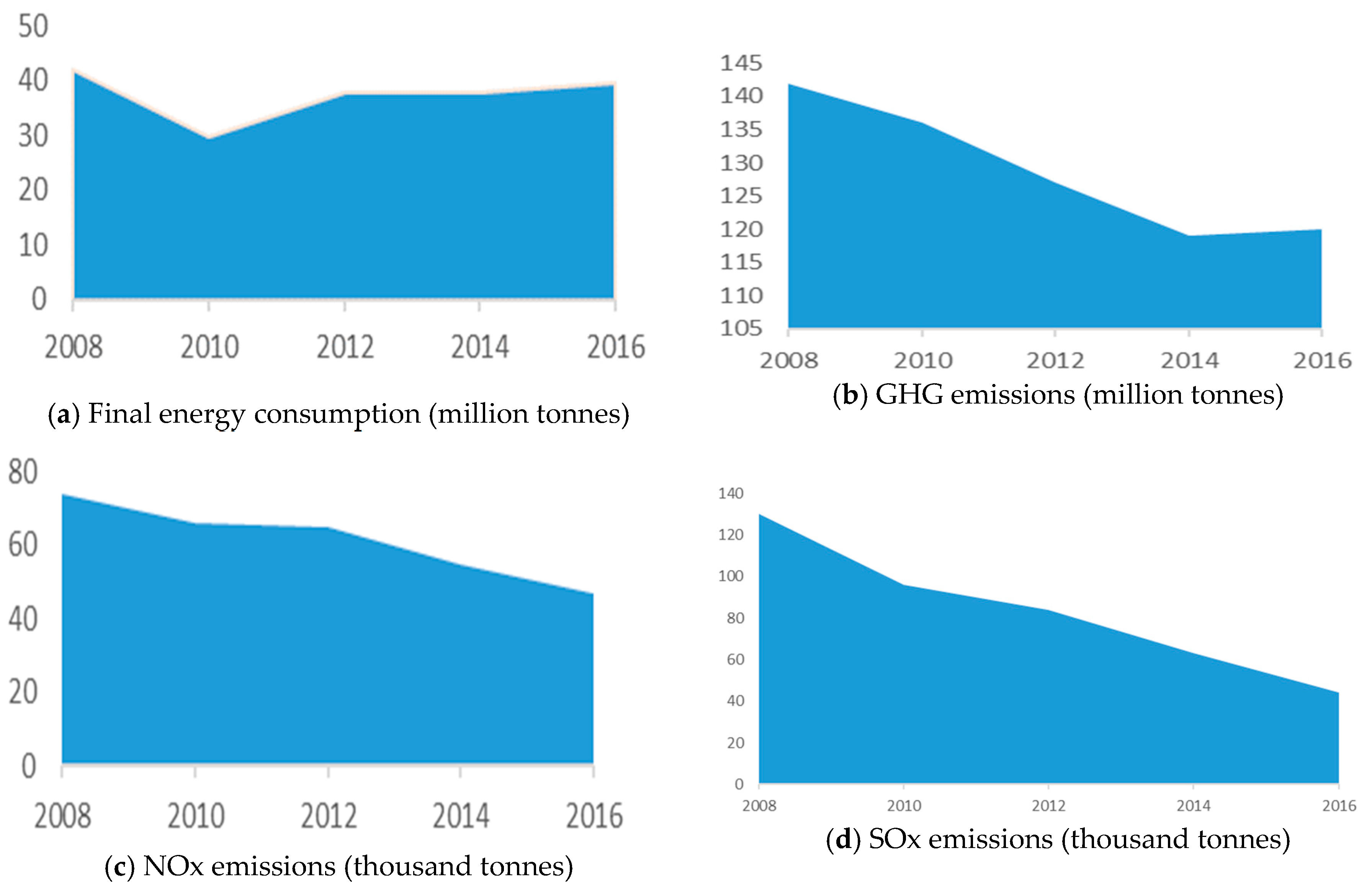
Based on these data, Figure 9 presents the trend of energy consumption levels, SOx, NOx and GHG emissions for all examined years on an average EU basis for the 28 countries taken into account. It is noticed that all indicators have dropped since 2008 especially SOx and NOx emissions, while energy consumption and GHG emissions are on the rise again after 2014.
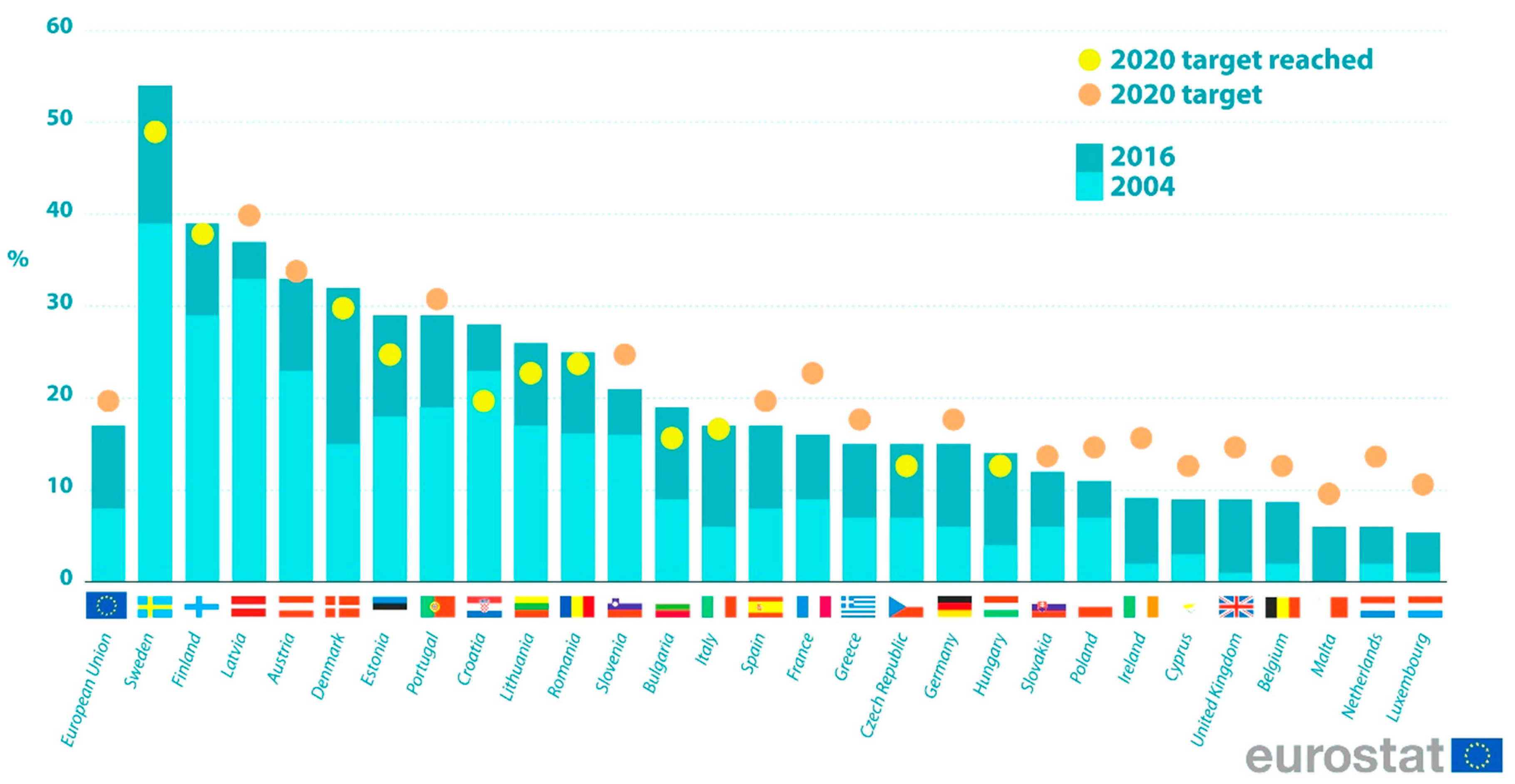
At the same time it is noticed that the share of energy from renewable sources is also on the rise in the EU Member States as shown in Figure 10, showing also how far those countries are from achieving their 2020 target. So far Sweden, Finland, Denmark, Estonia, Croatia, Lithuania, Romania, Bulgaria, Italy, Czech Republic and Hungary have managed to accomplish this.
3.4. Environmental Production Frameworks
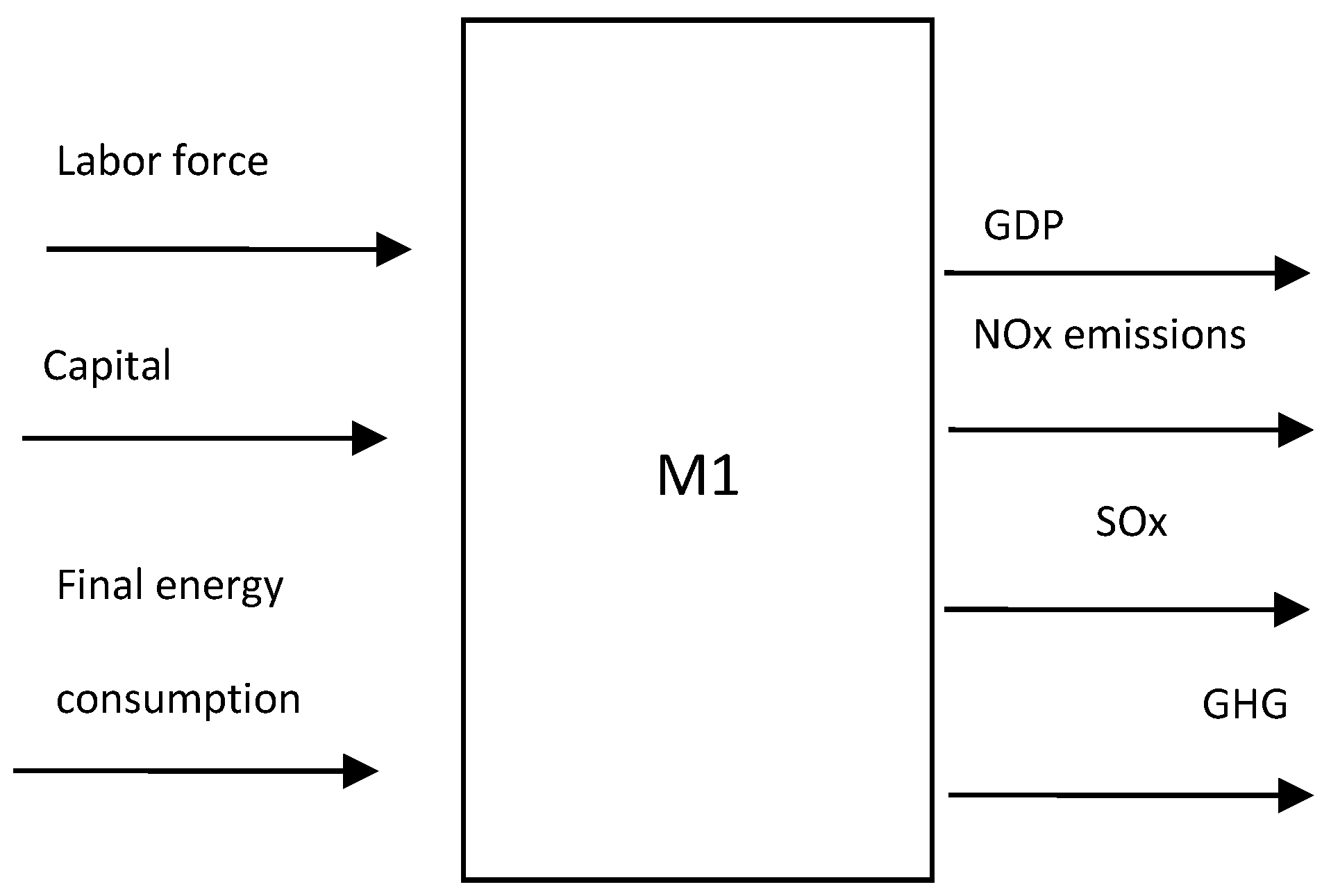
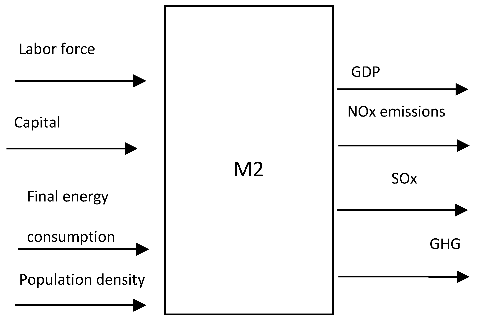
Following studies such as those of Wang et al. [55] and Chien and Hu [74], where capital, labor, population density (M2 framework) and energy consumption are used as inputs and GDP (desirable output), carbon dioxide and sulphur dioxide (undesirable outputs), this paper’s analysis produces two production frameworks as presented in Figure 11 (M1 framework) and Figure 12 (M2 framework). Population density is a factor that has not been used in previous research regarding energy efficiency but it is a strong inequality measure which affects regional and interregional policies and in turn regional and interregional socioeconomic development [50]. In both frameworks a radial model is used, which is output oriented (as presented in Section 3.1).
Overall to evaluate the energy efficiency of the studied EU Member States, DEA was used to examine all countries’ parameters, classify and quantify the variables, model the problem and determine the best performing DMUs. These were then analysed and recommendations are provided.
4. Result
Under the M1 framework the highest performers are: Hungary, Luxembourg, Sweden; whereas the lowest performers are: Estonia, Bulgaria, Greece and Slovenia. For framework M2 the picture is quite similar. Table 5 shows the efficiency scores of all examined countries for the whole time period studied. Also Table 6 presents the average scores (year-wise) per country per modelling framework.
The obtained results are biased and therefore following the bootstrap technique presented in Section 3, the bias corrected results need to be applied in our analysis. Table A1 and Table A2 (Appendix A) present the efficiency scores of the 28 countries, the bias corrected efficiency scores and the 95-percent confidence intervals: lower and upper bound obtained by B = 999 bootstrap replications using the algorithm described in Section 3.2.
According to the bias corrected efficiency measures the countries with the higher environmental efficiency scores (i.e., >0.497) over the years are reported to be:
- Framework M1: Bulgaria, Cyprus, Estonia, Greece, Lithuania, Malta and Slovenia.
- Framework M2: Bulgaria, Cyprus, Estonia, Greece, Lithuania and Slovenia.
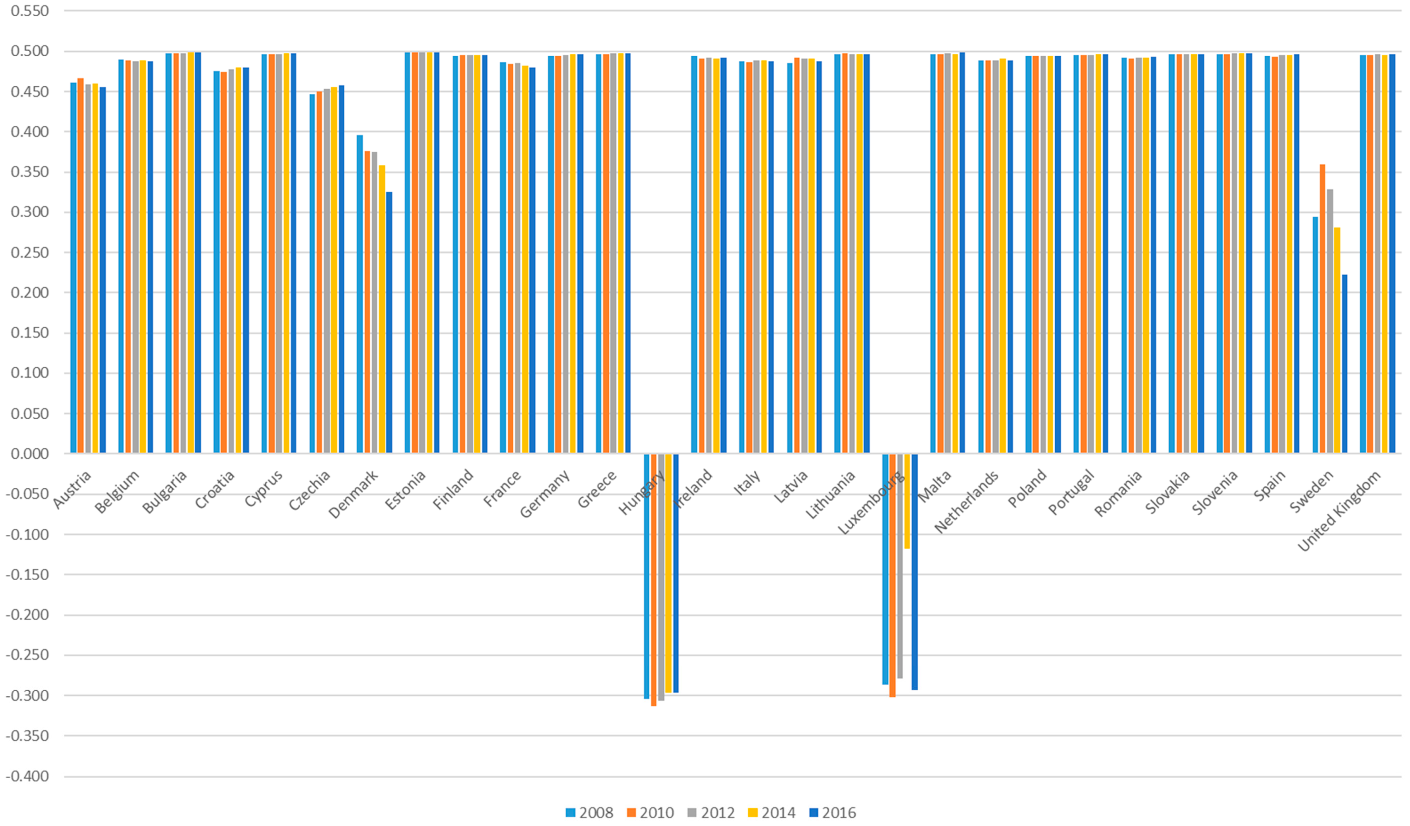
The two modelling techniques used in this analysis cannot be compared to each other since they use different inputs and outputs. A lack of common environmental policies among EU Member States can be seen in their energy efficiency levels regarding energy consumption and the relevant emissions. With regards to changes over the years and as can be seen in Figure 13, most countries seem to maintain their efficiency scores with only Czech Republic, Finland, Ireland, Malta, Romania and Slovenia marginally improving theirs. At the same time, it can be noticed that most countries have higher environmental efficiency scores over 2010 and 2012 with a decrease after that.
5. Discussion
The efficiency scores obtained and presented in the previous section show that EU-wise environmental efficiency levels regarding energy consumption and emissions tend to be quite low. The world’s tension level of energy supply is worsened over the years and efforts are being made to replace traditional fossil fuels with more sustainable options achieving a good balance between economic development and environmental protection [75]. Energy from waste is the largest source of renewable energy today in the EU and is expected to hold this place until 2030, reaching a share of 60–70% [40].
The ‘International Energy Efficiency Scorecard’ published in 2014 by the American Council for an Energy-Efficient Economy stresses that countries can maintain their resources, address global warming, stabilize their economies and reduce the costs of their economic outputs by using energy more efficiently [76]. This can be seen graphically also in Figure 9 where a decrease in emissions’ level is generally noticed. The results obtained from the current analysis are also in connection with the EU’s targets for energy and climate as presented in Figure 14.
In connection to that, nations have been moving towards waste-to-energy with two main objectives, namely sufficient and sustainable energy production and effective treatment of MSW by reducing its volume by about 87% [78]. Both these two factors need to be taken into account when considering this option [79]. A major issue to make sure this option is viable, both from an economic and an environmental perspective, is to take into consideration the resource characteristics, such as their location, amount and quality [80]. The results of this study presenting energy efficiency should be considered to avoid unnecessary entropy production but also to make processes more cost effective and ecofriendly [81]. The main benefits from waste-to-energy include [82]:
- It transforms waste from a problem into a resource.
- Energy generated contributes to primary energy savings from other energy sources.
- It can reduce greenhouse-gas emissions when it replaces more carbon-intensive energy sources.
- Waste to landfill is reduced heavily.
- Waste treatment time is extremely short compared with landfills.
- It also enables treatment of hazardous waste.
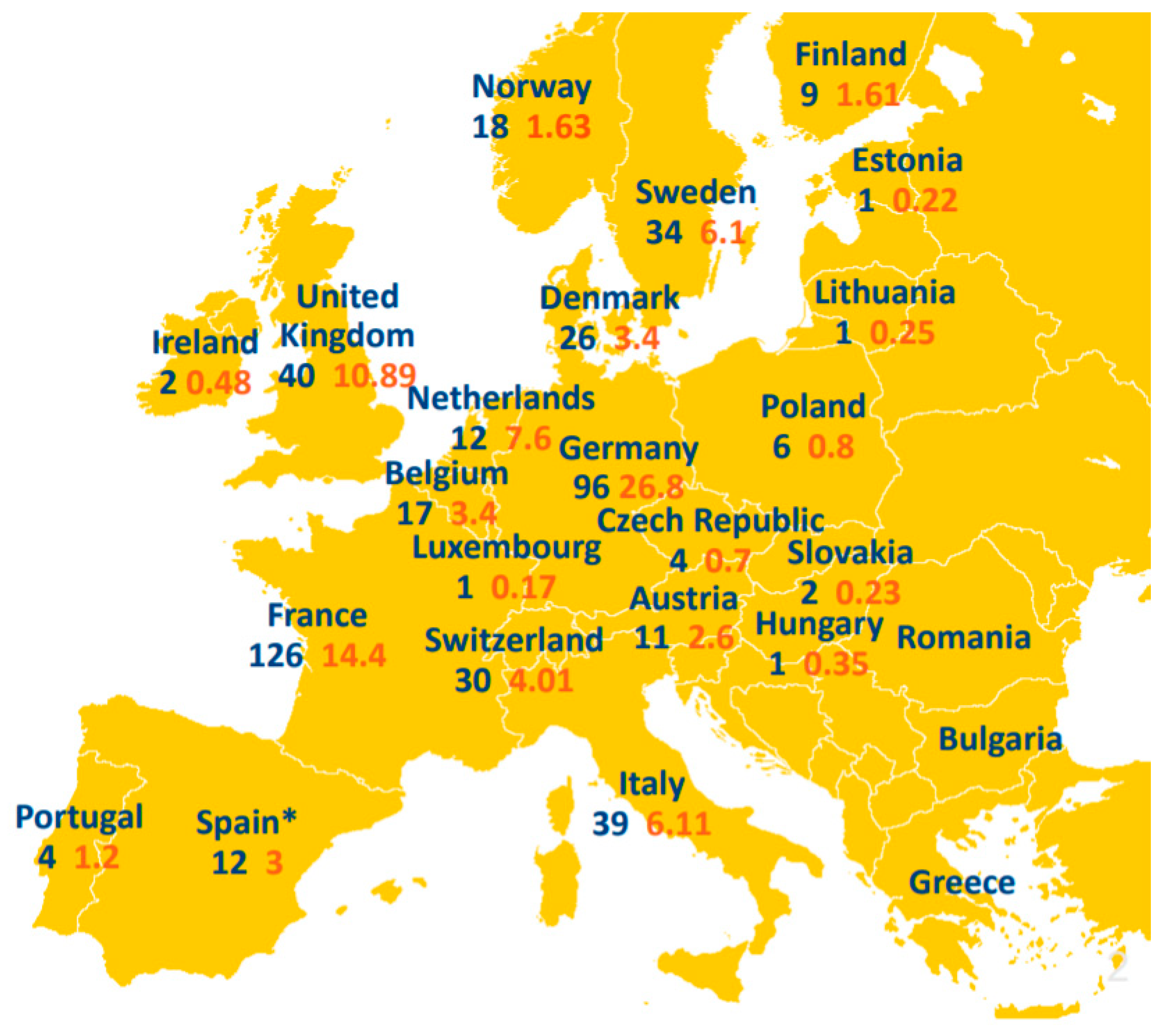
At the same time, the main associated risk is that those systems become highly dependent on and justify societies’ increasingly uneconomical consumption levels, while also having unintended negative effects (such as higher levels of energy and material use throughout a society, increasing upstream environmental impacts) [82]. Moreover it is essential to create a network of the waste by-products, electricity and heat between multiple sectors throughout the world [83,84]. Figure 15 presents a map of waste-to-energy plants in Europe for 2017, in which capacity is seen to be overall stable compared to 2016, with only the UK increasing its capacity.
The necessary treatment that is to be used depends highly on the nature and volume of the waste stream with the main factor taken into account being its energy content (calorific value) and as a rule of thumb waste-to-energy option should be considered when the incoming waste has an average calorific value of at least 7 MJ/kg [86]. Table 7 presents the average net calorific values for most common MSW waste streams.
Overall the European Commission 2017 (Ref. [38]) recommends the main technologies that could be used [88]:
- co-incineration in combustion plants: with gasification of SRF and co-incineration of the resulting syngas in the combustion plant.
- co-incineration in cement kilns.
- incineration in dedicated facilities:
- ◦
- the use of super heaters and heat pumps
- ◦
- the utilisation of the energy contained in flue gas
- ◦
- distributing chilled water through district cooling networks.
- Bio-methane for further distribution and utilisation.
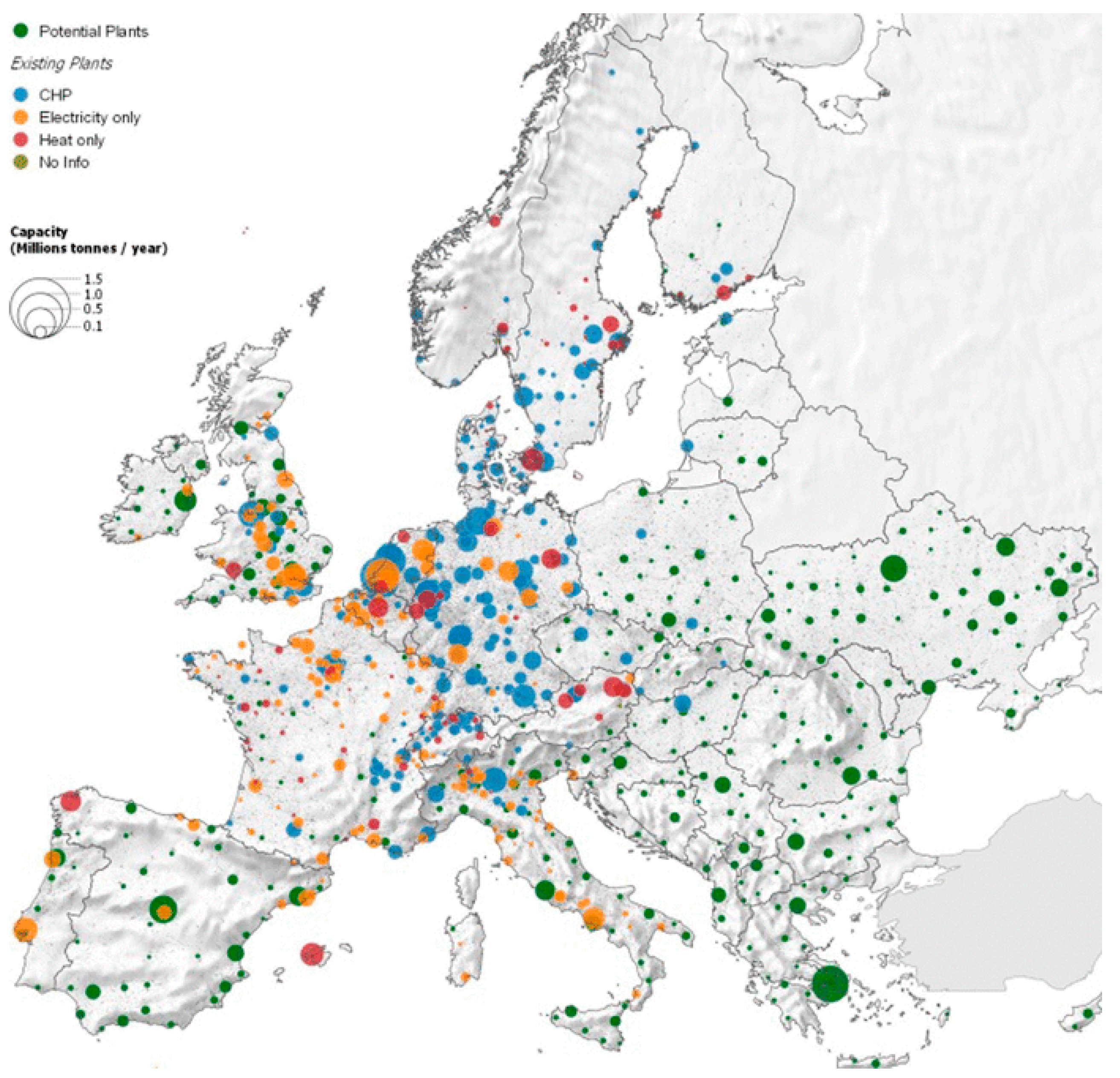
In this regard Scarlat et al. [20] perform a suitability analysis as to where waste-to-energy plants are best to be built, which can be seen graphically on Figure 16. The potential plants (shown in green) are interrelated with the results of the current analysis, as according to their analysis, there is great potential to build plants for instance in the Czech Republic, Croatia, France, Hungary, Italy, Spain and UK. For those countries the current analysis found that energy efficiency scores are overall quite low in comparison to other countries. Also Greece and Bulgaria show a great potential for building waste-to-energy plants which makes sense according to this analysis as for these countries efficiency scores are quite low as well.
Energy efficiency levels across the 28 EU examined countries are quite low overall with only a few differentiated countries. As it stands, waste management is a crucial part in the context of the circular economy whereas prioritization needs to give to prevention, reuse, recycling and energy recovery and as a last resort disposal to landfills [89]. Therefore the circular economy requires a better understanding of existing waste infrastructure, including location and capacity [90]. The circular economy aims to accomplish the optimum production through the 3R principle—reduce, reuse and recycle—while minimizing resource utilization, pollution emissions and waste discarded [91].
To deliver the circular economy governments need to collaborate with various partners to combine scientific research, policies and regulations, thus adopting a long-term policy framework [90]. Along those lines, the EU Commission’s Circular Economy Package drives the treatment options that have been used by EU Member States. This package’s aim is the acceleration of Europe’s transition towards circular economy as well as the waste reduction targets across EU Member States [92]. Therefore it is essential to preserve the worth of products, materials and resources in the economy as much as possible and minimize waste generated [4]. Hence waste-to-energy addresses the problems of energy demand, waste management and GHG emissions at the same time, achieving a circular economy system [93]. By 2020 196 billion kWh of sustainable energy could be produced through waste-to-energy plants which makes an equivalent of the energy produced by 6-9 nuclear stations or 25 coal power plants [94].
At the same time one of the EU Commission’s priorities is also a European Energy Union which ensures reliable energy supplies at rational prices for businesses and consumers and with the least environmental impacts [95]. This union would enhance the economy and attract investments thus creating new jobs opportunities [77]. Competition policy in the EU is essential for the internal market with the first liberalisation directives established in 1996 (electricity) and 1998 (gas) and the second liberalisation directives adopted in 2003 [95]. This competition policy aims mainly to ensure that companies compete fairly, providing more choices to consumers and helping reduce prices and improve quality [96,97].
Despite these regulations, markets seem to be largely national and with relatively few cross-border trade, therefore the EU Commission has paid great attention into controlling potential mergers (such as the proposed merger between EDP and GDP in Portugal), into setting up rules for mergers and in controlling state aid to energy companies across the EU [95]. In more detail, it is essential to have an EU competition policy, mainly to achieve [96]:
- Low prices for all: more people can afford to buy products and businesses are encouraged to produce.
- Better quality: competition encourages businesses to improve the quality of goods and services they sell and to attract more customers and expand their market share.
- More choice: businesses will try to make their products unique.
- Innovation: in their product concepts, design, production techniques, services, etc.
- Better competitors in global markets: competition would enhance European companies’ strength outside the EU and enable them to hold their own against global competitors.
Also waste-to-energy could relieve the EU from foreign imports, for instance in 2012 it imported 4 million TJ of natural gas from Russia, whereas waste-to-energy could substitute 19% of Russian gas imports [94]. Unfair competition will only hinder the clean energy transition as far as Member States continue to provide fossil fuel subsidies, such as direct subsidies to uneconomical coal mines, capacity mechanisms for emission intensive power plants, tax relief for company cars or diesel fuel and similar measures [77]. More detailed research conducted in China by Zhang et al. [97] shows that raw material price subsidies increase profits both for recycling and biofuel companies, but investment subsidies only produce greater profits for recycling companies. One important and unexpected issue that needs to be taken into account and has undoubtedly affected energy efficiency in EU Member States is the financial crisis from which the EU has been suffering severely after 2008. This can also be noticed in the efficiency scores obtained through the present analysis, whereas efficiencies have decreased after 2012 when the crisis became more imminent.
As for the future steps, the EU plans for a climate-neutral Europe by 2050 through investments to realistic technological solutions, the empowering of citizens and aligning action in key areas such as industrial policy, finance, or research [6]. In those regards studies suggest that the potential for using heat from waste could be an equivalent to 200 billion kWh per year by 2050 [90]. Therefore it is essential to already have consultations with young people, citizens affected by the energy transition, inventors, social partners and civil society, mayors and other politicians to show the potential of realizing this energy transition [78].
6. Conclusions and Policy Implications
The current paper examines energy efficiency across 28 selected EU Member States and reviews the potential for energy recovery from waste according to the efficiency scores obtained for the examined Member States. The efficiencies are assessed through DEA under CRS and the following variables are examined: final energy consumption, GDP, labour, capital, population density, NOx emissions (from energy), SOx emissions (from energy) and GHG emissions (from energy) from Eurostat data and for the years 2008, 2010, 2012, 2014 and 2016. The two models that are designed use two outputs one desirable (GDP) and one undesirable (aerial gas emissions – GHG, SOx and NOx) with different inputs in each case.
The bias corrected efficiency scores show that overall Bulgaria, Cyprus, Estonia, Greece, Lithuania and Slovenia are efficient under both frameworks. Also most countries seem to maintain their efficiency scores with only the Czech Republic, Finland, Ireland, Malta, Romania and Slovenia marginally improving theirs. At the same time, it can be noticed that most countries have higher environmental efficiency scores over 2010 and 2012 with a decrease after that.
These efficiency scores show that EU-wise environmental efficiency levels regarding energy consumption and emissions tend to be quite low overall, therefore it is suggestible to move towards waste-to-energy with two main objectives, namely sufficient and sustainable energy production and effective treatment of MSW. This option would enhance the circular economy, whereas prioritization needs to give to prevention, preparation for reuse, recycling and energy recovery through to disposal, such as landfilling. Waste to energy addresses the problems of energy demand, waste management and GHG emissions simultaneously.
Together with the EU Commission’s competition strategy, these options would ensure reliable energy supplies at rational prices for businesses and consumers and with the least environmental impacts. Along with these and taking into account the current analysis’ results, it is essential to account for the financial crisis which affects EU since 2008. Namely the efficiency scores show a decrease after 2012 when the crisis became more imminent (Figure 13). Regarding future steps towards a climate neutral Europe, investments into technology along with the empowering of citizens and industry need to be considered.
The models of the present research could be enriched with additional control variables which could incorporate specific characteristics of EU countries, such as their technological level regarding waste management especially, their institutional background and their education level to name a few. Moreover once data become available it would be useful to expand this research with more recent data to better reflect today’s situation.
Author Contributions
For research articles with several authors, a short paragraph specifying their individual contributions must be provided. The following statements should be used conceptualization, G.H. and K.N.P.; methodology, G.H.; software, G.H.; formal analysis, K.N.P.; investigation, K.N.P.; resources, K.N.P.; data curation, K.N.P.; writing—original draft preparation, K.N.P.; writing—review and editing, G.H. and K.N.P.; supervision, G.H.; project administration, G.H.; funding acquisition, K.N.P.
Funding
This research was funded by the General Secretariat for Research and Technology and the Hellenic Foundation for Research and Innovation (HFRI).
Acknowledgments
This work has been supported by the General Secretariat for Research and Technology and the Hellenic Foundation for Research and Innovation (HFRI). Thanks are due to the three anonymous reviewers and the Editors for their helpful and constructive comments. Any remaining errors are solely the authors’ responsibility.
Conflicts of Interest
The authors declare no conflict of interest.
Appendix A

Table A1.
Bias corrected efficiency scores of countries’ by modelling framework. Framework M1.
| Country | Score Original | Bias Corrected | Bias | Std | Lower | Upper | 2008 |
|---|---|---|---|---|---|---|---|
| Austria | 0.528 | 0.461 | 0.067 | 0.027 | 0.402 | 0.498 | |
| Belgium | 0.507 | 0.490 | 0.017 | 0.006 | 0.475 | 0.499 | |
| Bulgaria | 0.501 | 0.498 | 0.004 | 0.001 | 0.494 | 0.499 | |
| Croatia | 0.515 | 0.475 | 0.040 | 0.012 | 0.439 | 0.493 | |
| Cyprus | 0.502 | 0.496 | 0.006 | 0.002 | 0.491 | 0.499 | |
| CzechRepublic | 0.534 | 0.446 | 0.087 | 0.026 | 0.367 | 0.484 | |
| Denmark | 0.567 | 0.396 | 0.171 | 0.052 | 0.241 | 0.474 | |
| Estonia | 0.501 | 0.499 | 0.002 | 0.001 | 0.496 | 0.500 | |
| Finland | 0.503 | 0.495 | 0.009 | 0.003 | 0.486 | 0.499 | |
| France | 0.510 | 0.486 | 0.023 | 0.008 | 0.465 | 0.498 | |
| Germany | 0.504 | 0.494 | 0.010 | 0.003 | 0.485 | 0.499 | |
| Greece | 0.502 | 0.496 | 0.006 | 0.002 | 0.491 | 0.499 | |
| Hungary | 1.000 | −0.304 | 1.304 | 0.385 | −1.490 | 0.248 | |
| Ireland | 0.504 | 0.494 | 0.010 | 0.003 | 0.484 | 0.498 | |
| Italy | 0.508 | 0.487 | 0.021 | 0.006 | 0.468 | 0.496 | |
| Latvia | 0.511 | 0.485 | 0.025 | 0.010 | 0.463 | 0.499 | |
| Lithuania | 0.502 | 0.496 | 0.006 | 0.002 | 0.491 | 0.499 | |
| Luxembourg | 1.000 | −0.287 | 1.287 | 0.331 | −1.037 | 0.255 | |
| Malta | 0.502 | 0.497 | 0.005 | 0.002 | 0.492 | 0.499 | |
| The Netherlands | 0.508 | 0.489 | 0.019 | 0.007 | 0.472 | 0.498 | |
| Poland | 0.504 | 0.494 | 0.010 | 0.003 | 0.485 | 0.498 | |
| Portugal | 0.503 | 0.495 | 0.008 | 0.002 | 0.488 | 0.499 | |
| Romania | 0.505 | 0.492 | 0.013 | 0.004 | 0.480 | 0.498 | |
| Slovakia | 0.502 | 0.496 | 0.006 | 0.002 | 0.491 | 0.499 | |
| Slovenia | 0.502 | 0.497 | 0.005 | 0.002 | 0.492 | 0.499 | |
| Spain | 0.503 | 0.495 | 0.009 | 0.003 | 0.487 | 0.499 | |
| Sweden | 0.649 | 0.294 | 0.355 | 0.142 | −0.025 | 0.490 | |
| United Kingdom | 0.503 | 0.495 | 0.007 | 0.002 | 0.489 | 0.499 | |
| 2010 | |||||||
| Austria | 0.523 | 0.466 | 0.057 | 0.020 | 0.415 | 0.495 | |
| Belgium | 0.507 | 0.489 | 0.018 | 0.006 | 0.472 | 0.498 | |
| Bulgaria | 0.501 | 0.498 | 0.004 | 0.001 | 0.494 | 0.499 | |
| Croatia | 0.516 | 0.475 | 0.042 | 0.013 | 0.437 | 0.494 | |
| Cyprus | 0.502 | 0.496 | 0.006 | 0.002 | 0.491 | 0.499 | |
| CzechRepublic | 0.532 | 0.449 | 0.082 | 0.024 | 0.375 | 0.484 | |
| Denmark | 0.579 | 0.376 | 0.203 | 0.061 | 0.192 | 0.466 | |
| Estonia | 0.501 | 0.499 | 0.002 | 0.001 | 0.497 | 0.500 | |
| Finland | 0.503 | 0.496 | 0.007 | 0.002 | 0.489 | 0.499 | |
| France | 0.510 | 0.485 | 0.026 | 0.009 | 0.461 | 0.497 | |
| Germany | 0.504 | 0.494 | 0.009 | 0.003 | 0.486 | 0.499 | |
| Greece | 0.502 | 0.497 | 0.006 | 0.002 | 0.492 | 0.499 | |
| Hungary | 1.000 | −0.313 | 1.313 | 0.376 | −1.508 | 0.229 | |
| Ireland | 0.506 | 0.491 | 0.015 | 0.005 | 0.478 | 0.498 | |
| Italy | 0.508 | 0.486 | 0.022 | 0.006 | 0.467 | 0.496 | |
| Latvia | 0.506 | 0.492 | 0.014 | 0.005 | 0.479 | 0.499 | |
| Lithuania | 0.502 | 0.497 | 0.005 | 0.001 | 0.492 | 0.499 | |
| Luxembourg | 1.000 | −0.302 | 1.302 | 0.338 | −1.195 | 0.226 | |
| Malta | 0.502 | 0.496 | 0.006 | 0.002 | 0.491 | 0.499 | |
| The Netherlands | 0.508 | 0.488 | 0.020 | 0.007 | 0.470 | 0.498 | |
| Poland | 0.504 | 0.494 | 0.010 | 0.003 | 0.485 | 0.498 | |
| Portugal | 0.503 | 0.495 | 0.008 | 0.003 | 0.487 | 0.499 | |
| Romania | 0.506 | 0.491 | 0.014 | 0.004 | 0.478 | 0.498 | |
| Slovakia | 0.502 | 0.497 | 0.006 | 0.002 | 0.491 | 0.499 | |
| Slovenia | 0.502 | 0.497 | 0.005 | 0.002 | 0.492 | 0.499 | |
| Spain | 0.504 | 0.493 | 0.011 | 0.003 | 0.483 | 0.499 | |
| Sweden | 0.596 | 0.359 | 0.237 | 0.084 | 0.144 | 0.479 | |
| United Kingdom | 0.503 | 0.496 | 0.007 | 0.002 | 0.489 | 0.499 | |
| 2012 | |||||||
| Austria | 0.529 | 0.459 | 0.070 | 0.027 | 0.397 | 0.497 | |
| Belgium | 0.508 | 0.488 | 0.020 | 0.007 | 0.469 | 0.498 | |
| Bulgaria | 0.501 | 0.498 | 0.003 | 0.001 | 0.495 | 0.499 | |
| Croatia | 0.514 | 0.478 | 0.037 | 0.011 | 0.444 | 0.494 | |
| Cyprus | 0.502 | 0.497 | 0.006 | 0.002 | 0.491 | 0.499 | |
| CzechRepublic | 0.529 | 0.454 | 0.076 | 0.022 | 0.385 | 0.486 | |
| Denmark | 0.588 | 0.375 | 0.213 | 0.078 | 0.184 | 0.488 | |
| Estonia | 0.501 | 0.499 | 0.002 | 0.001 | 0.497 | 0.500 | |
| Finland | 0.503 | 0.495 | 0.008 | 0.002 | 0.488 | 0.499 | |
| France | 0.510 | 0.485 | 0.025 | 0.008 | 0.462 | 0.497 | |
| Germany | 0.503 | 0.495 | 0.008 | 0.003 | 0.488 | 0.499 | |
| Greece | 0.502 | 0.497 | 0.004 | 0.001 | 0.494 | 0.499 | |
| Hungary | 1.000 | −0.306 | 1.306 | 0.383 | −1.494 | 0.244 | |
| Ireland | 0.506 | 0.492 | 0.014 | 0.005 | 0.479 | 0.498 | |
| Italy | 0.507 | 0.489 | 0.018 | 0.006 | 0.472 | 0.498 | |
| Latvia | 0.507 | 0.491 | 0.016 | 0.006 | 0.477 | 0.499 | |
| Lithuania | 0.502 | 0.497 | 0.005 | 0.002 | 0.492 | 0.499 | |
| Luxembourg | 1.000 | −0.279 | 1.279 | 0.347 | −1.133 | 0.273 | |
| Malta | 0.502 | 0.497 | 0.005 | 0.001 | 0.492 | 0.499 | |
| The Netherlands | 0.507 | 0.489 | 0.018 | 0.006 | 0.472 | 0.498 | |
| Poland | 0.504 | 0.494 | 0.010 | 0.003 | 0.485 | 0.498 | |
| Portugal | 0.503 | 0.496 | 0.007 | 0.002 | 0.489 | 0.499 | |
| Romania | 0.505 | 0.492 | 0.013 | 0.004 | 0.480 | 0.498 | |
| Slovakia | 0.502 | 0.497 | 0.006 | 0.002 | 0.491 | 0.499 | |
| Slovenia | 0.502 | 0.497 | 0.004 | 0.001 | 0.493 | 0.499 | |
| Spain | 0.503 | 0.495 | 0.008 | 0.002 | 0.488 | 0.499 | |
| Sweden | 0.621 | 0.328 | 0.293 | 0.112 | 0.064 | 0.485 | |
| United Kingdom | 0.503 | 0.496 | 0.007 | 0.002 | 0.490 | 0.499 | |
| 2014 | |||||||
| Austria | 0.531 | 0.460 | 0.071 | 0.030 | 0.396 | 0.499 | |
| Belgium | 0.507 | 0.489 | 0.018 | 0.006 | 0.472 | 0.497 | |
| Bulgaria | 0.501 | 0.498 | 0.003 | 0.001 | 0.495 | 0.499 | |
| Croatia | 0.513 | 0.480 | 0.033 | 0.010 | 0.450 | 0.494 | |
| Cyprus | 0.502 | 0.497 | 0.005 | 0.001 | 0.493 | 0.499 | |
| CzechRepublic | 0.528 | 0.456 | 0.072 | 0.022 | 0.391 | 0.487 | |
| Denmark | 0.604 | 0.358 | 0.246 | 0.097 | 0.138 | 0.492 | |
| Estonia | 0.501 | 0.499 | 0.002 | 0.001 | 0.497 | 0.500 | |
| Finland | 0.503 | 0.495 | 0.008 | 0.002 | 0.489 | 0.499 | |
| France | 0.512 | 0.482 | 0.030 | 0.009 | 0.454 | 0.496 | |
| Germany | 0.503 | 0.496 | 0.007 | 0.002 | 0.490 | 0.499 | |
| Greece | 0.502 | 0.498 | 0.004 | 0.001 | 0.494 | 0.499 | |
| Hungary | 1.000 | −0.297 | 1.297 | 0.396 | −1.475 | 0.270 | |
| Ireland | 0.506 | 0.491 | 0.016 | 0.005 | 0.476 | 0.498 | |
| Italy | 0.507 | 0.489 | 0.019 | 0.006 | 0.471 | 0.497 | |
| Latvia | 0.507 | 0.491 | 0.015 | 0.007 | 0.477 | 0.500 | |
| Lithuania | 0.502 | 0.496 | 0.006 | 0.002 | 0.491 | 0.499 | |
| Luxembourg | 1.000 | −0.117 | 1.117 | 0.458 | −1.106 | 0.465 | |
| Malta | 0.502 | 0.497 | 0.006 | 0.002 | 0.491 | 0.499 | |
| The Netherlands | 0.506 | 0.491 | 0.016 | 0.005 | 0.476 | 0.498 | |
| Poland | 0.503 | 0.495 | 0.009 | 0.003 | 0.486 | 0.498 | |
| Portugal | 0.502 | 0.496 | 0.006 | 0.002 | 0.490 | 0.499 | |
| Romania | 0.505 | 0.492 | 0.014 | 0.004 | 0.479 | 0.498 | |
| Slovakia | 0.502 | 0.496 | 0.006 | 0.002 | 0.491 | 0.499 | |
| Slovenia | 0.502 | 0.497 | 0.005 | 0.001 | 0.493 | 0.499 | |
| Spain | 0.503 | 0.496 | 0.007 | 0.002 | 0.489 | 0.499 | |
| Sweden | 0.665 | 0.281 | 0.384 | 0.162 | −0.064 | 0.496 | |
| United Kingdom | 0.503 | 0.496 | 0.007 | 0.002 | 0.489 | 0.499 | |
| 2016 | |||||||
| Austria | 0.527 | 0.456 | 0.071 | 0.022 | 0.402 | 0.488 | |
| Belgium | 0.506 | 0.487 | 0.018 | 0.004 | 0.478 | 0.496 | |
| Bulgaria | 0.501 | 0.498 | 0.003 | 0.001 | 0.495 | 0.499 | |
| Croatia | 0.513 | 0.480 | 0.033 | 0.009 | 0.450 | 0.492 | |
| Cyprus | 0.502 | 0.497 | 0.005 | 0.001 | 0.493 | 0.499 | |
| CzechRepublic | 0.530 | 0.458 | 0.072 | 0.021 | 0.382 | 0.480 | |
| Denmark | 0.572 | 0.326 | 0.246 | 0.056 | 0.236 | 0.469 | |
| Estonia | 0.501 | 0.499 | 0.002 | 0.001 | 0.497 | 0.500 | |
| Finland | 0.503 | 0.496 | 0.008 | 0.002 | 0.488 | 0.498 | |
| France | 0.510 | 0.479 | 0.030 | 0.007 | 0.462 | 0.493 | |
| Germany | 0.503 | 0.496 | 0.007 | 0.002 | 0.490 | 0.498 | |
| Greece | 0.502 | 0.498 | 0.004 | 0.001 | 0.494 | 0.499 | |
| Hungary | 1.000 | −0.297 | 1.297 | 0.350 | −1.482 | 0.148 | |
| Ireland | 0.507 | 0.492 | 0.016 | 0.005 | 0.473 | 0.496 | |
| Italy | 0.506 | 0.487 | 0.019 | 0.004 | 0.476 | 0.496 | |
| Latvia | 0.503 | 0.488 | 0.015 | 0.003 | 0.488 | 0.499 | |
| Lithuania | 0.502 | 0.496 | 0.006 | 0.002 | 0.492 | 0.499 | |
| Luxembourg | 0.824 | −0.293 | 1.117 | 0.258 | −0.607 | 0.376 | |
| Malta | 0.505 | 0.499 | 0.006 | 0.003 | 0.482 | 0.497 | |
| The Netherlands | 0.505 | 0.489 | 0.016 | 0.003 | 0.481 | 0.497 | |
| Poland | 0.504 | 0.495 | 0.009 | 0.003 | 0.486 | 0.498 | |
| Portugal | 0.502 | 0.496 | 0.006 | 0.002 | 0.490 | 0.499 | |
| Romania | 0.506 | 0.493 | 0.014 | 0.005 | 0.475 | 0.496 | |
| Slovakia | 0.502 | 0.497 | 0.006 | 0.002 | 0.491 | 0.498 | |
| Slovenia | 0.502 | 0.498 | 0.005 | 0.002 | 0.491 | 0.499 | |
| Spain | 0.503 | 0.496 | 0.007 | 0.002 | 0.489 | 0.498 | |
| Sweden | 0.606 | 0.222 | 0.384 | 0.086 | 0.110 | 0.457 | |
| United Kingdom | 0.503 | 0.496 | 0.007 | 0.002 | 0.488 | 0.498 |
Table A2.
Bias corrected efficiency scores of countries’ by modelling framework. Framework M2.
| Country | Score Original | Bias Corrected | Bias | Std | Lower | Upper | 2008 |
|---|---|---|---|---|---|---|---|
| Austria | 0.528 | 0.461 | 0.068 | 0.027 | 0.400 | 0.498 | |
| Belgium | 0.507 | 0.490 | 0.017 | 0.006 | 0.475 | 0.499 | |
| Bulgaria | 0.501 | 0.498 | 0.004 | 0.001 | 0.494 | 0.499 | |
| Croatia | 0.515 | 0.475 | 0.040 | 0.012 | 0.439 | 0.493 | |
| Cyprus | 0.502 | 0.496 | 0.006 | 0.002 | 0.491 | 0.499 | |
| Czech Republic | 0.534 | 0.446 | 0.087 | 0.026 | 0.367 | 0.484 | |
| Denmark | 0.567 | 0.396 | 0.171 | 0.052 | 0.241 | 0.474 | |
| Estonia | 0.501 | 0.499 | 0.002 | 0.001 | 0.496 | 0.500 | |
| Finland | 0.503 | 0.495 | 0.009 | 0.003 | 0.486 | 0.499 | |
| France | 0.510 | 0.486 | 0.023 | 0.008 | 0.465 | 0.498 | |
| Germany | 0.504 | 0.494 | 0.010 | 0.003 | 0.485 | 0.499 | |
| Greece | 0.502 | 0.496 | 0.006 | 0.002 | 0.491 | 0.499 | |
| Hungary | 1.000 | −0.304 | 1.304 | 0.385 | −1.490 | 0.249 | |
| Ireland | 0.504 | 0.494 | 0.010 | 0.003 | 0.484 | 0.498 | |
| Italy | 0.508 | 0.487 | 0.021 | 0.006 | 0.468 | 0.496 | |
| Latvia | 0.511 | 0.485 | 0.025 | 0.010 | 0.463 | 0.499 | |
| Lithuania | 0.502 | 0.496 | 0.006 | 0.002 | 0.491 | 0.499 | |
| Luxembourg | 1.000 | −0.287 | 1.287 | 0.330 | −1.037 | 0.255 | |
| Malta | 0.502 | 0.497 | 0.005 | 0.002 | 0.492 | 0.499 | |
| The Netherlands | 0.508 | 0.489 | 0.019 | 0.007 | 0.472 | 0.498 | |
| Poland | 0.504 | 0.494 | 0.010 | 0.003 | 0.485 | 0.498 | |
| Portugal | 0.503 | 0.495 | 0.008 | 0.002 | 0.488 | 0.499 | |
| Romania | 0.505 | 0.492 | 0.013 | 0.004 | 0.480 | 0.498 | |
| Slovakia | 0.502 | 0.496 | 0.006 | 0.002 | 0.491 | 0.499 | |
| Slovenia | 0.502 | 0.497 | 0.005 | 0.002 | 0.492 | 0.499 | |
| Spain | 0.503 | 0.495 | 0.009 | 0.003 | 0.487 | 0.499 | |
| Sweden | 0.650 | 0.218 | 0.431 | 0.173 | −0.178 | 0.387 | |
| United Kingdom | 0.503 | 0.495 | 0.007 | 0.002 | 0.489 | 0.499 | |
| 2010 | |||||||
| Austria | 0.523 | 0.466 | 0.058 | 0.020 | 0.414 | 0.495 | |
| Belgium | 0.507 | 0.489 | 0.019 | 0.006 | 0.472 | 0.498 | |
| Bulgaria | 0.501 | 0.498 | 0.004 | 0.001 | 0.494 | 0.499 | |
| Croatia | 0.516 | 0.475 | 0.042 | 0.013 | 0.436 | 0.494 | |
| Cyprus | 0.502 | 0.496 | 0.006 | 0.002 | 0.491 | 0.499 | |
| Czech Republic | 0.532 | 0.449 | 0.082 | 0.024 | 0.375 | 0.484 | |
| Denmark | 0.579 | 0.376 | 0.203 | 0.062 | 0.192 | 0.467 | |
| Estonia | 0.501 | 0.499 | 0.002 | 0.001 | 0.497 | 0.500 | |
| Finland | 0.503 | 0.496 | 0.007 | 0.002 | 0.489 | 0.499 | |
| France | 0.510 | 0.485 | 0.026 | 0.008 | 0.461 | 0.497 | |
| Germany | 0.504 | 0.494 | 0.009 | 0.003 | 0.486 | 0.499 | |
| Greece | 0.502 | 0.497 | 0.006 | 0.002 | 0.492 | 0.499 | |
| Hungary | 1.000 | −0.311 | 1.311 | 0.378 | −1.504 | 0.233 | |
| Ireland | 0.506 | 0.491 | 0.015 | 0.005 | 0.478 | 0.498 | |
| Italy | 0.508 | 0.487 | 0.022 | 0.006 | 0.467 | 0.496 | |
| Latvia | 0.506 | 0.491 | 0.014 | 0.005 | 0.479 | 0.499 | |
| Lithuania | 0.502 | 0.497 | 0.005 | 0.001 | 0.492 | 0.499 | |
| Luxembourg | 1.000 | −0.306 | 1.306 | 0.337 | −1.203 | 0.219 | |
| Malta | 0.502 | 0.496 | 0.006 | 0.002 | 0.491 | 0.499 | |
| The Netherlands | 0.508 | 0.488 | 0.020 | 0.007 | 0.470 | 0.498 | |
| Poland | 0.504 | 0.494 | 0.010 | 0.003 | 0.485 | 0.498 | |
| Portugal | 0.503 | 0.495 | 0.008 | 0.003 | 0.487 | 0.499 | |
| Romania | 0.506 | 0.491 | 0.014 | 0.004 | 0.478 | 0.498 | |
| Slovakia | 0.502 | 0.496 | 0.006 | 0.002 | 0.491 | 0.499 | |
| Slovenia | 0.502 | 0.497 | 0.005 | 0.002 | 0.492 | 0.499 | |
| Spain | 0.504 | 0.493 | 0.011 | 0.003 | 0.483 | 0.499 | |
| Sweden | 0.608 | 0.139 | 0.468 | 0.176 | −0.262 | 0.304 | |
| United Kingdom | 0.503 | 0.496 | 0.007 | 0.002 | 0.489 | 0.499 | |
| 2012 | |||||||
| Austria | 0.529 | 0.459 | 0.071 | 0.027 | 0.395 | 0.497 | |
| Belgium | 0.508 | 0.488 | 0.020 | 0.007 | 0.469 | 0.498 | |
| Bulgaria | 0.501 | 0.498 | 0.003 | 0.001 | 0.495 | 0.499 | |
| Croatia | 0.514 | 0.478 | 0.037 | 0.011 | 0.444 | 0.494 | |
| Cyprus | 0.502 | 0.497 | 0.006 | 0.002 | 0.491 | 0.499 | |
| Czech Republic | 0.529 | 0.454 | 0.076 | 0.022 | 0.385 | 0.486 | |
| Denmark | 0.588 | 0.375 | 0.213 | 0.079 | 0.183 | 0.488 | |
| Estonia | 0.501 | 0.499 | 0.002 | 0.001 | 0.497 | 0.500 | |
| Finland | 0.503 | 0.495 | 0.008 | 0.002 | 0.488 | 0.499 | |
| France | 0.510 | 0.485 | 0.025 | 0.008 | 0.462 | 0.497 | |
| Germany | 0.503 | 0.495 | 0.008 | 0.003 | 0.488 | 0.499 | |
| Greece | 0.502 | 0.497 | 0.004 | 0.001 | 0.494 | 0.499 | |
| Hungary | 1.000 | −0.306 | 1.306 | 0.383 | −1.494 | 0.244 | |
| Ireland | 0.506 | 0.492 | 0.014 | 0.005 | 0.479 | 0.498 | |
| Italy | 0.507 | 0.489 | 0.018 | 0.006 | 0.472 | 0.498 | |
| Latvia | 0.507 | 0.491 | 0.016 | 0.006 | 0.477 | 0.499 | |
| Lithuania | 0.502 | 0.497 | 0.005 | 0.002 | 0.492 | 0.499 | |
| Luxembourg | 1.000 | −0.279 | 1.279 | 0.347 | −1.133 | 0.273 | |
| Malta | 0.502 | 0.497 | 0.005 | 0.001 | 0.492 | 0.499 | |
| The Netherlands | 0.507 | 0.489 | 0.018 | 0.006 | 0.472 | 0.498 | |
| Poland | 0.504 | 0.494 | 0.010 | 0.003 | 0.485 | 0.498 | |
| Portugal | 0.503 | 0.496 | 0.007 | 0.002 | 0.489 | 0.499 | |
| Romania | 0.505 | 0.492 | 0.013 | 0.004 | 0.480 | 0.498 | |
| Slovakia | 0.502 | 0.497 | 0.006 | 0.002 | 0.491 | 0.499 | |
| Slovenia | 0.502 | 0.497 | 0.004 | 0.001 | 0.493 | 0.499 | |
| Spain | 0.503 | 0.495 | 0.008 | 0.002 | 0.488 | 0.499 | |
| Sweden | 0.622 | 0.190 | 0.431 | 0.170 | −0.212 | 0.349 | |
| United Kingdom | 0.503 | 0.496 | 0.007 | 0.002 | 0.490 | 0.499 | |
| 2014 | |||||||
| Austria | 0.531 | 0.459 | 0.072 | 0.031 | 0.395 | 0.500 | |
| Belgium | 0.507 | 0.489 | 0.018 | 0.006 | 0.472 | 0.497 | |
| Bulgaria | 0.501 | 0.498 | 0.003 | 0.001 | 0.495 | 0.499 | |
| Croatia | 0.513 | 0.480 | 0.033 | 0.010 | 0.450 | 0.494 | |
| Cyprus | 0.502 | 0.497 | 0.005 | 0.001 | 0.493 | 0.499 | |
| Czech Republic | 0.528 | 0.456 | 0.072 | 0.022 | 0.391 | 0.487 | |
| Denmark | 0.604 | 0.358 | 0.246 | 0.098 | 0.136 | 0.491 | |
| Estonia | 0.501 | 0.499 | 0.002 | 0.001 | 0.497 | 0.500 | |
| Finland | 0.503 | 0.495 | 0.008 | 0.002 | 0.489 | 0.499 | |
| France | 0.512 | 0.482 | 0.030 | 0.009 | 0.454 | 0.496 | |
| Germany | 0.503 | 0.496 | 0.007 | 0.002 | 0.490 | 0.499 | |
| Greece | 0.502 | 0.498 | 0.004 | 0.001 | 0.494 | 0.499 | |
| Hungary | 1.000 | −0.297 | 1.297 | 0.396 | −1.475 | 0.270 | |
| Ireland | 0.506 | 0.491 | 0.016 | 0.005 | 0.476 | 0.498 | |
| Italy | 0.507 | 0.489 | 0.019 | 0.006 | 0.471 | 0.497 | |
| Latvia | 0.507 | 0.491 | 0.015 | 0.007 | 0.477 | 0.500 | |
| Lithuania | 0.502 | 0.496 | 0.006 | 0.002 | 0.491 | 0.499 | |
| Luxembourg | 1.000 | −0.117 | 1.117 | 0.458 | −1.106 | 0.465 | |
| Malta | 0.502 | 0.497 | 0.006 | 0.002 | 0.491 | 0.499 | |
| The Netherlands | 0.506 | 0.491 | 0.016 | 0.005 | 0.476 | 0.498 | |
| Poland | 0.503 | 0.495 | 0.009 | 0.003 | 0.486 | 0.498 | |
| Portugal | 0.502 | 0.496 | 0.006 | 0.002 | 0.490 | 0.499 | |
| Romania | 0.505 | 0.492 | 0.014 | 0.004 | 0.479 | 0.498 | |
| Slovakia | 0.502 | 0.496 | 0.006 | 0.002 | 0.491 | 0.499 | |
| Slovenia | 0.502 | 0.497 | 0.005 | 0.001 | 0.493 | 0.499 | |
| Spain | 0.503 | 0.496 | 0.007 | 0.002 | 0.489 | 0.499 | |
| Sweden | 0.665 | 0.277 | 0.389 | 0.162 | -0.073 | 0.489 | |
| United Kingdom | 0.503 | 0.496 | 0.007 | 0.002 | 0.489 | 0.499 | |
| 2016 | |||||||
| Austria | 0.527 | 0.460 | 0.067 | 0.022 | 0.401 | 0.489 | |
| Belgium | 0.506 | 0.491 | 0.015 | 0.004 | 0.478 | 0.496 | |
| Bulgaria | 0.501 | 0.498 | 0.004 | 0.001 | 0.495 | 0.499 | |
| Croatia | 0.513 | 0.479 | 0.034 | 0.009 | 0.450 | 0.492 | |
| Cyprus | 0.502 | 0.497 | 0.005 | 0.001 | 0.493 | 0.499 | |
| Czech Republic | 0.530 | 0.451 | 0.079 | 0.021 | 0.382 | 0.480 | |
| Denmark | 0.572 | 0.392 | 0.180 | 0.056 | 0.235 | 0.469 | |
| Estonia | 0.501 | 0.499 | 0.002 | 0.001 | 0.497 | 0.500 | |
| Finland | 0.503 | 0.495 | 0.008 | 0.002 | 0.488 | 0.498 | |
| France | 0.510 | 0.484 | 0.025 | 0.007 | 0.462 | 0.493 | |
| Germany | 0.503 | 0.496 | 0.007 | 0.002 | 0.490 | 0.498 | |
| Greece | 0.502 | 0.497 | 0.004 | 0.001 | 0.494 | 0.499 | |
| Hungary | 1.000 | -0.322 | 1.322 | 0.350 | −1.482 | 0.148 | |
| Ireland | 0.507 | 0.489 | 0.018 | 0.005 | 0.473 | 0.496 | |
| Italy | 0.506 | 0.490 | 0.016 | 0.004 | 0.476 | 0.496 | |
| Latvia | 0.503 | 0.495 | 0.008 | 0.003 | 0.488 | 0.499 | |
| Lithuania | 0.502 | 0.497 | 0.006 | 0.002 | 0.492 | 0.499 | |
| Luxembourg | 0.824 | 0.070 | 0.754 | 0.258 | −0.607 | 0.376 | |
| Malta | 0.505 | 0.493 | 0.012 | 0.003 | 0.482 | 0.497 | |
| The Netherlands | 0.505 | 0.492 | 0.013 | 0.003 | 0.481 | 0.497 | |
| Poland | 0.504 | 0.494 | 0.009 | 0.003 | 0.486 | 0.498 | |
| Portugal | 0.502 | 0.496 | 0.006 | 0.002 | 0.490 | 0.499 | |
| Romania | 0.506 | 0.490 | 0.017 | 0.005 | 0.475 | 0.496 | |
| Slovakia | 0.502 | 0.496 | 0.006 | 0.002 | 0.491 | 0.498 | |
| Slovenia | 0.502 | 0.496 | 0.006 | 0.002 | 0.491 | 0.499 | |
| Spain | 0.503 | 0.495 | 0.007 | 0.002 | 0.489 | 0.498 | |
| Sweden | 0.606 | 0.211 | 0.395 | 0.140 | −0.149 | 0.360 | |
| United Kingdom | 0.503 | 0.495 | 0.008 | 0.002 | 0.488 | 0.498 |
References
- Defra. Guidance on Applying the Waste Hierarchy; Department for Environment, Food and Rural Affairs: London, UK, 2011. [Google Scholar]
- FhG-IBP. Waste 2 Go: D 2.2 Waste Profiling; FhG-IBP (Fraunhofer-Gesellschaft zur Förderung der angewandten Forschung e.V.): Munich, Germany, 2014; Available online: http://www.waste2go.eu/downlo%20ad/1/D2.2_Waste%20profiling.pdf (accessed on 25 June 2019).
- European Commission. EUROPE 2020: A European Strategy for Smart, Sustainable and Inclusive Growth; European Commission, Communication from the Commission: Brussels, Belgium, 2010; Available online: http://ec.europa.eu/eu2020/pdf/COMPLET%20EN%20BARROSO%20%20%20007%20-%20Europe%202020%20-%20EN%20version.pdf (accessed on 4 September 2019).
- European Commission. The Road to a Circular Economy; European Commission, Environment: Brussels, Belgium, 2016; Available online: http://ec.europa.eu/environment/news/efe/articles/2014/08/%20article_20140806_01_en.htm (accessed on 5 July 2019).
- European Commission. 2030 Climate & Energy Framework; European Commission: Brussels, Belgium, 2019; Available online: https://ec.europa.eu/clima/policies/strategies/2030_en#tab-0-0 (accessed on 5 September 2019).
- European Commission. A Clean Planet for All—A European Strategic Long-Term Vision for a Prosperous, Modern, Competitive and Climate Neutral Economy; European Commission: Brussels, Belgium, 2018. [Google Scholar]
- Halkos, G.E.; Tzeremes, N.G. Renewable energy consumption and economic efficiency: Evidence from European countries. Renew. Energy 2013, 5, 041803. [Google Scholar] [CrossRef] [Green Version]
- Fruergaard, T.; Astrup, T. Optimal utilization of waste-to-energy in an LCA perspective. Waste Manag. 2011, 31, 572–582. [Google Scholar] [CrossRef] [PubMed]
- Apergis, N.; Payne, J.E. Renewable energy consumption and economic growth: Evidence from a panel of OECD countries. Energy Policy 2010, 38, 656–660. [Google Scholar] [CrossRef]
- Halkos, G.E.; Tzeremes, N.G. Analyzing the Greek renewable energy sector: A Data Envelopment Analysis approach. Renew. Sustain. Energy Rev. 2012, 16, 2884–2893. [Google Scholar] [CrossRef]
- Zhou, Y.; Ma, M.; Kong, F.; Wang, K.; Bi, J. Capturing the co-benefits of energy efficiency in China—A perspective from the water-energy nexus. Resour. Conserv. Recycl. 2018, 132, 93–101. [Google Scholar] [CrossRef]
- Silva, R.D.S.; Oliveira, R.C.; Tostes, M.E.L. Analysis of the Brazilian Energy Efficiency Program for Electricity Distribution Systems. Energies 2017, 10, 1391. [Google Scholar] [CrossRef]
- Ohnishi, S.; Fujii, M.; Ohata, M.; Rokuta, I.; Fujita, T. Efficient energy recovery through a combination of waste-to-energy systems for a low-carbon city. Resour. Conserv. Recycl. 2018, 128, 394–405. [Google Scholar] [CrossRef]
- De Alencar Bezerra, S.; Jackson dos Santos, F.; Rogerio Pinheiro, P.; Rocha Barbosa, F. Dynamic Evaluation of the Energy Efficiency of Environments in Brazilian University Classrooms Using DEA. Sustainability 2017, 9, 2373. [Google Scholar] [CrossRef]
- Boussofiane, A.; Dyson, R.G.; Thanassoulis, E. Applied data envelopment analysis. Eur. J. Oper. Res. 1991, 52, 1–15. [Google Scholar] [CrossRef]
- Honma, S.; Hu, J.L. Efficient waste and pollution abatements for regions in Japan. Int. J. Sustain. Dev. World Ecol. 2009, 16, 270–285. [Google Scholar] [CrossRef]
- WMR. Incineration; Waste Management Resources: Haverfordwest, UK, 2009. [Google Scholar]
- Eunomia. Economic Analysis of Options for Managing Biodegradable Municipal Waste; Final Report to the European Commission; Eunomia: Bristol, UK, 2011. [Google Scholar]
- Defra. Incineration of Municipal Solid Waste; Department for Environment, Food and Rural Affairs: London, UK, 2013. [Google Scholar]
- Scarlat, N.; Fahl, F.; Dallemand, J.F. Status and Opportunities for Energy Recovery from Municipal Solid Waste in Europe. Waste Biomass Valorization 2018, 10, 2425–2444. [Google Scholar] [CrossRef] [Green Version]
- Chen, H.W.; Chang, N.B.; Chen, J.C.; Tsai, S.J. Environmental performance evaluation of large-scale municipal solid waste incinerators using data envelopmfent analysis. Waste Manag. 2010, 30, 1371–1381. [Google Scholar] [CrossRef] [PubMed]
- De Beer, J.; Cihlar, J.; Hensing, I.; Zabeti, M. Status and Prospects of Co-Processing of Waste in EU Cement Plants; Ecofys Publication: Utrecht, The Netherlands, 2017. [Google Scholar]
- Bridgwater, A.V. Review of fast pyrolysis of biomass and product upgrading. Biomass Bioenergy 2012, 38, 68–94. [Google Scholar] [CrossRef]
- Maschio, G.; Koufopanos, C.; Lucches, A. Pyrolysis, a Promising Route for Biomass Utilization. Bioresour. Technol. 1992, 42, 219–231. [Google Scholar] [CrossRef]
- Derimbas, A.; Arin, G. An Overview of Biomass Pyrolysis. Energy Sources 2002, 24, 471–482. [Google Scholar]
- Bridgwater, A.V.; Peacocke, G.V. Fast pyrolysis processes for biomass. Renew. Sustain. Energy Rev. 2000, 4, 1–73. [Google Scholar] [CrossRef]
- Garcia-Perez, M.; Shen, J.; Wang, S.X.; Li, C.Z. Production and fuel properties of fast pyrolysis oil/bio-diesel blends. Fuel Process. Technol. 2010, 91, 296–305. [Google Scholar] [CrossRef]
- Higman, C. Gasification. In Combustion Engineering Issues for Solid Fuel Systems; Academic Press: Cambridge, MA, USA, 2008; Chapter 11. [Google Scholar]
- Belgiorno, V.; De Feo, G.; Della Rocca, C.; Napoli, R.M.A. Energy from gasification of solid wastes. Waste Manag. 2003, 23, 1–15. [Google Scholar] [CrossRef]
- WRAP. Anaerobic Digestion; The Waste and Resources Action Programme: Banbury, UK, 2016; Available online: http://www.wrap.org.uk/content/anaerobic-digestion-1 (accessed on 5 June 2019).
- Verman, S. Anaerobic Digestion of Biodegradable Organics in Municipal Solid Wastes. Master’s Thesis, Columbia University, New York, NY, USA, 2002. [Google Scholar]
- Oreggioni, G.D.; Gowreesunker, B.L.; Tassou, S.A.; Bianchi, G.; Reilly, M.; Kirby, M.E.; Toop, T.A.; Theodorou, M.K. Potential for Energy Production from Farm Wastes Using Anaerobic Digestion in the UK: An Economic Comparison of Different Size Plants. Energies 2017, 10, 1396. [Google Scholar] [CrossRef]
- Defra; DECC; NNFCC. The Official Information Portal on Anaerobic Digestion. Available online: http://www.biogas-info.co.uk/ (accessed on 10 June 2019).
- Sarc, R.; Lorber, K.E. Production, quality and quality assurance of Refuse Derived Fuels (RDFs). Waste Manag. 2013, 33, 1825–1834. [Google Scholar] [CrossRef]
- UNEP. Global Waste Management Outlook; United Nations Environment Programme: Nairobi, Kenya, 2015; Available online: http://www.unep.org/ietc/Portals/136/Publications/Waste%20%20Management/GWMO%20report/GWMO%20full%20report.pdf (accessed on 15 June 2019).
- Sherman, H.D.; Zhu, J. Data Envelopment Analysis explained. In Service Productivity Management, Improving Service Performance Using Data Envelopment Analysis (DEA); Springer: New York, NY, USA, 2006; Chapter 2. [Google Scholar]
- Panayiotou, G.P.; Bianchi, G.; Georgiou, G.; Arestia, L.; Argyrou, M.; Agathokleous, R.; Tsamos, K.M.; Tassou, S.A.; Florides, G.; Kalogirou, S.; et al. Preliminary assessment of waste heat potential in major European industries. Energy Procedia 2017, 123, 335–345. [Google Scholar] [CrossRef]
- European Commission. Communication from the Commission to the European Parliament, the Council, the European Economic and Social Committee and the Committee of the Regions, The Role of Waste-To-Energy in the Circular Economy; European Commission: Brussels, Belgium, 2017; Available online: https://ec.europa.eu/environment/waste/waste-to-energy.pdf (accessed on 13 July 2019).
- Agathokleous, R.; Bianchi, G.; Panayiotou, G.; Arestia, L.; Argyrou, M.C.; Georgiou, G.S.; Tassou, S.A.; Jouhara, H.; Kalogirou, S.A.; Florides, G.A.; et al. Waste Heat Recovery in the EU industry and proposed new technologies. Energy Procedia 2019, 161, 489–496. [Google Scholar] [CrossRef]
- Persson, U.; Munster, M. Current and future prospects for heat recovery from waste in European district heating systems: A literature and data review. Energy 2016, 110, 116–128. [Google Scholar] [CrossRef] [Green Version]
- Mardani, A.; Zavadskas, E.K.; Streimikiene, D.; Jusoh, A.; Khoshnoudi, M. A comprehensive review of data envelopment analysis (DEA) approach in energy efficiency. Renew. Sustain. Energy Rev. 2017, 70, 1298–1322. [Google Scholar] [CrossRef]
- Sueyoshi, T.; Yuana, Y.; Goto, M. A literature study for DEA applied to energy and environment. Energy Econ. 2017, 62, 104–124. [Google Scholar] [CrossRef]
- Färe, R.; Grosskop, F.S.; Logan, J. The relative efficiency of Illinois electric utilities. Renew. Energy 1983, 5, 349–367. [Google Scholar] [CrossRef]
- Hailu, A.; Veeman, T.S. Non-parametric productivity analysis with undesirable outputs: An application to the Canadian pulp and paper industry. Am. J. Agric. Econ. 2011, 83, 605–616. [Google Scholar] [CrossRef]
- Mukherjee, K. Energy use efficiency in US manufacturing: A nonparametric analysis. Energy Econ. 2008, 30, 76–96. [Google Scholar] [CrossRef]
- Zhou, P.; Poh, K.L.; Ang, B.W. A non-radial DEA approach to measuring environmental performance. Eur. J. Oper. Res. 2007, 178, 1–9. [Google Scholar] [CrossRef]
- Halkos, G.E.; Tzeremes, N.G. Exploring the existence of Kuznets curve in countries’ environmental efficiency using DEA window analysis. Ecol. Econ. 2009, 68, 2168–2176. [Google Scholar] [CrossRef]
- Lee, J.D.; Park, J.B.; Kim, T.Y. Estimation of the shadow prices of pollutants with production/environment inefficiency taken into account: A nonparametric directional distance function approach. J. Environ. Manag. 2002, 64, 365–375. [Google Scholar] [CrossRef]
- Mukherjee, K. Measuring energy efficiency in the context of an emerging economy: The case of Indian manufacturing. Eur. J. Oper. Res. 2010, 201, 933–941. [Google Scholar] [CrossRef]
- Chen, T.; Hu, J.L. Renewable energy and macroeconomic efficiency of OECD and non-OECD economies. Energy Policy 2007, 35, 3606–3615. [Google Scholar] [CrossRef]
- Hu, J.L.; Wang, S.C. Total-factor energy efficiency of regions in China. Energy Policy 2006, 34, 3206–3217. [Google Scholar] [CrossRef]
- Yeh, T.L.; Chen, T.Y.; Lai, P.Y. A comparative study of energy utilization efficiency between Taiwan and China. Energy Policy 2010, 38, 2386–2394. [Google Scholar] [CrossRef]
- Bian, Y.W.; Fang, Y. Resource and environment efficiency analysis of provinces in China: A DEA approach based on Shannon’s entropy. Energy Policy 2010, 38, 1909–1917. [Google Scholar] [CrossRef]
- Zhou, P.; Ang, B.W. Linear programming models for measuring economy-wide energy efficiency performance. Energy Policy 2008, 36, 2911–2916. [Google Scholar] [CrossRef]
- Wang, K.; Yuc, S.; Zhang, W. China’s regional energy and environmental efficiency: A DEA window analysis based dynamic evaluation. Math. Comput. Model. 2013, 58, 1117–1127. [Google Scholar] [CrossRef]
- Wang, Q.; Zhou, P.; Zhou, D. Efficiency measurement with carbon dioxide emissions: The case of China. Appl. Energy 2012, 90, 161–166. [Google Scholar] [CrossRef]
- Yang, Y.; Wang, C.; Liu, W.; Zhou, P. Microsimulation of low carbon urban transport policies in Beijing. Energy Policy 2017, 107, 561–572. [Google Scholar] [CrossRef]
- Song, M.; Peng, J.; Wang, J.; Dong, L. Better resource management: An improved resource and environmental efficiency evaluation approach that considers undesirable outputs. Resour. Conserv. Recycl. 2018, 128, 197–205. [Google Scholar] [CrossRef]
- Dostalova, K. Efficiency Evaluation of Municipal Solid Waste Management in the Czech Republic Using DEA Method. Master’s Thesis, Masaryk University, Faculty of Economics and Administration, Brno, Czech Republic, 2014. [Google Scholar]
- Seiford, L.M.; Thrall, R.M. Recent developments in DEA: The mathematical programming approach to frontier analysis. J. Econom. 1990, 46, 7–38. [Google Scholar] [CrossRef]
- Halkos, G.; Petrou, K.N. Assessing 28 EU member states’ environmental efficiency in national waste generation with DEA. J. Clean. Prod. 2018, 208, 509–521. [Google Scholar] [CrossRef]
- Farrell, M.J. The Measurement of Productive Efficiency. J. R. Stat. Soc. 1957, 120, 253–290. [Google Scholar] [CrossRef]
- Charnes, A.; Cooper, W.W.; Rhodes, E. Measuring the efficiency of decision making units. Eur. J. Oper. Res. 1978, 2, 429–444. [Google Scholar] [CrossRef]
- Vyas, G.S.; Jha, K.N. Benchmarking green building attributes to achieve cost effectiveness using a data envelopment analysis. Sustain. Cities Soc. 2017, 28, 127–134. [Google Scholar] [CrossRef]
- Simar, L.; Wilson, P.W. Sensitivity analysis of efficiency scores: How to bootstrap in non parametric frontier models. Manag. Sci. 1998, 44, 49–61. [Google Scholar] [CrossRef]
- Simar, L.; Wilson, P.W. A general methodology for bootstrapping in nonparametric frontier models. J. Appl. Stat. 2000, 27, 779–802. [Google Scholar] [CrossRef]
- Simar, L.; Wilson, P.W. Non parametric tests of return to scale. Eur. J. Oper. Res. 2002, 139, 115–132. [Google Scholar] [CrossRef]
- Efron, B. Bootstrap methods: Another look at the jackknife. Ann. Stat. 1979, 7, 1–26. [Google Scholar] [CrossRef]
- Dyson, R.G.; Shale, E.A. Data envelopment analysis, operational research and Uncertainty. J. Oper. Res. Soc. 2010, 61, 25–34. [Google Scholar] [CrossRef]
- Podinovski, V.V. Bridging the Gap between the Constant and Variable Returns-to-Scale Models: Selective Proportionality in Data Envelopment Analysis. J. Oper. Res. Soc. 2004, 55, 265–276. [Google Scholar] [CrossRef]
- Coelli, T.J.; Rao, D.S.P.; O’Donell, C.J.; Battese, G.E. An Introduction to Efficiency and Productivity Analysis; Springer: New York, NY, USA, 2005. [Google Scholar]
- Banker, R.D.; Charnes, A.; Cooper, W.W. Some models for estimating technical and scale inefficiencies in data envelopment analysis. Manag. Sci. 1984, 30, 1078–1092. [Google Scholar] [CrossRef]
- Laso, J.; Hoehn, D.; Margallo, M.; García-Herrero, I.; Batlle-Bayer, L.; Bala, A.; Fullana-i-Palmer, P.; Vázquez-Rowe, I.; Irabien, A.; Aldaco, R. Assessing Energy and Environmental Efficiency of the Spanish Agri-Food System Using the LCA/DEA Methodology. Energies 2018, 11, 3395. [Google Scholar] [CrossRef]
- Vlontzos, G.; Niavis, S.; Pardalos, P. Testing for Environmental Kuznets Curve in the EU Agricultural Sector through an Eco-(in)Efficiency Index. Energies 2017, 10, 1992. [Google Scholar] [CrossRef]
- Portnov, B.A.; Erell, E. Interregional inequalities in Israel, 1948–1995: Divergence or convergence? Socio-Econ. Plan. Sci. 2004, 38, 255–289. [Google Scholar] [CrossRef]
- Song, M.; Yang, L.; Wu, J.; Lv, D. Energy saving in China: Analysis on the energy efficiency via bootstrap-DEA approach. Energy Policy 2013, 57, 1–6. [Google Scholar] [CrossRef]
- Suzuki, S.; Nijkamp, P. An evaluation of energy-environment-economic efficiency for EU, APEC and ASEAN countries: Design of a Target-Oriented DFM model with fixed factors in Data Envelopment Analysis. Energy Policy 2016, 88, 100–112. [Google Scholar] [CrossRef]
- European Commission. Communication from the Commission to the European Parliament, The Council, The European Economic and Social Committee, The Committee of the Regions and the European Investment Bank, COM(2017) 688 Final. Third Report on the State of the Energy Union; European Commission: Brussels, Belgium, 2017. [Google Scholar]
- Miranda, M.L.; Hale, B. Waste not, want not: The private and social costs of waste-to-energy production. Energy Policy 1997, 25, 587–600. [Google Scholar] [CrossRef]
- Miranda, M.L.; Hale, B. Paradise recovered: Energy production and waste management in island environments. Energy Policy 2005, 33, 1691–1702. [Google Scholar] [CrossRef]
- Milbrandt, A.; Seiple, T.; Heimiller, D.; Skaggs, R.; Coleman, A. Wet waste-to-energy resources in the United States. Resour. Conserv. Recycl. 2018, 137, 32–47. [Google Scholar] [CrossRef]
- Krajacic, G.; Duic, N.; Vujanovic, M.; Kilkis, S.; Rosen, M.A.; Al-Nimr, M.A. Sustainable development of energy, water and environment systems for future energy technologies and concepts. Energy Convers. Manag. 2016, 125, 1–14. [Google Scholar] [CrossRef]
- WWF. Denmark Waste to Energy; WWF: Gland, Switzerland, 2012; Available online: http://wwf.panda.org/?204596/Denmark-waste-to-energy (accessed on 17 July 2019).
- Geng, Y.; Fujita, T.; Park, H.S.; Chiu, A.S.F.; Huisingh, D. Recent progress on innovative eco-industrial development. J. Clean. Prod. 2016, 114, 1–10. [Google Scholar] [CrossRef]
- CEWEP. Waste to Energy Plants in Europe in 2017; CEWEP: Dusseldorf, Germany, 2016; Available online: http://www.cewep.eu/waste-to-energy-plants-in-europe-in-2017/ (accessed on 20 September 2019).
- World Energy Council. World Energy Resources Waste to Energy; World Energy Council: London, UK, 2016. [Google Scholar]
- ISWA. Guidelines: Waste-To-Energy in Low and Middle Income Countries; International Solid Waste Association: Wien, Austria, 2013. [Google Scholar]
- Malinauskaite, J.; Jouhara, H.; Czajczyńska, D.; Stanchev, P.; Katsou, E.; Rostkowski, P.; Thorne, R.J.; Colón, J.; Ponsá, S.; Al-Mansour, F.; et al. Municipal solid waste management and waste-to-energy in the context of a circular economy and energy recycling in Europe. Energy 2017, 141, 2013–2044. [Google Scholar] [CrossRef]
- European Commission. EU Waste Legislation; European Commission, Environment: Brussels, Belgium, 2015; Available online: https://ec.europa.eu/environment/circular-economy/index_en.htm (accessed on 16 July 2019).
- Velenturf, A.P.M.; Purnell, P.; Tregent, M.; Ferguson, J.; Holmes, A. Co-Producing a Vision and Approach for the Transition towards a Circular Economy: Perspectives from Government Partners. Sustainability 2018, 10, 1401. [Google Scholar] [CrossRef]
- Wu, H.G.; Shi, Y.; Xia, Q.; Zhu, W.D. Effectiveness of the policy of circular economy in China: A DEA-based analysis for the period of 11th five-year-plan. Resour. Conserv. Recycl. 2014, 83, 163–175. [Google Scholar] [CrossRef]
- European Commission. Directive 2008/98/EC on Waste (Waste Framework Directive); European Commission, Environment: Brussels, Belgium, 2015; Available online: http://ec.europa.eu/%20environment/waste/framework/framework_%20directive.htm (accessed on 18 July 2019).
- Trindade, A.B.; Palacio, J.C.E.; Gonzales, A.M.; Orozco, D.J.R.; Lora, E.E.S.; Renó, M.L.G.; del Olmo, O.A. Advanced exergy analysis and environmental assessment of the steam cycle of an incineration system of municipal solid waste with energy recovery. Energy Convers. Manag. 2018, 157, 194–214. [Google Scholar] [CrossRef]
- Kleppmann, F. Current Developments in European Waste-To-Energy; Interessengemeinschaft der Thermischen Abfallbehandlungsanlagen Deutschland e.V.: Düsseldorf, Germany, 2013. [Google Scholar]
- European Commission. Energy and Environment—Overview; European Commission: Brussels, Belgium, 2012; Available online: http://ec.europa.eu/competition/sectors/energy/overview_en.html (accessed on 18 July 2019).
- European Commission. Overview: Making Markets Work Better; European Commission: Brussels, Belgium, 2015; Available online: http://ec.europa.eu/competition/general/overview_en.html (accessed on 25 July 2019).
- Zhang, H.; Li, L.; Zhou, P.; Hou, J.; Qiu, Y. Subsidy modes, waste cooking oil and biofuel: Policy effectiveness and sustainable supply chains in China. Energy Policy 2014, 65, 270–274. [Google Scholar] [CrossRef]
Figure 1.
Waste hierarchy [1].
Figure 1.
Waste hierarchy [1].

Figure 2.
Waste management performance across Europe [2].
Figure 2.
Waste management performance across Europe [2].

Figure 3.
Schematic representation of incineration inputs and outputs [18].
Figure 3.
Schematic representation of incineration inputs and outputs [18].

Figure 4.
Schematic representation of single pyrolysis process inputs and outputs [18].
Figure 4.
Schematic representation of single pyrolysis process inputs and outputs [18].

Figure 5.
Schematic representation of gasification inputs and outputs [18].
Figure 5.
Schematic representation of gasification inputs and outputs [18].

Figure 6.
Schematic representation of AD inputs and outputs [18].
Figure 6.
Schematic representation of AD inputs and outputs [18].

Figure 7.
Schematic representation of MBT inputs and outputs [18].
Figure 7.
Schematic representation of MBT inputs and outputs [18].

Figure 8.
Graphical representation of the efficiency frontier of CCR model [72].
Figure 8.
Graphical representation of the efficiency frontier of CCR model [72].

Figure 9.
Trend of the main components of the present analysis.

Figure 10.
Share of energy from renewable sources 2004–2016 (in % of gross final energy consumption) (Eurostat data).
Figure 10.
Share of energy from renewable sources 2004–2016 (in % of gross final energy consumption) (Eurostat data).

Figure 11.
Description of M1 environmental production framework.

Figure 12.
Description of environmental production framework (M2 indicator).

Figure 13.
Bias corrected efficiency scores for all countries for all examined years.

Figure 14.
EU’s framework for energy and climate for 2020 and 2030 (Adapted by [77]).
Figure 14.
EU’s framework for energy and climate for 2020 and 2030 (Adapted by [77]).

Figure 15.
Waste-to-energy in Europe in 2017 (with red: waste thermally treated (in Mt) and with blue: plants operating in Europe) [85].
Figure 15.
Waste-to-energy in Europe in 2017 (with red: waste thermally treated (in Mt) and with blue: plants operating in Europe) [85].

Figure 16.
Suitability map for waste-to-energy plant location [20].
Figure 16.
Suitability map for waste-to-energy plant location [20].

Table 1.
Waste heat potential per industry (%) [37].
Table 1.
Waste heat potential per industry (%) [37].
| Industry | Waste Heat Potential (%) |
|---|---|
| Iron and steel | 11.4 |
| Chemical and petrochemical | 11.0 |
| Non-ferrous metal | 9.59 |
| Non-metallic minerals | 11.4 |
| Food and tobacco | 8.64 |
| Paper pulp and print | 10.56 |
| Wood and wood products | 6.00 |
| Textile and leather | 11.04 |
| Other | 10.38 |
Table 2.
Distribution papers based on application areas (Adapted from [40]).
Table 2.
Distribution papers based on application areas (Adapted from [40]).
| Application Fields | Number of Papers | Percentage (%) |
|---|---|---|
| Environmental efficiency | 23 | 15.97 |
| Economic and eco-efficiency | 14 | 9.72 |
| Energy efficiency | 35 | 24.31 |
| Renewable and sustainable energy | 23 | 15.97 |
| Water efficiency | 4 | 2.78 |
| Energy performance | 8 | 5.56 |
| Energy saving | 6 | 4.17 |
| Integrated energy efficiency | 6 | 4.17 |
| Other application areas | 25 | 17.36 |
| Total | 144 | 100 |
Table 3.
Stata results on testing CRS vs. VRS in this study’s two models for all examined years.
| Frameworks | 2008 | 2010 | 2012 | 2014 | 2016 |
|---|---|---|---|---|---|
| M1 | 0.6507 | 0.8809 | 0.2252 | 0.5075 | 0.4795 |
| M2 | 0.6016 | 0.8138 | 0.3393 | 0.5736 | 0.5816 |
Table 4.
Descriptive statistics for all DEA models.
| Final Energy Consumption (Mt Equivalent) | GDP (M Euro) | Labor (Thousand Persons) | Capital (M Euro) | Population Density (Persons per km2) | SOx Emissions (t) | NOx Emissions (t) | GHG Emissions from Energy (Thousand t of CO2 Equivalent) | |
|---|---|---|---|---|---|---|---|---|
| 2008 | ||||||||
| Mean | 42.1 | 1,781,373.4 | 7986.4 | 104,801.4 | 169.6 | 130,041.6 | 74,443.1 | 142,163.4 |
| St. dev | 56.0 | 5,096,821.3 | 10,180.0 | 148,216.2 | 243.2 | 176,282.2 | 100,320.9 | 197,222.1 |
| Min | 0.5 | 6128.7 | 158.6 | 1203.1 | 17.5 | 12.0 | 783.0 | 2833.4 |
| Max | 217.6 | 27,193,630.0 | 38,541.5 | 520,809.0 | 1295.5 | 628,644.0 | 382,978.0 | 820,242.4 |
| 2010 | ||||||||
| Mean | 41.5 | 1,787,110.4 | 7774.2 | 91,911.8 | 171.4 | 96,084.9 | 66,404.0 | 135,553.4 |
| St. dev | 55.5 | 5,103,808.5 | 10,076.9 | 136,804.0 | 246.3 | 132,887.3 | 94,477.9 | 189,697.4 |
| Min | 0.5 | 6599.5 | 162.6 | 1411.6 | 17.6 | 11.0 | 863.0 | 2598.1 |
| Max | 219.7 | 27,224,599.0 | 38,737.8 | 501,449.0 | 1311.7 | 545,404.0 | 334,748.0 | 802,121.3 |
| 2012 | ||||||||
| Mean | 39.6 | 1,878,639.0 | 7548.8 | 94,847.8 | 172.7 | 84,384.5 | 65,251.6 | 128,695.0 |
| St. dev | 53.3 | 5,394,392.0 | 9951.5 | 145,091.9 | 249.9 | 119,172.7 | 97,298.8 | 183,709.8 |
| Min | 0.5 | 7168.4 | 170.7 | 1299.8 | 17.8 | 10.0 | 779.0 | 2818.9 |
| Max | 212.1 | 28,781,064.0 | 38,320.6 | 554,746.0 | 1329.2 | 485,523.0 | 366,449.0 | 785,284.2 |
| 2014 | ||||||||
| Mean | 38.0 | 2,058,682.8 | 7622.2 | 97,341.0 | 175.1 | 62,735.0 | 55,019.0 | 119,113.9 |
| St. dev | 51.3 | 6,103,555.2 | 10,096.1 | 150,749.6 | 258.2 | 94,256.0 | 85,032.2 | 173,002.8 |
| Min | 0.5 | 8505.4 | 186.8 | 1465.4 | 18.0 | 15.0 | 728.0 | 2470.1 |
| Max | 208.9 | 32,583,424.0 | 38,907.7 | 587,549.0 | 1375.2 | 425,649.0 | 300,824.0 | 762,351.1 |
| 2016 | ||||||||
| Mean | 39.6 | 2,235,599.6 | 7819.9 | 106,622.6 | 178.8 | 43,531.1 | 46,821.9 | 119,581.1 |
| St. dev | 53.1 | 6,647,143.6 | 10,365.3 | 160,493.8 | 271.3 | 67,884.9 | 72,540.6 | 173,095.0 |
| Min | 0.6 | 10,343.0 | 204.6 | 2435.6 | 18.1 | 17.0 | 612.0 | 1426.9 |
| Max | 216.4 | 35,474,186.0 | 40,165.1 | 634,029.0 | 1,450.2 | 296,757.0 | 295,747.0 | 771,900.6 |
Table 5.
Results of M1 and M2 frameworks for the EU countries for 2008, 2010, 2012, 2014 and 2016.
| M1 | M2 | |||||||||
|---|---|---|---|---|---|---|---|---|---|---|
| Country | 2008 | 2010 | 2012 | 2014 | 2016 | 2008 | 2010 | 2012 | 2014 | 2016 |
| Austria | 0.528 | 0.523 | 0.529 | 0.531 | 0.527 | 0.528 | 0.523 | 0.529 | 0.531 | 0.527 |
| Belgium | 0.507 | 0.507 | 0.508 | 0.507 | 0.506 | 0.507 | 0.507 | 0.508 | 0.507 | 0.506 |
| Bulgaria | 0.501 | 0.501 | 0.501 | 0.501 | 0.501 | 0.501 | 0.501 | 0.501 | 0.501 | 0.501 |
| Croatia | 0.515 | 0.516 | 0.514 | 0.513 | 0.513 | 0.515 | 0.516 | 0.514 | 0.513 | 0.513 |
| Cyprus | 0.502 | 0.502 | 0.502 | 0.502 | 0.502 | 0.502 | 0.502 | 0.502 | 0.502 | 0.502 |
| CzechRepublic | 0.534 | 0.532 | 0.529 | 0.528 | 0.530 | 0.534 | 0.532 | 0.529 | 0.528 | 0.530 |
| Denmark | 0.567 | 0.579 | 0.588 | 0.604 | 0.572 | 0.567 | 0.579 | 0.588 | 0.604 | 0.572 |
| Estonia | 0.501 | 0.501 | 0.501 | 0.501 | 0.501 | 0.501 | 0.501 | 0.501 | 0.501 | 0.501 |
| Finland | 0.503 | 0.503 | 0.503 | 0.503 | 0.503 | 0.503 | 0.503 | 0.503 | 0.503 | 0.503 |
| France | 0.510 | 0.510 | 0.510 | 0.512 | 0.510 | 0.510 | 0.510 | 0.510 | 0.512 | 0.510 |
| Germany | 0.504 | 0.504 | 0.503 | 0.503 | 0.503 | 0.504 | 0.504 | 0.503 | 0.503 | 0.503 |
| Greece | 0.502 | 0.502 | 0.502 | 0.502 | 0.502 | 0.502 | 0.502 | 0.502 | 0.502 | 0.502 |
| Hungary | 1.000 | 1.000 | 1.000 | 1.000 | 1.000 | 1.000 | 1.000 | 1.000 | 1.000 | 1.000 |
| Ireland | 0.504 | 0.506 | 0.506 | 0.506 | 0.507 | 0.504 | 0.506 | 0.506 | 0.506 | 0.507 |
| Italy | 0.508 | 0.508 | 0.507 | 0.507 | 0.506 | 0.508 | 0.508 | 0.507 | 0.507 | 0.506 |
| Latvia | 0.511 | 0.506 | 0.507 | 0.507 | 0.503 | 0.511 | 0.506 | 0.507 | 0.507 | 0.503 |
| Lithuania | 0.502 | 0.502 | 0.502 | 0.502 | 0.502 | 0.502 | 0.502 | 0.502 | 0.502 | 0.502 |
| Luxembourg | 1.000 | 1.000 | 1.000 | 1.000 | 0.824 | 1.000 | 1.000 | 1.000 | 1.000 | 0.824 |
| Malta | 0.502 | 0.502 | 0.502 | 0.502 | 0.505 | 0.502 | 0.502 | 0.502 | 0.502 | 0.505 |
| The Netherlands | 0.508 | 0.508 | 0.507 | 0.506 | 0.505 | 0.508 | 0.508 | 0.507 | 0.506 | 0.505 |
| Poland | 0.504 | 0.504 | 0.504 | 0.503 | 0.504 | 0.504 | 0.504 | 0.504 | 0.503 | 0.504 |
| Portugal | 0.503 | 0.503 | 0.503 | 0.502 | 0.502 | 0.503 | 0.503 | 0.503 | 0.502 | 0.502 |
| Romania | 0.505 | 0.506 | 0.505 | 0.505 | 0.506 | 0.505 | 0.506 | 0.505 | 0.505 | 0.506 |
| Slovakia | 0.502 | 0.502 | 0.502 | 0.502 | 0.502 | 0.502 | 0.502 | 0.502 | 0.502 | 0.502 |
| Slovenia | 0.502 | 0.502 | 0.502 | 0.502 | 0.502 | 0.502 | 0.502 | 0.502 | 0.502 | 0.502 |
| Spain | 0.503 | 0.504 | 0.503 | 0.503 | 0.503 | 0.503 | 0.504 | 0.503 | 0.503 | 0.503 |
| Sweden | 0.649 | 0.596 | 0.621 | 0.665 | 0.606 | 0.650 | 0.608 | 0.622 | 0.665 | 0.606 |
| United Kingdom | 0.503 | 0.503 | 0.503 | 0.503 | 0.503 | 0.503 | 0.503 | 0.503 | 0.503 | 0.503 |
Table 6.
Average scores per country and per modelling frameworks.
| M1 | M2 | |
|---|---|---|
| Country | Average | Average |
| Austria | 0.528 | 0.528 |
| Belgium | 0.507 | 0.507 |
| Bulgaria | 0.501 | 0.501 |
| Croatia | 0.514 | 0.514 |
| Cyprus | 0.502 | 0.502 |
| CzechRepublic | 0.530 | 0.530 |
| Denmark | 0.582 | 0.582 |
| Estonia | 0.501 | 0.501 |
| Finland | 0.503 | 0.503 |
| France | 0.510 | 0.510 |
| Germany | 0.503 | 0.503 |
| Greece | 0.502 | 0.502 |
| Hungary | 1.000 | 1.000 |
| Ireland | 0.506 | 0.506 |
| Italy | 0.507 | 0.507 |
| Latvia | 0.507 | 0.507 |
| Lithuania | 0.502 | 0.502 |
| Luxembourg | 0.965 | 0.965 |
| Malta | 0.503 | 0.503 |
| The Netherlands | 0.507 | 0.507 |
| Poland | 0.504 | 0.504 |
| Portugal | 0.503 | 0.503 |
| Romania | 0.506 | 0.506 |
| Slovakia | 0.502 | 0.502 |
| Slovenia | 0.502 | 0.502 |
| Spain | 0.503 | 0.503 |
| Sweden | 0.628 | 0.630 |
| United Kingdom | 0.503 | 0.503 |
Table 7.
Approximate net calorific value (MJ/kg) [87].
Table 7.
Approximate net calorific value (MJ/kg) [87].
| Fraction | Value |
|---|---|
| Paper | 16 |
| Organic material | 4 |
| Plastics | 35 |
| Glass | 0 |
| Metals | 0 |
| Textiles | 19 |
| Other material | 11 |
© 2019 by the authors. Licensee MDPI, Basel, Switzerland. This article is an open access article distributed under the terms and conditions of the Creative Commons Attribution (CC BY) license (http://creativecommons.org/licenses/by/4.0/).
Share and Cite
MDPI and ACS Style
Halkos, G.; Petrou, K.N. Analysing the Energy Efficiency of EU Member States: The Potential of Energy Recovery from Waste in the Circular Economy. Energies 2019, 12, 3718. https://0-doi-org.brum.beds.ac.uk/10.3390/en12193718
AMA Style
Halkos G, Petrou KN. Analysing the Energy Efficiency of EU Member States: The Potential of Energy Recovery from Waste in the Circular Economy. Energies. 2019; 12(19):3718. https://0-doi-org.brum.beds.ac.uk/10.3390/en12193718
Chicago/Turabian StyleHalkos, George, and Kleoniki Natalia Petrou. 2019. "Analysing the Energy Efficiency of EU Member States: The Potential of Energy Recovery from Waste in the Circular Economy" Energies 12, no. 19: 3718. https://0-doi-org.brum.beds.ac.uk/10.3390/en12193718
Note that from the first issue of 2016, this journal uses article numbers instead of page numbers. See further details here.