Energy Commodities: A Review of Optimal Hedging Strategies


Laboratory of Operations Research, Department of Economics, University of Thessaly, 33888 Volos, Greece
*
Author to whom correspondence should be addressed.
Energies 2019, 12(20), 3979; https://0-doi-org.brum.beds.ac.uk/10.3390/en12203979
Submission received: 11 August 2019
/
Revised: 15 October 2019
/
Accepted: 16 October 2019
/
Published: 18 October 2019
(This article belongs to the Special Issue Assessment of Energy–Environment–Economy Interrelations)
Abstract
:Energy is considered as a commodity nowadays and continuous access along with price stability is of vital importance for every economic agent worldwide. The aim of the current review paper is to present in detail the two dominant hedging strategies relative to energy portfolios, the Minimum-Variance hedge ratio and the expected utility maximization methodology. The Minimum-Variance hedge ratio approach is by far the most popular in literature as it is less time consuming and computationally demanding; nevertheless by applying the appropriate multivariate model Garch family volatility model, it can provide a very reliable estimation of the optimal hedge ratio. However, this becomes possible at the cost of a rather restrictive assumption for infinite hedger’s risk aversion. Within an uncertain worldwide economic climate and a highly volatile energy market, energy producers, retailers and consumers had to become more adaptive and develop the necessary energy risk management and optimal hedging strategies. The estimation gap of an optimal hedge ratio that would be subject to the investor’s risk preferences through time is filled by the relatively more complex and sophisticated expected utility maximization methodology. Nevertheless, if hedgers share infinite risk aversion or if alternatively the expected futures price is approximately zero the two methodologies become equivalent. The current review shows that when evidence from the energy market during periods of extremely volatile economic climate is considered, both hypotheses can be violated, hence it becomes reasonable that especially for extended hedging horizons it would be wise for potential hedgers to take into consideration both methodologies in order to build a successful and profitable hedging strategy.
Keywords:
energy commodities; hedging strategies; minimum-variance hedge ratio; expected utility maximization; risk aversionJEL Classification:
O1; P2; Q4; QO21. Introduction
Continuous access along with price stability of energy commodities is of vital importance for every state or individual economic unit around the globe. As a result, energy risk composes a major risk factor for most firms involved in every key industrial sector in both developed and developing countries [1]. Relatively few studies have been conducted regarding the understanding of energy risk and the measurement of price risk exposure and an even lower number of research has been developed in the field of optimal hedging [2,3,4]. In those regards optimal hedging strategies are designed under the assumption that managers maximize their expected utility while their income from the firm is increasing with changes in the value of the firm [4].
Apart from diminishing the level of risk exposure regarding energy commodities, it is equally essential for all counterparties in this market to create the optimal strategy or portfolio that will enable them to maximize their expected profit, given their approved level of risk exposure [5]. In order for this goal to be accomplished, a variety of financial derivatives over specific energy commodities is used; the most common and widely accepted ones being the Forwards and Futures contracts, Option rights and Swaps. Derivatives provide the advantage to hedge some or all risk coming from the spot price energy market, ensuring future energy commodity sales (Short position) or purchases (Long position) at a prearranged time, place (some of them do not involve physical delivery or they are cashed out prior to expiry date) and price [5]. Due to the increasing uncertainty in the energy commodity market over the last decade, there is high interest from all participants for more extensive research to be conducted around energy portfolio optimization. Additionally, concerning the ability of estimating and predicting the relative price risk exposure, researchers put their mixed Garch-VaR (Value-at-Risk) (see [6]) type models into another assessment involving revealing the optimal hedging strategy for certain energy products.
Specifically, there are two dominant methodologies for estimating the optimal hedging strategy or optimal hedging ratio, including the Minimum-Variance hedge ratio and the expected utility maximization [5]. The two methodologies vary in one key aspect which involves the expected utility maximization approach incorporating into the estimation of the optimal hedge ratio, a time varying parameter representing the investor’s risk aversion [5]. In the expected utility maximization methodology three basic types of utility functions are used, including the quadratic, the logarithmic and the exponential utility function. On the contrary, in the Minimum-Variance hedge ratio methodology infinite risk aversion is assumed, with a number of developed tests showing which model and methodology provides the most appropriate hedging strategy for profit maximization [7].
Within an uncertain worldwide economic climate and a highly volatile energy market, energy producers, retailers and consumers had to become more adaptive and develop the necessary energy risk management and optimal hedging strategies. Subsequently, firms that succeed in securing their access to the required energy sources, while minimizing the relative cost, gain a serious competitive advantage over their rivals and reinforce their established market position and profitability.
Of the first to deal with a nation’s competitive advantage was Ricardo [8] who identified that if two countries capable of producing two commodities engage in the free market, then each country will increase its overall consumption by exporting the good for which it has a comparative advantage. Moreover Manoilescu [9] supports the opinion that the engagement of productive forces in industry is always more productive than agriculture and other raw materials.
In those regards Balassa [10] defined the revealed comparative advantage as an index used in international economics for calculating the relative advantage or disadvantage of a certain country in a certain category of goods or services as evidenced by trade flows. Porter [11] shows that a nation’s competitiveness depends on its capacity to innovate and upgrade, with the determinants of national competitive advantage being: factor conditions, demand conditions, related and supporting industries and firm strategy and structure.
With regards to competitive advantage in the energy sector, Dogaru [12] shows that the trade flows of elementary and macroeconomic process are explained using comparative and absolute advantage principles (CAAPs). As for renewable energy sources, while competitive advantage appears to remain stable over time for the wind industry, it decreases in the solar PV industry after four or five years [13].
Firms that do not manage to hedge their energy risk effectively, especially in times with intense price fluctuations, increase their overall production cost putting under serious threat their current and future viability. Furthermore, energy producers and retailers who in most cases already possess energy commodities and have a higher motive not to hedge but speculate in the spot market, might suffer huge losses or even go bankrupt within days like in some recent examples coming from the US energy market, unless they develop the necessary mechanisms to constantly measure their risk exposure and build a suitable hedging strategy [14]. In 2019 alone a total of 26 firms with a total debt of $10.96 billion have filed for court restructuring until mid-August [15].
This paper focuses on hedging strategies in the energy sector. More specifically it thoroughly reviews the two dominant hedging methodologies relative to energy portfolios, the Minimum-Variance hedge ratio and the expected utility maximization methodology. In more detail Section 2 explains how hedging the price risk of energy commodities works, while Section 3 presents the main strategies for building the optimal hedging approach, Section 4 demonstrates some studies which have used the approaches described in Section 3. Finally, the last Section (Section 5) concludes the paper.
2. Hedging the Price Risk of Energy Commodities
This section reviews in greater detail the options for hedging the price risk of energy commodities and the relevant tools to be used, which include forward contracts (Section 2.1.1), futures contracts (Section 2.1.2), option contracts (Section 2.1.3) and swap contracts (Section 2.1.4).
The most effective strategy for every business to reduce the danger coming from the various risk types such as price risk, basis risk, credit risk, operational risk to name a few while remaining profitable and solvent is hedging. Especially for businesses belonging in the energy sector or severely depending on certain energy commodities as inputs, their ability to effectively hedge the different risks and particularly the market risk or price risk is crucial, due to the extreme price volatility of energy commodities.
Reference [16] reports that based on a sample of 100 oil and gas producers, the companies using hedging strategies increased significantly within a three-year period in which they were investigated, where a noteworthy number of them ended up hedging more than 28% of their total production. Furthermore, in an attempt to reduce their overall risk, it was noted that firms with higher debt, tended to also hedge a higher percentage of their total production, while firms possessing a larger number of assets were more likely to develop a hedging strategy.
Additionally, according to [17] firms hedge either because the management has a risk averse mentality in general, or they want to lower the probability of falling in financial distress and be unable to fund any profitable projects. Moreover, based on [18] firms decide to hedge to diminish any risks deriving from business processes that do not have any insight or control, enabling them to concentrate on their core competences improving the firm’s effectiveness and efficiency. References [19,20] report, that especially energy consumer firms which hedge against the price risk of the energy products they use as basic inputs, can obtain significant benefits and grow the overall firm value.
Ceczy et al. [21], found evidence that companies using commodity derivatives for hedging purposes appear to have significantly less volatile stock prices, with the companies having a lower bond rating hedging substantially more than those with higher credit reliability. Additionally, reference [22] using a large sample of oil and gas producers in the United States, also found strong indication of significant sensitivity reduction in the stock prices of the most active companies in terms of hedging practices.
Therefore, as it comes forward, energy prices are by far the most volatile of all other commodities with the volatility difference increasing considerably during the last decade. Therefore, hedging of energy risk can add value to firms in many ways, enabling the firm to have a greater debt capacity, low cost of capital, capital availability for optimal investing even through periods of unexpectedly low cash flows and of course avoid the cost of financial distress.
2.1. Hedging Tools for Managing Energy Commodities’ Price Risk
Financial derivatives are the key hedging instrument that enables firms to manage the risks coming from the persistent high volatility and uncertainty in energy commodities’ prices. Derivatives are secondary market contracts that instead of directly depicting certain ownership rights about an asset, they derive their current value from an underlying commodity or asset [23]. The wise use of derivatives for hedging purposes allows for an effective reduction of price risk exposure, as in this way derivative investors accomplish to transfer part of their overall risk exposure to a third party in exchange for potential profit.
The party transferring risk ensures price certainty for a given time period mentioned in the contract, though sacrificing the potential of making extra profit from a price movement towards its favorable side [23]. In contrast, the party accepting the risk will realize a loss if the price movement confirms the initial fears of the other party. In general, derivatives are becoming more and more important for everyone involved in financial markets and play an even more crucial role in hedging the extreme price risk, that have to deal with both energy producers as well as industries heavily dependent on high demand energy commodities [5].
The reason behind this, is that the characteristic features of energy commodities provide additional flexibility when facing the extreme energy price risk, while they can provide enterprises with the necessary security and certainty about any future expected cash flows [24]. The largest number of available derivative contracts in the market consist of forward contracts, futures contracts, options and swaps.
2.1.1. Forward Contracts
Forward contracts are more commonly used in the electricity market among individual producers and industrial firms and can mainly be described as a contractual agreement, which specifies the buying or selling of a particular commodity or asset of given quality and quantity at a pre-specified price and delivery place in a future time [24]. Forward contracts are basically a step further of the traditional cash and carry exchanges with the delivery taking place in the future.
In the oil market forward contracts are commonly used by industrial firms to make sure that they will maintain the necessary oil reserve that is needed to guarantee their future operational ability, while avoiding the extra costs required for the storage until the time of use [25]. The inability of electricity to be directly stored except from the excessively expensive possibility of saving remaining production capacity of power plants, as well as the flexibility to adjust in the exact needs of both the producers or retailers and the large consumer firms made this type of derivative contracts extremely useful and popular among electricity market participants [26].
Nevertheless, because of the aforementioned unique characteristics of forward contracts several issues may arise, as it can prove to be rather difficult to find a suitable counterparty that will match the exact needs of the producer or the consumer. A common problem that is mostly present in the electricity market refers to the difficulty of delivering the purchased electricity when making a forward contract with a producer that is far away from the supplying network of the consumer’s region [27].
Additionally, both counterparties face the default and credit risk exposure of the other party, with the risk significantly rising for forward contracts with long future time delivery or when the contract value is moving too much in favor of one of the two parties, in a way strangling the other party and thus making inevitable to fail meeting its contractual obligations [27]. For that reason, investors who intend to get involved in a forward contract, need to first thoroughly investigate their potential counterparties’ reliability and credit ratings, or set collateral requirements prior to final agreement to secure the viability and validity of the contract. Finally, there is a chance that the needs or the operational conditions of one of the two involved parties change during the time of the contract; this usually leads to renegotiation of certain contractual clauses facing very strict penalties [25].
2.1.2. Futures Contracts
Futures are very similar to forward contracts in terms that they also represent the obligation to sell or buy a specific quantity of a certain commodity for a pre-specified price and delivery place, however counterparties in futures contracts avoid several risks and problems [28]. Specifically, involved parties in futures contracts avoid are much easier to find the most appropriate counterparty which will be able to cover their exact needs, as it is not necessary to search for the other party on their own.
Instead there are futures exchanges which take on the role of getting together the potential futures investors and specialized dealers who are responsible to represent these investors to the exchange, while at the same time they are in charge of fulfilling the clauses of the contractual agreement [29]. Additionally, futures investors avoid counterparty risk, as when they enter a futures agreement they are obliged to disburse an initial amount which is used to cover any losses from the daily ‘marking to market’ examination of the party’s position. Nevertheless, in case this amount is not sufficient to cover the losses then it is the broker’s obligation to cover his client’s or defaulting party’s losses and close his position [29]. If the broker cannot fulfill this either, then the exchange will bear the responsibility to compensate the other party.
Especially, in the oil market, futures contracts can prove to be very useful as they allow for additional hedging strategies and contracts such as the crack spread contracts [30]. For example, refiners mainly fear the price difference between their basic input and the price of their produced output products, rather than the actual level of prices. Being able to safely estimate all other costs except oil, refiners are primarily concerned about this price spread and as a result they are interested in strategies to ensure this spread, which their potential profits are largely depended on [30].
The most common hedging strategy in this case is to buy futures on oil and simultaneously sell futures on their oil refined products. In order to cover these multiple transactions, the crack spread contract was created, which incorporates all the above necessary hedging actions to ensure the price spread in just one trade [30]. A rather popular crack spread contract is the one including initially buying three crude oil futures, while selling two gasoline futures and one heating oil future one calendar month later. However because this 3-2-1 ratio based crack spread contract cannot meet the needs of all refiners in an over-the-counter market outside exchanges that have been developed [31].
On the other hand, as in the case of forwards, futures contracts are also accompanied by some risks. It is most common for counterparties in futures agreements to close their position prior to maturity, hence physical delivery rarely is taking place with both parties exploiting their chances for making profit until the settlement date [31]. However, it is possible for someone to sell futures on a specific energy commodity without having the obligation to actually possess the underlying commodity in the first place. This fact is widely taken advantage by speculators, who are willing to get transferred the producers’ price risk and gamble on the price movements of the energy commodities by selling or buying futures contracts and close their position prior to the delivery date [29].
Furthermore, another characteristic of futures contracts that may arise further questions concerning the risks in that particular secondary commodity market, is that the necessary initial margin required by the participants in a futures contract is significantly smaller relative to their overall commitment to buy or sell a specific energy commodity [32]. This allows investors to leverage their position realizing enormous profits or losses for only small price changes. Finally, because futures contracts are only available for a few specific energy commodities, very limited number of delivery locations and a shorter to a decade ahead time horizon, there is a fast growing over-the-counter market outside exchanges that covers the gap between the investors’ needs and what is offered in futures exchanges [31].
2.1.3. Option Contracts
The purchaser of an option contract for an underlying energy commodity, is basically buying the right to sell to (put option) or buy (call option) from the contract issuer a specific amount of the energy commodity for a pre-determined price over a specific future time period [31]. There are two main types of options contracts, where the first one, the American type, provides the contract owner the ability to exercise the described in the contract right at any point until the maturity date [33]. The second type, referred as the European type of option contracts, can be exercised only on the pre-defined maturity date [33]. Nevertheless, both types of option contracts regardless of being purchased on an exchange or over-the-counter, they are paid in advance [33].
Additionally, option contracts offer an alternative to employing a hedging strategy relying on futures like hedging using crack spread contracts. This alternative strategy involves buying call options on an energy commodity which is used as a basic input such as oil, while simultaneously selling put options on the refined products [33]. Moreover, in the electricity market it is most common for suppliers to purchase electricity options in order to eliminate the risk of their clients consuming more electricity than the relative amount corresponding in the futures contracts that are in the supplier’s possession. Finally, similarly to crack spread contracts in the oil market, in the case of electricity there are the spark spread contracts aiming to diminish price risks and specifically price fluctuations between the electricity’s selling price and the price of the necessary input fuels for its production [34].
2.1.4. Swap Contracts
Swap contracts is the latest development in the financial derivatives market and were created in an attempt to provide price security at a lower cost than option contracts. Swaps contrary to other derivatives do not involve actual physical delivery of the underlying commodity, but instead works as an agreement between two parties to exchange a number of cash flows based on the price changes of the underlying asset or commodity [35]. This type of contracts mainly concerns external agreements which do not take place in a traditional exchange or other established trading facility, hence they are considered as over-the-counter derivatives [35].
As a result of no physical delivery taking place and no amounts being initially paid as a security, a principal base or notional amount is being determined upon which the various future cash flow transfers will take place [36]. This notional amount can represent the current market value of the two assets that are about to be swapped between counterparties or the quantity of a specific underlying commodity for which the cash flow settlements of each month will be arranged based on its price fluctuations.
In general, swaps share a large number of similar characteristics with futures and option contracts, allowing hedging price risk exposure without obliging the counterparties involved in the agreement to possess the actual underlying commodity or asset [31]. However, the fact that swaps are individually negotiated contracts allows counterparties to be more flexible and customize their swap agreements, enabling them to better manage the risks that arise from their business activities and are vital to be hedged in order to ensure the financial stability and future viability of their firms [36].
Nevertheless, the lack of security that accompanies swap contracts as they are not guaranteed by an established clearinghouse and hence the high counterparty and credit risk exposure, often lead to less liquid swap contracts as it very often is the case that counterparties renegotiate very much in detail all the relative contractual terms before they decide to offset or terminate a swap agreement prior to its expiry date [27].
3. Building the Optimal Hedging Strategy
Following the review of the most commonly used hedging strategies, this Section focuses on the main strategies for building the optimal hedging approach, namely the Minimum-Variance hedging strategy (Section 3.1) and the expected utility maximization methodology for hedging (Section 3.2) and a few alternative hedging strategies (Section 3.3).
Managing the energy price risk is becoming more and more crucial for all businesses and investors that are involved in a direct or less direct way with that particular market, as the volatility in energy product prices and their derivative contracts is by far the highest than any other asset [37]. Nevertheless, not all interested parties deciding to deal with energy price risk and develop a relative hedging strategy belong in the same group. Participants in the energy derivatives market are often driven by various and most often opposite incentives [37].
In the existing literature, hedgers are typically separated in two basic groups including short hedgers that are most likely to represent the position of an energy commodity producer, greatly worrying about potential price decreases and long hedgers, which are mainly heavily dependent firms using energy commodities as one of their basic inputs and are deeply worrying about potential price increases [38]. As a result, it is clear that the two groups are concerned about the exactly opposite side of the return distribution, as [39] found evidence deriving from the oil futures market that the vast majority of short hedgers (producers) merely hedge the difference of their present production to the minimum economic production level and the extreme correlation between oil producers’ profits and actual prices strongly indicate that producers hedge only a small portion of their overall production.
During the last two decades a series of academic studies have been developed trying to explore what should be considered as an optimal hedging strategy. There were two fundamental approaches in the field in which researchers based their studies to provide estimations of the optimal hedge ratio.
The first, and perhaps most popular approach refers to minimizing the return volatility as an optimal hedging strategy and is well known as the Minimum-Variance hedge ratio. This approach may be by far less time consuming and computationally demanding than others, however it may lead to rather unrealistic and even false conclusions if the limitations of the particular method are not taken into serious consideration by the researcher [5]. These limitations refer to the assumption for zero expected return on the futures contract or for constant, infinite risk aversion regarding the general risk attitude of the hedgers, which is a fairly important hedging parameter considering that there can be significant alternations of this factor between the two subsequent groups of hedgers [40].
The second more popular hedging strategy is the expected utility maximization methodology and is used in both financial and energy risk management, as it takes into serious account the aspect of risk aversion and relies on the utility maximization framework to estimate the optimal hedge ratio [5].
In general, investors aim to secure their portfolio’s position in the spot market by using financial derivatives and especially futures contracts, hence the optimal hedging ratio represents the exact combination of spot market investments and futures that would eliminate or minimize to the lowest possible degree the volatility of the overall portfolio value [5]. As a result, considering a portfolio of assets in the spot market (long spot position) and AF assets in the futures market (short futures position), and denoting the spot and futures prices at a specific time t and and the net returns for a single period from to , then the total return of the hedged portfolio is estimated as follows:
where represents the hedge ratio and is basically defined as the ratio of the futures position value to the value of the spot position at time showing how many currency units are invested in the futures market for each unit invested in the spot market.
Nevertheless, due to the fact that the optimal hedge ratio plays a key role in every successful hedging strategy, it is of vital importance to mention that its estimation is always subject to the specific objective function that needs to be optimized based on the chosen hedging methodology [6]. Therefore, the optimal hedge ratio which according to existing literature can be both static and dynamic, may either represent the investment strategy that minimizes the variance of the total portfolio value or maximizes a particular utility function or is in line with the limitations set by a prespecified VaR level [41].
3.1. The Minimum-Variance Hedging Strategy
The vast majority of academic research relies on [42] variance minimization concept for building the most effective hedging strategy regarding a single or a portfolio of energy commodities. This fundamental methodology which was further developed by [43,44,45] relies on decreasing the variance of the proposed hedged portfolio to the lowest possible degree.
Under the minimum variance approach, the optimal hedging strategy is the one that simply offers the higher price risk reduction. This particular framework is less computationally demanding, while it also allows for easier interpretation, however it emphasizes solely on the risk reduction and completely ignores the risk aversion and the expected return parameters for the optimal hedging planning [5]. Therefore, on a minimum variance hedging model it is arbitrarily been assumed that all investor groups in energy market share infinite risk aversion, a hypothesis which is rather unrealistic even for the most conservative and modest economic organizations (i.e., public companies, pension funds etc.), as infinite risk aversion means that investors would reject investment opportunities which could offer significant potential returns for even the slightest amount of additional risk [46].
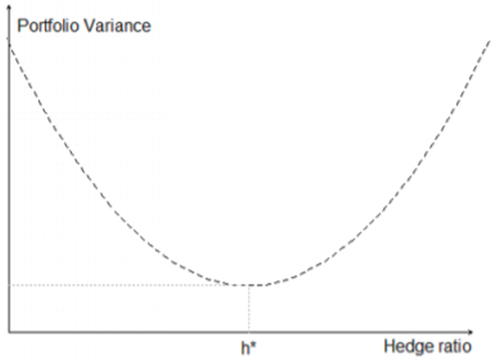
The fact that the minimum variance approach fails to distinguish hedgers both based on their interests (e.g., refiners, producers, consumers etc.), as well as on their individual investor characteristics (e.g., investors, speculators) and hence their attitude towards risk is a very important factor that needs to be taken into account, when estimating the optimal hedging ratio since hedgers may vary from the point of being reluctant to take any risk, up to the point where hedgers are found to adopt unexpectedly risky hedging strategies [47]. Figure 1 shows the graphical representation of the optimal hedging ratio.
Proper assessment of energy risk relies on models that reflect a number of important properties of the underlying assets which affect the performance of the participants’ portfolios such as time-dependent volatility and heavy tails [49]. Some of the main factors affecting hedging behavior are: profit opportunities and shareholder values which may solve conflicts over different contract preferences between companies in commodity-marketing channels [50].
3.1.1. Estimation of the Minimum-Variance hedge ratio based on the OLS methodology
The most simplistic method to estimate the Minimum-Variance hedge ratio by taking into account any potential price volatility differentials between the spot and futures prices, involves the use of the OLS regression technique between spot returns and futures returns of the examined energy portfolio [46]. Nevertheless, it is important to mention that the resulting Minimum-Variance hedge ratio of this basic analysis is static and not dynamic. Based on Equation (1) the variance of the portfolio return can be mathematically estimated as follows:
where symbolizes the portfolio’s conditional variance and the and the conditional variances of the spot and futures positions respectively, while indicates the conditional covariance.
Hence, the Minimum-Variance hedge ratio can be estimated by minimizing the portfolio’s conditional variance with respect to :
where denotes the correlation between spot and futures returns, while and represent the standard deviations.
Assuming that the variance-covariance matrix is constant and not time variant, the optimal hedge ratio can be calculated by performing an OLS regression of the spot returns on the futures returns. In this regression the slope parameter will refer to the optimal . Nevertheless, since most energy commodities are characterized by excess price volatility and thus prices are not reasonable to be considered as stationary for any reason, a dynamic analysis is required instead that will allow for a time variant optimal hedge ratio [5]. Finally, [51] point that the resulting optimal can be trustworthy only when all OLS methodology criteria are met. However, this is relatively rare to happen mostly due to the heteroskedasticity problem that econometric tests find to be present in the vast majority of energy commodity price data sets.
3.1.2. Estimation of the Minimum-Variance Hedge Ratio based on Nonlinear Multivariate Garch Models
Researchers trying to deal with the problematic and unrealistic hypothesis of the OLS approach for constant variance-covariance matrix of returns that leads to an estimation of a static optimal hedge ratio, started to implement the Arch-Garch methodology in their studies [52]. With the implementation of the appropriate Garch type volatility model (see reference [53] for a complete analysis of the econometric procedures and tests that lead to the choice of the appropriate Garch type volatility model in an energy portfolio), researchers in their estimates for the optimal hedge ratio use the conditional sample variance and covariance resulting from the chosen model.
This particular econometric technique allows for time varying variances and covariances supporting updates of the optimal hedge ratio during the hedging period. Furthermore, the Arch-Garch methodology overcomes another limitation of the OLS approach, which has to do with the presence of heteroskedasticity in the energy commodities’ data sample of price returns, as OLS regression provides unreliable and less efficient results in case of heteroskedasticity in the error term. Reference [44] suggest that the use of conditional variance and covariance in the estimation of the optimal hedge ratio for a portfolio of commodities with highly volatile returns provides significantly more accurate estimates. Additionally, [45] using a data set for six different commodities they conclude that the implementation of a static optimal hedge ratio as a hedging strategy can prove to be rather costly.
The estimation of the optimal hedge ratio even for a single energy commodity, which includes the spot and futures returns, requires the application of sophisticated nonlinear multivariate Garch models [54]. The type of volatility models are more commonly used in risk management for energy portfolios, as they are found to be superior in terms of incorporating and revealing the dynamics of variances and covariances, as well as allowing for dynamic interactions between spot and futures returns [55].
The most simplistic version of these type of models that is widely used for the estimation of the optimal hedge ratio is the VECH model, which was initially introduced by [56] and can be considered as a straightforward extension of the basic univariate GARCH model.
The VECH model is estimated as follows:
All conditional variances and covariances are functions of their own lagged values, along with lagged squared returns and cross-products of returns. Vech(.) denotes an operator, stacking the columns of the lower triangular elements of its suggested square matrix, while represents the resulting conditional covariance matrix, is an vector and are parameter matrices.
The model has the advantage of being rather simple and flexible: however it is accompanied by some serious drawbacks and limitations. That is because, firstly, as necessarily remains positive for all εt, in order to reasonably estimate all the parameters that are specified by the model, this can be diffic ult to investigate. Secondly, the large number of required parameters, as well as the demanding computational time, critically limit the model given the difficulty to consider more than two basic factors. As a result it is limited to a bivariate model [53].
According to [45] the Minimum-Variance hedge ratio in a bivariate VECH model is estimated as follows:
Let denote a (2 × 1) vector containing cash and futures prices:
With:
Considering Equation (1) the optimal hedge ratio at time t is given by:
where corresponds to the value of the exact same position in the conditional covariance matrix.
Despite its drawbacks and limitations the VECH model remains popular in estimating the Minimum-Variance hedge ratio in portfolios with a very small number of assets as it provides a time variant optimal hedge ratio rather than a single static one for the total hedging period [55].
However, in the vast majority of studies related to risk management and hedging in energy portfolios more sophisticated and complex multivariate Garch models are being used, such as the constant correlations (CCC) model and the dynamic conditional correlation model (DCC) model [53]. This is merely happening due to the advantages that these models offer to researchers compared to VECH model. Nevertheless, the more popular of the two models is [57] DCC model, which allows for a more realistic time-varying correlation structure enabling the model to capture any interactions between portfolio’s assets. As a result, the DCC model has been used recently in a larger series of studies such as [58,59,60,61,62].
The Minimum-Variance hedge ratio based on the dynamic conditional correlation model (DCC) is estimated as follows:
and:
where is the existing data set at time represents the diagonal matrix of conditional volatility with denoting the conditional variances that can be calculated using the basic Garch model and the dynamic conditional correlation.Let and the returns on the spot and futures position respectively, the following two equation provide the relative conditional variances:
While (9) with respect to becomes:
where the conditional covariance matrix is estimated as follows:
symbolizes the unconditional correlation coefficient and the standardized residuals of the spot and futures returns, respectively.
Hence the time variant Minimum-Variance hedge ratio is given by:
where denotes the conditional covariance between the spot and futures returns, and the conditional variance of futures returns.
3.2. Hedging via the Expected Utility Maximization Methodology
The maximization of the expected utility constitutes the alternative hedging approach to Minimum-Variance hedge ratio. In expected utility maximization methodology the hedger’s attitude towards risk is explicitly taken into consideration instead of assuming infinite risk aversion, by which it is implied that investors would reject investments that offer significantly high potential returns for even a relatively small additional risk [63]. This hypothesis is reasonably considered as irrational for the vast majority of hedgers, constituting risk aversion a critical factor for every risk management analysis and for the estimation of the optimal hedge ratio.
Furthermore, in contrast with Minimum-Variance hedge ratio the expected utility maximization methodology also examines the parameter of the expected return, combining elements of both risk and expected return in its estimates for the optimal hedge ratio. Nevertheless, the implementation of the risk aversion aspect requires the use of the appropriate utility function that would ideally match with the hedger’s risk preference [5]. Reference [64] analyzed data for a number of energy commodities and reported that the presence of excess skewness and kurtosis in the return distribution lead to important differentiations in the resulting optimal hedge ratios that where estimated based on specific applied utility functions.
As a result, specifying the appropriate utility function becomes a critical matter considering that these statistical characteristics are found to be present in almost every risk management analysis regarding energy commodities, while they appear to be more intense during periods of economic turmoil [64]. Specifically, large movements of certain commodities are noticed during severe crisis such as for the prices of oil [65]. Finally, another parameter of great importance that needs to be taken into account is the time variance in the hedger’s risk attitude. Table 1 shows the volatility under normal and crisis market conditions for a few commodities.
Similarly to evidence coming from financial markets, which is an even less volatile market compared to energy market, investors tend to adjust their risk preferences over time. Perhaps the most characteristic example is the 2007 economic crisis, during which investors’ perception towards risk was found to have changed dramatically. Hence, applying arbitrary risk aversion values to a hedging strategy analysis for an energy portfolio is a practice that can lead to suboptimal hedge ratios [61].
The utility concept was first introduced by Georgescu-Roegen [66,67] to explain economic values. Though since then, it has now become an obsolete concept since nobody has been able to provide a specific measurement [68]. One business model in the evolving energy sector is the energy service utility model that, unlike conventional investor-owned energy utilities, provides services such as hot water, clean electricity, or sustainable materials rather than commodities like kilowatt-hours, therms, and so on [69].
Additionally, the current business model of the utility industry is based on increasing sales and needs to be revised as electricity consumption continues to decline, at the same time energy efficiency should be a main function of the utility business model in order to reduce carbon emissions while maintaining the long-term stability of the industry [70]. More efficient distribution utility models can be designed taking into account forward looking strategies, regulatory tools, financial incentives, performance incentives and incentives for long term innovation [71].
3.2.1. Measuring Risk Aversion
Determining the degree of risk aversion has always been a challenge for researchers, nevertheless there are two measures that are more commonly used by the vast majority of researchers in the field of hedging and energy economics, consisting of the coefficients of absolute and relative risk aversion [61]. In general, the term risk aversion is basically defined as the investor’s assessment regarding the tradeoff between in taking risk that needs to be accepted for potential future return coming from the particular investment. This relationship is depicted by the investor’s utility function and the relative risk aversion is approximated by the slope change that is observed between each individual point in the function [64].
The coefficient of absolute risk aversion (CARA) examines the percentage changes of the investor’s portfolio that is invested in the risky and the risk free asset respectively regardless of the investor’s wealth level and it is mathematically described as follows:
From the above equation it is evident that an investor with CARA in absolute terms will invest a smaller part of the total portfolio value in the risky asset as wealth (W) increases.
On the contrary, the coefficient of relative risk aversion (CRRA) investigates percentage changes in the part of the investor’s portfolio that is invested in risky and risk free asset respectively, given specific changes in wealth and it is mathematically described as follows:
The above equation allows for the investor’s risk aversion to be expressed numerically, while a scale factor is used to represent the investor’s present wealth level. Nevertheless, the whole concept of the CRRA relies on the market risk premium, showing the demanded excess return by the investor’s side in order to be compensated for the additionally accepted systematic risk.
3.2.2. Optimal Hedge Ratio Estimation based on Expected Utility Theory
Assuming that and represent the expected return and variance of the hedged portfolio then the expected utility function is mathematically described as follows:
where denotes the risk aversion parameter. As a result, the hedger’s expected utility maximization is given by:
Hence the optimal hedge ratio based on the investor’s expected utility maximization can be estimated as follows:
From the above equation it is evident that in case of absolute risk aversion or the futures expected return is zero (i.e., futures prices follow a martingale), the speculative term of the equation becomes zero and as a result the estimated optimal hedge ratio becomes equivalent to the Minimum-Variance hedge ratio [6].
3.3. Alternative Hedging Strategies
Although the vast majority of academic researches incorporate primarily the Minimum-Variance methodology to estimate the optimal hedge ratio and ultimately build the most effective hedging strategy for a particular energy portfolio, there are also other approaches that aim to solve the same problem through a different perspective. The most characteristic example is the mean-risk hedge ratios, in which the optimal hedge ratios are estimated by maximizing the utility function or a specific objective function of the expected return [6]. In this alternative methodology there are three main derivations regarding risk measurement including the Sharp hedge ratio, the mean-extended-Gini (MEG) coefficient hedge ratio and the generalized semi-variance (GSV) hedge ratio.
The Sharp hedge ratio introduced by [72] actually comprises a tradeoff between risk and return, including the element of portfolio return into the hedging strategy. The Sharp hedge ratio is derived by maximizing the portfolio’s excess return relative to the portfolio’s volatility and can be calculated using the following function:
where, denotes the risk-free rate and is equal to the portfolio variance Var The Sharp hedge ratio in case the futures contracts return follows a pure martingale, it becomes equal to the optimal hedge ratio estimated by the Minimum-Variance hedge ratio.
Similarly, the MEG coefficient as proposed by [73,74,75] is estimated by minimizing the following equation:
where G represents the cumulative probability distribution.
While alternatively [76] suggest maximizing the utility function below:
In this case the estimated hedge ratio is called M-MEG and it differs from MEG hedge ratio, as it incorporates the expected return parameter into the developing hedging strategy. The two hedge ratios become equivalent when the expected return is zero (i.e., the futures returns follow a martingale). Additionally, [77] proved that the MEG hedge ratio reduces to the Minimum-Variance hedge ratio whenever the assumption that both spot and futures returns are normally distributed is confirmed. Furthermore, [73,76] show that for low values of the risk aversion parameter the MEG hedge ratio converges to Minimum-Variance hedge ratio, while significantly differentiating for increased risk aversion. Contrary, in case of high levels of risk aversion the M-MEG hedge ratio was found to become equivalent to the Minimum-Variance hedge ratio.
The third alternative mean-risk ratio is the GSV hedge ratio, which was developed by [78,79,80] and further extended by [81]. The optimal hedge ratio is estimated by minimizing the following GSV equation:
where represents the probability distribution of the hedged portfolio’s return while γ denotes the portfolio’s target return. In equation (23) it is assumed that investors consider lower than the targeted returns to be riskier, meaning that risk is measured based on a lower part of the hedged portfolio’s distribution. [79] verify that the GSV hedge ratio becomes equivalent to the Minimum-Variance hedge ratio, provided that both assumptions for joint normality in the return distribution and pure martingale price process are met.
Extending the abovementioned hedge ratio methodology, [81] alter the GSV hedge ratio by including the mean return parameter in the derivation of the optimal hedge ratio. In this case, the produced mean-GSV hedge ratio is estimated by maximizing the below utility function:
Reference [81] show that the M-GSV hedge ratio would become equivalent to the Minimum-Variance hedge ratio if both the pure martingale and joint normality hypotheses hold. Reference [80] suggest that adopting a conventional Minimum-Variance hedge strategy is unsuitable for hedgers that are mostly worried about downside risk. As a result, because of its conceptual simplicity for measuring the downside risk of a hedged portfolio the VaR methodology is being adopted by researchers as an alternative approach to build the optimal hedging strategy. Such case is the VaR constraint approach, which involves estimating the optimal hedge ratio based on a certain acceptable amount of risk or expected profit. Reference [82] where the first to build a VaR constraint hedging optimization model motivated by the high level of risk in the US electricity, with [83] following.
4. State of the Art—Relevant Studies Using Hedging Strategies
Although the specific research field in general became popular only recently, there is a number of very interesting research papers trying to explore the most important aspects for employing a successful hedging strategy regarding energy commodities, which are further presented in this Section.
4.1. Optimal Hedging Strategies based on the Minimum Variance Methodology
The Minimum-Variance hedge ratio methodology, despite its demerits, is by far the most widely used in academic literature offering useful advice about the mixture of the hedging strategy that should be employed by a firm that is exposed to energy price risk [5]. Therefore, many researchers use the Minimum-Variance hedge ratio to provide guidance to risk managers relative to the most appropriate hedging policy that would lead to reduced stock price volatility and increased firm value.
Reference [84] are some of the first that focused on estimating the most suitable hedging ratios regarding the crude oil market. The authors were using a four-year weekly spot price data sample for crude oil futures and the basic ARCH and GARCH models, and they concluded that the optimal hedging ratio is time-varying and that is positively affected by the duration of the contracts. Next, [61] using a much larger sample of daily spot prices for both Brent and WTI oil from a period from 1997 to 2009, tested several multivariate volatility models for their ability to estimate the most effective optimal hedge ratio, determining that the diagonal BEKK model is the most appropriate. Furthermore, they suggested a hedging strategy which involves an increased proportion of shorting in crude oil futures.
Reference [85] while emphasizing on the oil refining industry, they examine the weekly spot and futures prices for a 15-year period (1994–2009), regarding three of the most important and characteristic energy products in that specific industry, including the WTI crude oil, heating oil and gasoline. Their empirical results reveal that a combination of a dynamic conditional correlation (DCC) model and error correction GARCH model is better compared to simplified GARCH based models to capture the risk for refiners stemming both from the crude oil market itself, as well as the oil product market.
Finally, [86] were the first to examine the natural gas market and build an optimal hedging strategy using a single Henry-Hub futures contract. Specifically, they reveal that an adjusted error correction GARCH model is by far more capable of estimating the most effective time-varying hedging ratio relative to the conventional OLS methodology and several basic GARCH models. Moreover, based on the results of their research it is also supported that taking into consideration the elements of co-integration and time varying volatility doesn’t have a significant impact on the hedging effectiveness of a specific strategy.
4.2. Incorporating the Elements of Risk Aversion and Expected Return into the Optimal Hedging Strategy
A rather interesting factor, when investigating the hedging policies of particular industries, is the tendency as well as the willingness of the market participants to take risks. The risk attitude of an industrial firm, which is exposed to the energy price risk may seriously affect the overall hedging policy of the firm regarding energy products considering their increased price volatility [37].
Although the above issue constitutes a quite interesting topic for further research, the fact that incorporating a risk aversion factor in such a study can prove to be tricky, as well as computationally demanding and time consuming, probably discouraged most academics to deal with the aforementioned topic. Specifically, [64] are the first who try to address the problem of risk aversion incorporation in an optimal hedging strategy regarding energy products.
The researchers while applying a GARCH in Mean model, estimate the optimal hedging ratio relying on a sample for gasoline futures prices for a 16-year period between 1992 and 2008. However, the innovative element of their study, is that in their model’s estimates a time varying risk aversion factor is taken into consideration, enabling them to forecast risk aversion and thus better adjust the hedging strategy to the hedger’s future needs. Finally, [87] further extend the previous study by incorporating the factor of risk aversion to the most popular and frequently applied utility functions and through that they end up to the most appropriate and efficient hedging strategy.
5. Conclusions
Energy is considered as a commodity nowadays and continuous access along with price stability is of vital importance for every economic agent worldwide. The current study comprehensively reviews the advantages and disadvantages of the main hedging methodologies regarding risk management in energy portfolios. Additionally, it enables the reader to explain, analyze and interpret the variations in the results for the proposed optimal hedging strategies of each methodology, while advising when and why choosing a specific methodology over the others and if more than one methodology is required to build a more reliable hedging strategy due to special economic characteristics of a certain time period.
Based on the conducted review, it is clear that the Minimum-Variance hedge ratio methodology if the appropriate nonlinear multivariate model is used, the Garch family volatility model can provide a reliable optimal hedge ratio with relatively low computational effort. However, that becomes possible by applying a rather restrictive assumption for infinite risk aversion on behalf of the investor into the analysis. This estimation gap of an optimal hedge ratio that would be subject to the investor’s risk preferences through time is filled by the relatively more complex and sophisticated expected utility maximization methodology. Nevertheless, if hedgers share infinite risk aversion or if alternatively the expected futures price variation is approximately zero, the two methodologies become equivalent.
In general, considering evidence from the energy market the assumption that energy futures prices follow a martingale is confirmed for extended periods of time, yet during periods with extremely volatile economic climate and financial crisis this may change until the market returns to normality. Finally, it is important to note that during periods of extreme uncertainty and high risk it is common also for the investors’ risk attitude to show significant variations. Hence, it becomes reasonable that especially for extended hedging horizons it would be wise for potential hedgers to take into consideration both methodologies in order to build a successful and profitable hedging strategy.
A numerical analysis is proposed as a further extension of the present paper, in which the resulting hedging strategies from the different methodologies would be tested regarding their effectiveness and profitability through multiple time horizons and for several energy commodities. An important limitation of this research has to do with resources decoupling and keeping under control the increasing of the value added and decreasing energy consumption.
Author Contributions
G.E.H. conceived and designed the analysis. Both G.E.H. and A.S.T. wrote the manuscript and contributed to the final version of the manuscript. G.E.H. supervised the paper, provided critical feedback and helped shape the research.
Funding
This research received no external funding.
Acknowledgments
We would like to thank the Editor and the three anonymous reviewers for the helpful and constructive comments on earlier drafts of our paper. Any remaining errors are solely the authors’ responsibility.
Conflicts of Interest
The authors declare no conflicts of interest
References
- European Commission. Study on Energy Efficiency and Energy Saving Potential in Industry and on Possible Policy Mechanism; EC: Brussels, Belgium, 2015. [Google Scholar]
- Boroumand, R.H.; Goutte, S.; Porcher, S.; Porcher, T. Hedging strategies in energy markets: The case of electricity retailers. Energy Econ. 2015, 51, 503–509. [Google Scholar] [CrossRef]
- Zhang, J.; Tan, K.S.; Weng, C. Optimal hedging with basis risk under mean–variance criterion. Insur. Math. Econ. 2017, 75, 1–15. [Google Scholar] [CrossRef]
- Stulz, R.M. Optimal Hedging Policies. J. Financ. Quant. Anal. 1984, 19, 127–140. [Google Scholar] [CrossRef]
- Dewally, M.; Marriott, L. Effective Basemetal Hedging: The Optimal Hedge Ratio and Hedging Horizon. J. Risk Financ. Manag. 2008, 1, 41–76. [Google Scholar] [CrossRef]
- Hung, J.-C.; Chiu, C.-L.; Lee, M.-C. Hedging with zero-value at risk hedge ratio. Appl. Financ. Econ. 2006, 16, 259–269. [Google Scholar] [CrossRef]
- Halkos, G.E.; Tsirivis, A.S. Value-at-risk methodologies for effective energy portfolio risk management. Econ. Anal. Policy 2019, 62, 197–212. [Google Scholar] [CrossRef]
- Ricardo, D. On the Principles of Political Economy and Taxation; John Murray: London, UK, 1817. [Google Scholar]
- Manoilescu, M. Die Nationalen Producktivkräfte und der Aussenhandel. Theorie des Internationalen Warenaustausches, Junker und Dünnhaupt, Name? Juncker & Dünnhaupt: Berlin, Germany, 1937. [Google Scholar]
- Balassa, B. Trade Liberalisation and “Revealed” Comparative Advantage. Manch. Sch. 1965, 33, 99–123. [Google Scholar] [CrossRef]
- Porter, M.E. The Comparative Advantage of Nations. Harv. Bus. Rev. 1990, 73–91. [Google Scholar] [CrossRef]
- Dogaru, V. The expanding of constructal law in economics—A justification for crossed flows of similar macro goods. Int. J. Heat Technol. 2016, 34, 59–74. [Google Scholar] [CrossRef]
- Kuik, O.; Branger, F.; Quirion, P. Competitive advantage in the renewable energy industry: Evidence from a gravity model. Renew. Energy 2019, 131, 472–481. [Google Scholar] [CrossRef]
- Blum, J. Energy Bankruptcies Back on the Rise in 2019; Houston Chronicle: Houston, TA, USA, 2019. [Google Scholar]
- Seba, E. Bankruptcy Filings by U.S. Energy Producers Pick up Speed: Law Firm Analysis; Reuters: London, UK, 2019. [Google Scholar]
- Haushalter, G.D. Financing Policy, Basis Risk, and Corporate Hedging: Evidence from Oil and Gas Producers. J. Financ. 2000, 55, 107–152. [Google Scholar] [CrossRef]
- Haushalter, G.D. Why Hedge? Some Evidence from Oil and Gas Producers. J. Appl. Corp. Financ. 2001, 13, 87–92. [Google Scholar] [CrossRef]
- Chew, D. Energy Derivatives and the Transformation of the U.S. Corporate Energy Sector. J. Appl. Corp. Financ. 2001, 13, 50–75. [Google Scholar]
- Smithson, C.; Simkins, B.J. Does Risk Management Add Value? A Survey of the Evidence. J. Appl. Corp. Finance 2005, 17, 8–17. [Google Scholar] [CrossRef]
- Carter, D.A.; Rogers, D.A.; Simkins, B.J. Does Hedging Affect Firm Value? Evidence from the US Airline Industry. Financ. Manag. 2006, 35, 53–86. [Google Scholar] [CrossRef]
- Geczy, C.; Minton, B.; Schrand, C. Choices among Alternative Risk Management Strategies: Evidence from the Natural Gas Industry; Working Paper Wharton School of Economics; The Rodney L. White Center for Financial Research: Pennsylvania, PA, USA, 2002. [Google Scholar]
- Jin, Y.; Jorion, P. Firm Value and Hedging: Evidence from U.S. Oil and Gas Producers. J. Financ. 2006, 61, 893–919. [Google Scholar] [CrossRef]
- Islam, M.; Chakraborti, J. Futures and forward contract as a route of hedging the risk. Risk Gov. Control. Financ. Mark. Inst. 2015, 5, 68–78. [Google Scholar] [CrossRef]
- Trafigura. Commodities Demystified: A Guide to Trading and the Global Supply Chain 2018. Available online: www.trafigura.com (accessed on 10 July 2019).
- Difiglio, C. Oil, economic growth and strategic petroleum stocks. Energy Strat. Rev. 2014, 5, 48–58. [Google Scholar] [CrossRef] [Green Version]
- Economic Consulting Associates Limited. European Electricity: Forward Markets and Hedging Products—State of Play and Elements for Monitoring 2015. Available online: www.acer.europa.eu (accessed on 10 July 2019).
- Malik, F. Risk Management: Understanding Credit Risk. Available online: www.medium.com (accessed on 10 July 2019).
- Mas, I.; Saa-Requejo, J. Using Financial Futures in Trading and Risk Management; Policy Research Working Paper; World Bank: Washington, DC, USA, 1995. [Google Scholar]
- IOSCO. Report on the International Regulation of Derivative Markets, Products and Financial Intermediaries 2012. Available online: www.trafigura.com (accessed on 15 July 2019).
- Carmona, R.; Durrleman, V. Pricing and Hedging Spread Options. SIAM Rev. 2003, 45, 627–685. [Google Scholar] [CrossRef] [Green Version]
- New York Mercantile Exchange. A guide to Energy Hedging. Available online: www.renesource.com (accessed on 5 July 2019).
- Coffman, D.; Lockley, A. Carbon dioxide removal and the futures market. Environ. Res. Lett. 2017, 12, 015003. [Google Scholar] [CrossRef]
- Keytrade Bank. Options Manual of Keytrade Bank; Keytrade Bank: Brussels, Belgium, 2017. [Google Scholar]
- Mercatus. An Introduction to Crack Spread (Refiner) Hedging 2019. Available online: www.mercatusenergy.com (accessed on 30 July 2019).
- Vitale, L. Interest Rate Swaps under the Commodity Exchange Act. Case West. Reserve Law Rev. 2001, 51, 539–591. [Google Scholar]
- Ernst & Young. Financial Reporting Developments A Comprehensive Guide Derivatives and Hedging. Available online: www.ey.com (accessed on 25 July 2019).
- Deloitte. Commodity Price Risk Management: A manual of Hedging Commodity Price Risk for Corporates 2018. Available online: www2.deloitte.com (accessed on 16 July 2019).
- Stoft, S.; Belden, T.; Goldman, C.; Pickle, S. Primer on Electricity Futures and Other Derivatives; Environmental Energy Technologies Division, Ernest Orlando Lawrence Berkeley National Laboratory, University of California Berkeley: Berkeley, CA, USA, 1998. [Google Scholar]
- Devlin, J.; Titman, S. Managing Oil Price Risk in Developing Countries. World Bank Res. Obs. 2004, 19, 119–139. [Google Scholar] [CrossRef] [Green Version]
- Ritchken, P. Hedging with Futures Contracts. Case West-ern Reserve University—Class Notes 1999. Available online: http://faculty.weatherhead.case.edu (accessed on 5 July 2019).
- Castellino, M.G. Hedge effectiveness: Basis risk and minimum-variance hedging. J. Futures Mark. 2000, 20, 89–103. [Google Scholar] [CrossRef]
- Johnson, L.L. The Theory of Hedging and Speculation in Commodity Futures. Rev. Econ. Stud. 1960, 27, 139. [Google Scholar] [CrossRef]
- Ederington, L.H. The Hedging Performance of the New Futures Markets. J. Financ. 1979, 34, 157–170. [Google Scholar] [CrossRef]
- Myers, R.J.; Thompson, S.R. Generalized Optimal Hedge Ratio Estimation. Am. J. Agric. Econ. 1989, 71, 858–868. [Google Scholar] [CrossRef] [Green Version]
- Baillie, R.T.; Myers, R.J. Bivariate garch estimation of the optimal commodity futures Hedge. J. Appl. Econ. 1991, 6, 109–124. [Google Scholar] [CrossRef]
- Yu, H. The Implication of Currency Hedging Strategies for Pension Funds. Master’s Thesis, MSc Finance—Pension Track Tilburg University, Tilburg, The Netherlands, 2014. [Google Scholar]
- Arthur, J.N.; Williams, R.J.; Delfabbro, P.H. The conceptual and empirical relationship between gambling, investing, and speculation. J. Behav. Addict. 2016, 5, 580–591. [Google Scholar] [CrossRef] [Green Version]
- Benada, L. Hedging of Energy Commodities. Ph.D. Thesis, Masaryk University, Brno, Czech Republic, 2017. [Google Scholar]
- Pouliasis, P. Essays on the Empirical Analysis of Energy Risk. Ph.D. Thesis, Cass Business School, London, UK, 2011. [Google Scholar]
- Pennings, J.M.E. What Drives Actual Hedging Behaviour? Developing Risk Management Instruments. In Agribusiness and Commodity Risk: Strategies and Management; Risk Books: London, UK, 2003; pp. 63–74. [Google Scholar]
- Chen, S.S.; Lee, C.; Shrestha, K. Futures hedge ratios: A review. Quart. Rev. Econ. Financ. 2003, 43, 433–465. [Google Scholar] [CrossRef]
- Harris, R.D.F.; Stoja, E.; Tucker, J. A Simplified Approach to Modelling the Comovement of Asset Returns. J. Futures Mark. 2007, 27, 575–598. [Google Scholar] [CrossRef]
- Halkos, G.E.; Tsirivis, A.S. Effective energy commodity risk management: Econometric modeling of price volatility. Econ. Anal. Pol. 2019, 63, 234–250. [Google Scholar] [CrossRef]
- Alizadeh, A.H.; Nomikos, N.K.; Pouliasis, P.K. A Markov regime switching approach for hedging energy commodities. J. Bank. Financ. 2008, 32, 1970–1983. [Google Scholar] [CrossRef]
- Casillo, A. Model Specification for the Estimation of the Optimal Hedge Ratio with Stock Index Futures: An Application to the Italian Derivatives Market. Available online: www.luiss.it (accessed on 18 October 2019).
- Bollerslev, T.; Engle, R.F.; Wooldridge, J.M. A Capital Asset Pricing Model with Time-Varying Covariances. J. Polit. Econ. 1988, 96, 116–131. [Google Scholar] [CrossRef]
- Engle, R.F. Dynamic Conditional Correlation: A Simple Class of Multivariate Generalized Autoregressive Conditional Heteroskedasticity Models. J. Bus. Econ. Stat. 2002, 20, 339–350. [Google Scholar] [CrossRef]
- Manera, M.; McAleer, M.; Grasso, M. Modelling time-varying conditional correlations in the volatility of Tapis oil spot and forward returns. Appl. Financ. Econ. 2006, 16, 525–533. [Google Scholar] [CrossRef]
- Liu, S.D.; Jian, J.B.; Wang, Y.Y. Optimal dynamic hedging of electricity futures based on copula-GARCH models. In Proceedings of the 2010 IEEE International Conference on Industrial Engineering and Engineering Management, Macao, China, 7–10 December 2010; pp. 2498–2502. [Google Scholar]
- Zanotti, G.; Gabbi, G.; Geranio, M. Hedging with futures: Efficacy of GARCH correlation models to European electricity markets. J. Int. Financ. Mark. Inst. Money 2010, 20, 135–148. [Google Scholar] [CrossRef]
- Chang, C.-L.; McAleer, M.; Tansuchat, R. Crude oil hedging strategies using dynamic multivariate GARCH. Energy Econ. 2011, 33, 912–923. [Google Scholar] [CrossRef] [Green Version]
- Basher, S.A.; Sadorsky, P. Hedging emerging market stock prices with oil, gold, VIX, and bonds: A comparison between DCC, ADCC and GO-GARCH. Energy Econ. 2016, 54, 235–247. [Google Scholar] [CrossRef] [Green Version]
- Heisler, A. 7 Critical Risks Impacting the Energy Industry. Risk & Insurance. Available online: www.riskandinsurance.com (accessed on 5 July 2019).
- Cotter, J.; Hanly, J. Time-varying risk aversion: An application to energy hedging. Energy Econ. 2010, 32, 432–441. [Google Scholar] [CrossRef] [Green Version]
- Al Janabi, M.A.M. Commodity price risk management: Valuation of large trading portfolios under adverse and illiquid market settings. J. Deriv. Hedge Funds 2009, 15, 15–50. [Google Scholar] [CrossRef] [Green Version]
- Georgescu-Roegen, N. Choice, Expectations and Measurability. Quart. J. Econ. 1954, 68, 503–534. [Google Scholar] [CrossRef]
- Georgescu-Roegen, N. Utility. Int. Encycl. Soc. Sci. 1968, 16, 236–267. [Google Scholar]
- Georgescu-Roegen, N. The Entropy Law and the Economic Process. East. Econ. J. 1971, 12. [Google Scholar]
- Byrne, J.; Taminiau, J. A review of sustainable energy utility and energy service utility concepts and applications: Realizing ecological and social sustainability with a community utility. WIREs Energy Environ. 2016, 5, 136–154. [Google Scholar] [CrossRef]
- Fox-Penner, P. The Smart Grid–Enabled Energy Services Utility: How Utilities Can Become Sustainable by Selling Less. Solutions 2010, 1, 42–48. [Google Scholar]
- MIT. Utility of the Future. 2016, An MIT Energy Initiative Response to an Industry in Transition. Available online: energy.mit.edu (accessed on 9 July 2019).
- Howard, C.T.; D’Antonio, L.J. A Risk-Return Measure of Hedging Effectiveness. J. Financ. Quant. Anal. 1984, 19, 101. [Google Scholar] [CrossRef]
- Kolb, R.W.; Okunev, J. An empirical evaluation of the extended mean-gini coefficient for futures hedging. J. Futures Mark. 1992, 12, 177–186. [Google Scholar] [CrossRef]
- Lien, D.; Luo, X. Estimating the extended mean-gini coefficient for futures hedging. J. Futures Mark. 1993, 13, 665–676. [Google Scholar] [CrossRef]
- Gregory-Allen, R.B.; Shalit, H. The Estimation of Systematic Risk under Differentiated Risk Aversion: A Mean-Extended Gini Approach. Rev. Quant. Financ. Account. 1999, 12, 135–158. [Google Scholar] [CrossRef]
- Kolb, R.W.; Okunev, J. Utility maximizing hedge ratios in the extended mean gini framework. J. Futures Mark. 1993, 13, 597–609. [Google Scholar] [CrossRef]
- Shalit, H. Mean-Gini hedging in futures markets. J. Futures Mark. 1995, 15, 617–635. [Google Scholar] [CrossRef]
- De Jong, A.; De Roon, F.; Veld, C. Out-of-sample hedging effectiveness of currency futures for alternative models and hedging strategies. J. Futures Mark. 1997, 17, 817–837. [Google Scholar] [CrossRef]
- Lien, D.; Tse, Y.K. Hedging time-varying downside risk. J. Futures Mark. 1998, 18, 705–722. [Google Scholar] [CrossRef]
- Lien, D.; Tse, Y.K. Hedging downside risk with futures contracts. Appl. Financ. Econ. 2000, 10, 163–170. [Google Scholar] [CrossRef]
- Chen, S.-S.; Lee, C.-F.; Shrestha, K. On a Mean—Generalized Semivariance Approach to Determining the Hedge Ratio. J. Futures Mark. 2001, 21, 581–598. [Google Scholar] [CrossRef]
- Kleindorfer, P.R.; Li, L. Multi-Period VaR-Constrained Portfolio Optimization with Applications to the Electric Power Sector. Energy J. 2005, 26, 1–26. [Google Scholar] [CrossRef]
- Oum, Y.; Oren, S. VaR constrained hedging of fixed price load-following obligations in competitive electricity markets. Risk Dec. Anal. 2009, 1, 43–56. [Google Scholar] [Green Version]
- Jalali-Naini, A.R.; Manesh, M.K. Price volatility, hedging and variable risk premium in the crude oil market. OPEC Rev. 2006, 30, 55–70. [Google Scholar] [CrossRef]
- Ji, Q.; Fan, Y. A dynamic hedging approach for refineries in multiproduct oil markets. Energy 2011, 36, 881–887. [Google Scholar] [CrossRef]
- Ghoddusi, H.; Emamzadehfard, S. Optimal hedging in the US natural gas market: The effect of maturity and cointegration. Energy Econ. 2017, 63, 92–105. [Google Scholar] [CrossRef]
- Cotter, J.; Hanly, J. Performance of utility based hedges. Energy Econ. 2015, 49, 718–726. [Google Scholar] [CrossRef] [Green Version]
Figure 1.
Hedge position and the shape of portfolio variance [48].
Figure 1.
Hedge position and the shape of portfolio variance [48].


Table 1.
Risk analysis data—volatility under normal and crisis market conditions and sensitivity factors (adapted from [65]).
Table 1.
Risk analysis data—volatility under normal and crisis market conditions and sensitivity factors (adapted from [65]).
| Commodity Name | Monthly Volatility (Normal Market) (%) | Monthly Volatility (Crisis Market) (%) | Annual Volatility (Normal Market) (%) | Annual Volatility (Crisis Market) (%) | Sensitivity Factors |
|---|---|---|---|---|---|
| Petroleum: average crude price | 8.1 | 24.6 | 28.1 | 85.2 | 1.72 |
| Gasoline | 10.4 | 25.4 | 30.4 | 87.2 | 1.88 |
| Natural gas | 5.8 | 20.6 | 20.0 | 71.2 | 0.14 |
| Coal | 4.0 | 13.5 | 13.9 | 46.9 | 0.26 |
| Gold | 3.3 | 12.5 | 11.3 | 43.2 | 0.18 |
| Silver | 5.4 | 21.6 | 18.7 | 75.0 | 0.18 |
| Copper | 6.2 | 20.0 | 21.5 | 69.2 | 0.48 |
| Zinc | 6.1 | 24.9 | 21.3 | 86.4 | 0.34 |
| Lead | 6.3 | 23.8 | 21.9 | 82.3 | 0.15 |
| Aluminum | 5.8 | 32.6 | 20.0 | 133.1 | 0.31 |
| Nickel | 8.9 | 22.2 | 30.7 | 76.9 | 0.54 |
| Iron ore | 4.4 | 12.9 | 15.2 | 44.7 | 0.18 |
| Phosphate rock | 2.3 | 21.7 | 8.1 | 75.2 | 0.01 |
| Wheat | 5.1 | 15.1 | 17.7 | 52.3 | 0.08 |
| Cotton | 4.9 | 12.6 | 17.0 | 43.5 | 0.14.9 |
| Sugar | 2.1 | 11.0 | 7.3 | 38.2 | −0.05 |
| Maize | 5.3 | 25.2 | 18.4 | 87.2 | −0.08 |
| Tobacco | 1.8 | 4.9 | 6.2 | 16.8 | 0.01 |
| Coffee | 8.0 | 37.1 | 27.6 | 128.6 | 0.04 |
| Tea | 7.7 | 23.6 | 26.8 | 81.8 | 0.11 |
| Rubber | 6.0 | 18.1 | 20.8 | 62.7 | 0.37 |
| Wool | 4.7 | 16.5 | 16.4 | 57.3 | −0.02 |
| All commodities | 3.6 | 12.3 | 12.5 | 42.5 | 1.00 |
© 2019 by the authors. Licensee MDPI, Basel, Switzerland. This article is an open access article distributed under the terms and conditions of the Creative Commons Attribution (CC BY) license (http://creativecommons.org/licenses/by/4.0/).
Share and Cite
MDPI and ACS Style
Halkos, G.E.; Tsirivis, A.S. Energy Commodities: A Review of Optimal Hedging Strategies. Energies 2019, 12, 3979. https://0-doi-org.brum.beds.ac.uk/10.3390/en12203979
AMA Style
Halkos GE, Tsirivis AS. Energy Commodities: A Review of Optimal Hedging Strategies. Energies. 2019; 12(20):3979. https://0-doi-org.brum.beds.ac.uk/10.3390/en12203979
Chicago/Turabian StyleHalkos, George E., and Apostolos S. Tsirivis. 2019. "Energy Commodities: A Review of Optimal Hedging Strategies" Energies 12, no. 20: 3979. https://0-doi-org.brum.beds.ac.uk/10.3390/en12203979
Note that from the first issue of 2016, this journal uses article numbers instead of page numbers. See further details here.