Fuzzy Logic Control for Low-Voltage Ride-Through Single-Phase Grid-Connected PV Inverter

Abstract

This paper presents a control scheme for a photovoltaic (PV) system that uses a single-phase grid-connected inverter with low-voltage ride-through (LVRT) capability. In this scheme, two PI regulators are used to adjust the power angle and voltage modulation index of the inverter; therefore, controlling the inverter’s active and reactive output power, respectively. A fuzzy logic controller (FLC) is also implemented to manage the inverter’s operation during the LVRT operation. The FLC adjusts (or de-rates) the inverter’s reference active and reactive power commands based on the grid voltage sag and the power available from the PV system. Therefore, the inverter operation has been divided into two modes: (i) Maximum power point tracking (MPPT) during the normal operating conditions of the grid, and (ii) LVRT support when the grid is operating under faulty conditions. In the LVRT mode, the de-rating of the inverter active output power allows for injection of some reactive power, hence providing voltage support to the grid and enhancing the utilization factor of the inverter’s capacity. The proposed system was modelled and simulated using MATLAB Simulink. The simulation results showed good system performance in response to changes in reference power command, and in adjusting the amount of active and reactive power injected into the grid.

1. Introduction

Distributed generation (DG) systems are gaining global interest as a result of environmental concerns, increase in fuel cost, political reasons, and economic impact. Renewable energy sources accounted for 17.5% of the global energy consumption in 2016 [1]. Among the various DG systems, solar PV energy is considered one of the most popular renewable energy sources. It is a clean form of energy, inexhaustible, requires little maintenance, offers flexibility of installation, and its cost is decreasing [2,3]. Solar PV generation increased 31% in 2018 and represented the largest absolute generation growth (+136 TWh) of all renewable technologies, slightly ahead of wind and hydropower [4]. For power output below 10 kW; single-phase voltage source inverter (VSI) configuration is found to be one of the preferable methods for interfacing and integrating small ratings PV system to the grid [5,6,7].

Although the integration of single-phase PV systems with the grid has its advantages, the widespread use of PV systems poses more challenging issues for distribution system operators and the entire grid [8]. One of the important drawbacks of a grid-tied PV system is the existence of an inverter as interface between the PV system and the grid. This leads to many problems: safety, efficiency, stability (voltage and frequency), increased level of harmonics, and poor power factor of the entire system [9,10]. To minimize the effects of grid-connected PV systems, specific grid requirements regarding the penetration of grid-connected PV systems in low voltage networks have been put forward, as outlined in the EN 50160 and IEEE1547 standards. These standards specify that grid-connected PV systems must comply with levels of total harmonic distortion (THD), power factor, level of injected DC current, and voltage and frequency range [2,8].

One of the emergent grid requirements that has become the focus of recent research topics, and has been gaining increased attention is the low-voltage ride-through (LVRT) capability of solar PV systems [11,12,13,14,15]. The LVRT capability of a PV system requires the DG systems to remain connected to the grid during grid faults (e.g., voltage sag), and to supply reactive power to support the grid. Smart management and control of inverter-PV systems characterized by the capability of the inverter to operate over a range of voltages, inject reactive power, and provide other ancillary services to the grid is becoming a requirement grid-code in many countries, such as Denmark, Germany, UK, Canada, Ireland, and Spain [16].

Researchers discussed the LVRT capability of single-phase and three-phase grid-connected PV systems in recent studies [8,12,13,14,15,17]. The control of single-phase grid-connected systems with reactive power injection can be achieved through many different methods, e.g., direct power control, droop concept, and single-phase PQ theory [8,15]. The latter method is less complex, but requires an orthogonal signal generator (OSG) unit to produce orthogonal signal components. In [12], a dynamic voltage restorer based on FLC was used to compensate for the voltage drop during the voltage sags. The proposed method required a voltage source converter, injection transformer, energy storage devices, and other ancillaries. This leads to a less economic and more expensive solution when considering low power single-phase systems. Moreover, [15] simulated the functionalities of LVRT and validated it experimentally using conventional control techniques. Also, [18] proposed complete control technique of single-stage PV power plant in order to support LVRT ability. The proposed technique is based on local Malaysian standards and using up-to-date grid connection instruction and requirements, mainly DC-chopper brake controller and current limiter, which limits DC over-voltage and AC over current. It is worth mentioning here that [19] investigated a control technique which relies on using Fuzzy-Proportional Integral controller in order to control inner current control loop, and the outer power control loop, thus enhancing current injection to the grid. In the literature, [20] proposed a new design using proportional resonant controller (PRC) alongside a resonant-harmonic corrector and switch-type fault current limiter, for a three-phase, grid-connected solar PV system under regular situation and symmetric faults.

This paper presents a simulation study of a single-stage, single-phase grid-connected inverter using MATLAB Simulink. Active and reactive power output from the inverter were controlled using the power angle and voltage modulation index of the inverter, respectively. A FLC was used to determine the amount of active and reactive power to be injected into the grid. The voltage at the point of common coupling (PCC) in the DQ reference frame, and the amount of real power available from the PV system are used by the FLC to calculate power factor (PF) at which power is injected into the grid. The uniqueness of the proposed system is the use of a FLC to estimate how much reactive power is to be injected into the system by recommending a PF value. The PF value is then used to calculate the reactive power using the full capacity of the inverter, without de-rating the active power. The active and reactive power calculator (PQ) uses the initially estimated reference real power ($P^{*}$) and reactive power ($Q^{*}$) and ensures that inverter ratings are not exceeded (the maximum current). If the maximum current is exceeded, real power is de-rated using the recommended PF value. Both reference commands are used by the respective PI controllers to adjust the power angle ($\delta$) and the voltage modulation index ($\Delta v_i$) of the inverter. Simulation results showed that the proposed control strategy of the inverter system responded satisfactorily during the maximum power point tracking (MPPT) and LVRT modes of operation.

The work presented in this paper is organized as follows: Section 2 presents the theoretical background of the proposed system and its main blocks. Section 3 presents the simulation results (using Simulink/MATLAB) of the system under investigation. The conclusion of the system performance is presented in Section 4.

2. System Structure and Proposed Control Methods

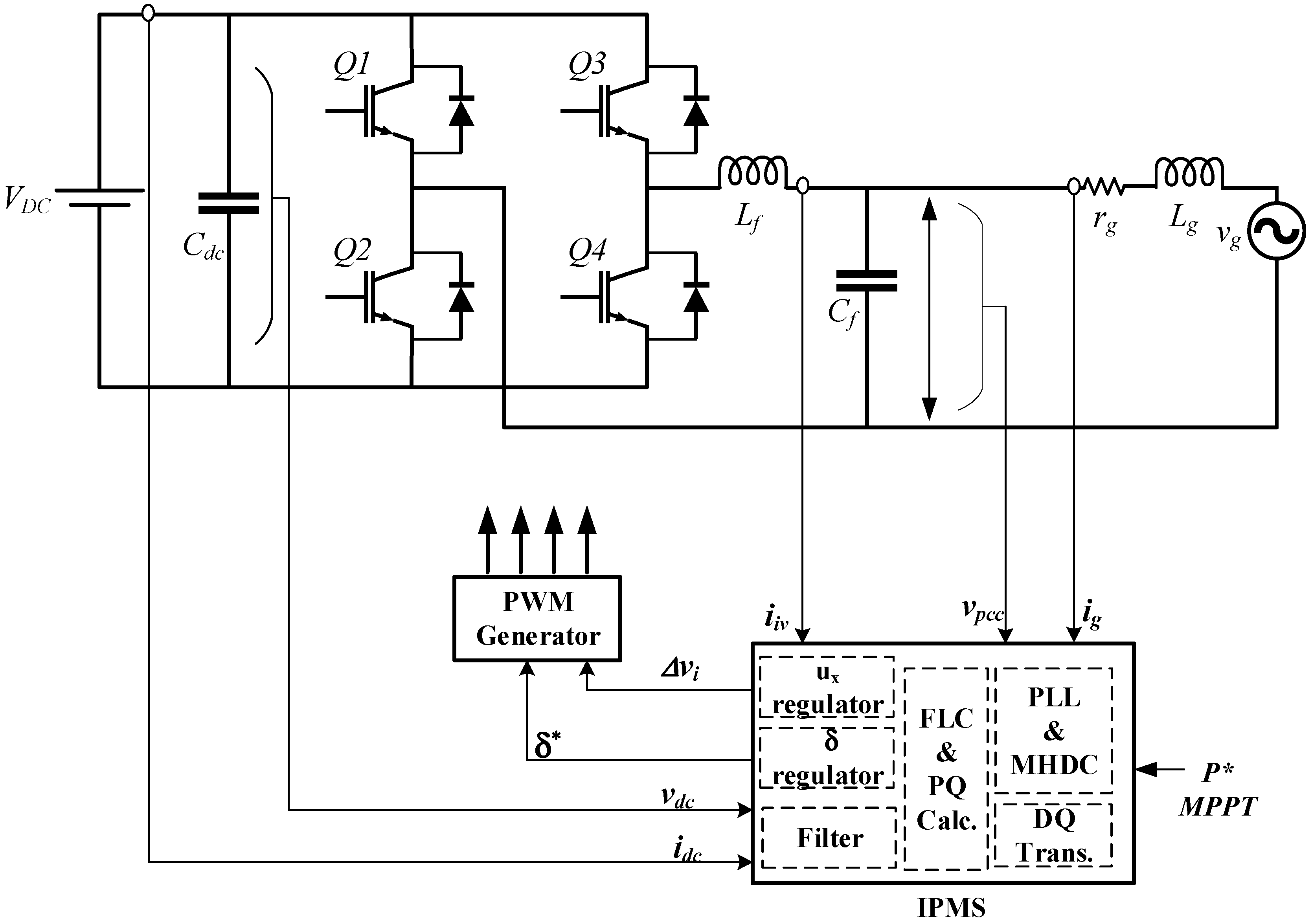
Figure 1 shows the block diagram of the system presented in this research work. The single-phase inverter in Figure 1 operates with unipolar PWM switching strategy, and is supplied from a constant DC voltage source that emulates the output from a boost DC converter. An LC filter is connected between the inverter and the utility grid equivalent model to maintain total harmonic distortion within acceptable limits. The measured signals that are required in the proposed control scheme are shown as inputs to inverter power management system (IPMS). The role of the IPMS unit is to operate on the measured signals and perform the required calculations to determine the commanded power angle and voltage modulation index to be used in controlling the inverter. A more detailed explanation about the building blocks of the IPMS is given in the following subsections.

2.1. PLL and MHDC

The phase locked loop (PLL) and multiple-harmonic decoupling cell (MHDC) are implemented to estimate the phase angle of the grid and filter the higher order components in the measured signals, respectively. The design details of the PLL and MHDC units can be obtained from the work presented in [21,22]. The output from these units is used to transform the measured voltage and current signals to the DQ reference frame to facilitate operating on them in a manner similar to DC signals.

2.2. Fuzzy Logic and PQ Calculator

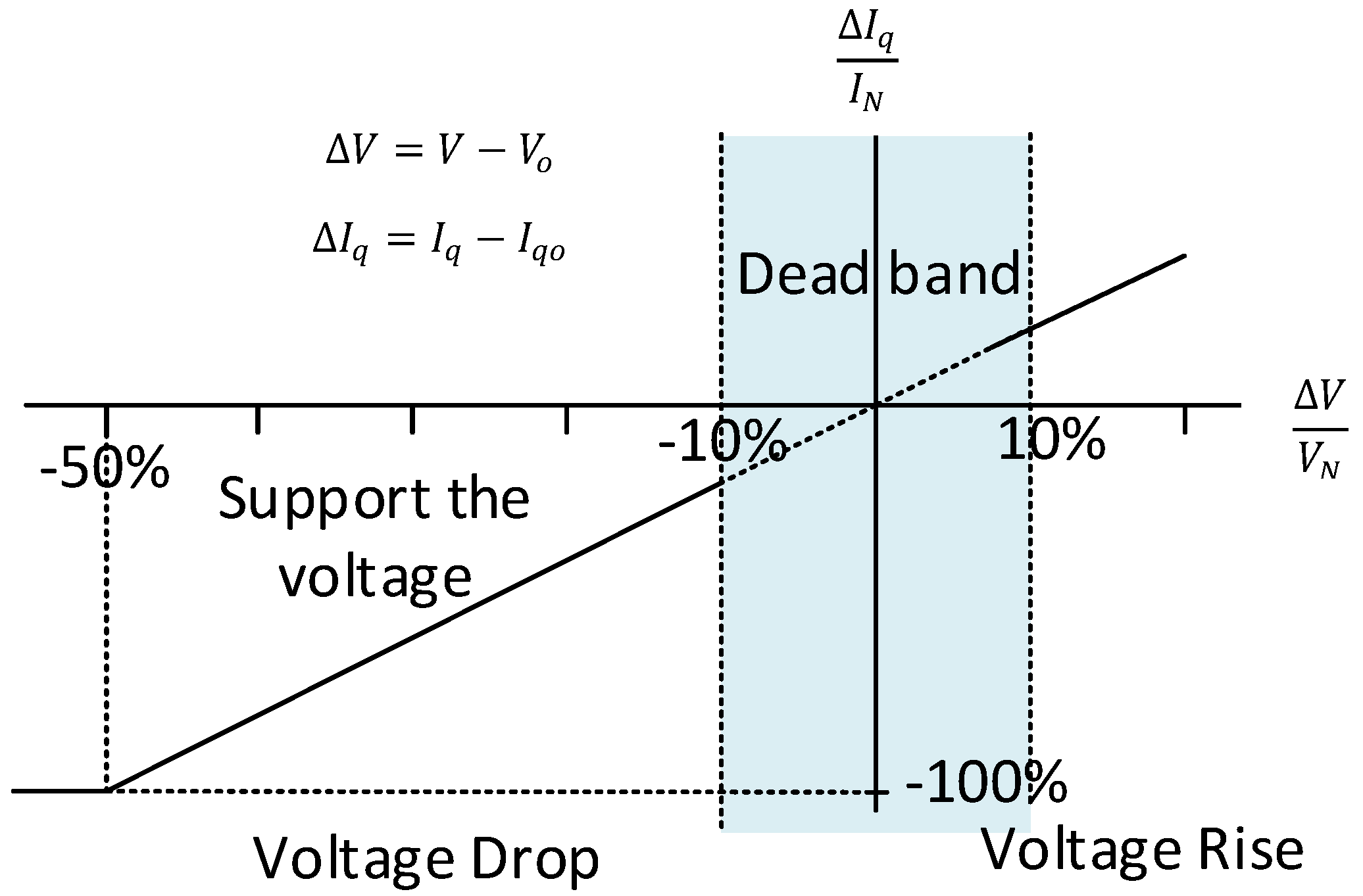
The voltage support requirements as in Figure 2 (usually used in wind-turbines applications) were considered in determining the required level of reactive power injection [15,23]. Voltage support requirements specify the amount of reactive power supplied to the grid for supporting the voltage recovery according to the depth of the voltage sag. For example, from Figure 2, it can be seen that no reactive power injection is required as long as the grid voltage stays in the dead-band region (i.e., $0.9V_N\le V_g\le 1.1V_N$). On the other hand, if the grid voltage drops below 90% of the nominal value, reactive power injection is required according to Equation (1), as given in [8]:

$$\{\begin{array}{ccc}{I}_q=2\left(1-V_g\right)I_N& for& 0.5 p.u\le V_g\le 0.9 p.u\\ I_q=I_N& for& V_g<0.5 p.u\end{array}$$

(1)

where $I_q$ is the reactive current, $I_N$ is the rated current, and $V_g$ is the grid voltage in per unit.

It is worth mentioning that reactive power injection requirements during LVRT differ from one country to another. For example, the reactive current requirements in the Chinese grid [24] specify different compensation levels and has different boundaries when compared to Equation (1) as in German grid requirements. For German grid, a voltage sag at or below 50% requires 100% reactive power compensation (i.e., $I_q=I_N$). In contrast, for the Chinese grid, a voltage sag of 50% requires 60% reactive power compensation (i.e., $I_q=0.6I_N$) and for a voltage sag of 80% and below the reactive power requirement is at 105% (i.e., $I_q=1.05I_N$).

A FLC controller is configured to estimate the PF at which the active and reactive power are injected into the grid. The FLC has two inputs; one is the magnitude of the voltage at the PCC, and the second input is the power level available from the PV system. The FLC is implemented with the objective to enhance the reactive power injection by minimizing the inverter’s maximum current limitation. For an inverter to support the LVRT operation, as explained above, the minimum value of its predesigned current rating $\left(I_{max}\right)$ should be at least at $2.25I_N$ in the constant average active power strategy [8]. However, in a PV system, the amount of active power delivered by the inverter depends on the level of the solar irradiation, and thus the full capacity of the inverter may not be utilized at all times; hence, the utilization factor of the inverter becomes very low.

The proposed FLC examines how severe the voltage sag is, and the level of real power available from the PV system to decide the level of reactive power injection and the de-rating of the inverter power by adjusting the inverters PF angle. For example, if the voltage sag is small and PV power is high, then PF angle is small. On the other hand, for the small voltage sag and low PV power, the PF angle will be large (i.e., all the inverter capacity will be dedicated to the reactive power injection).

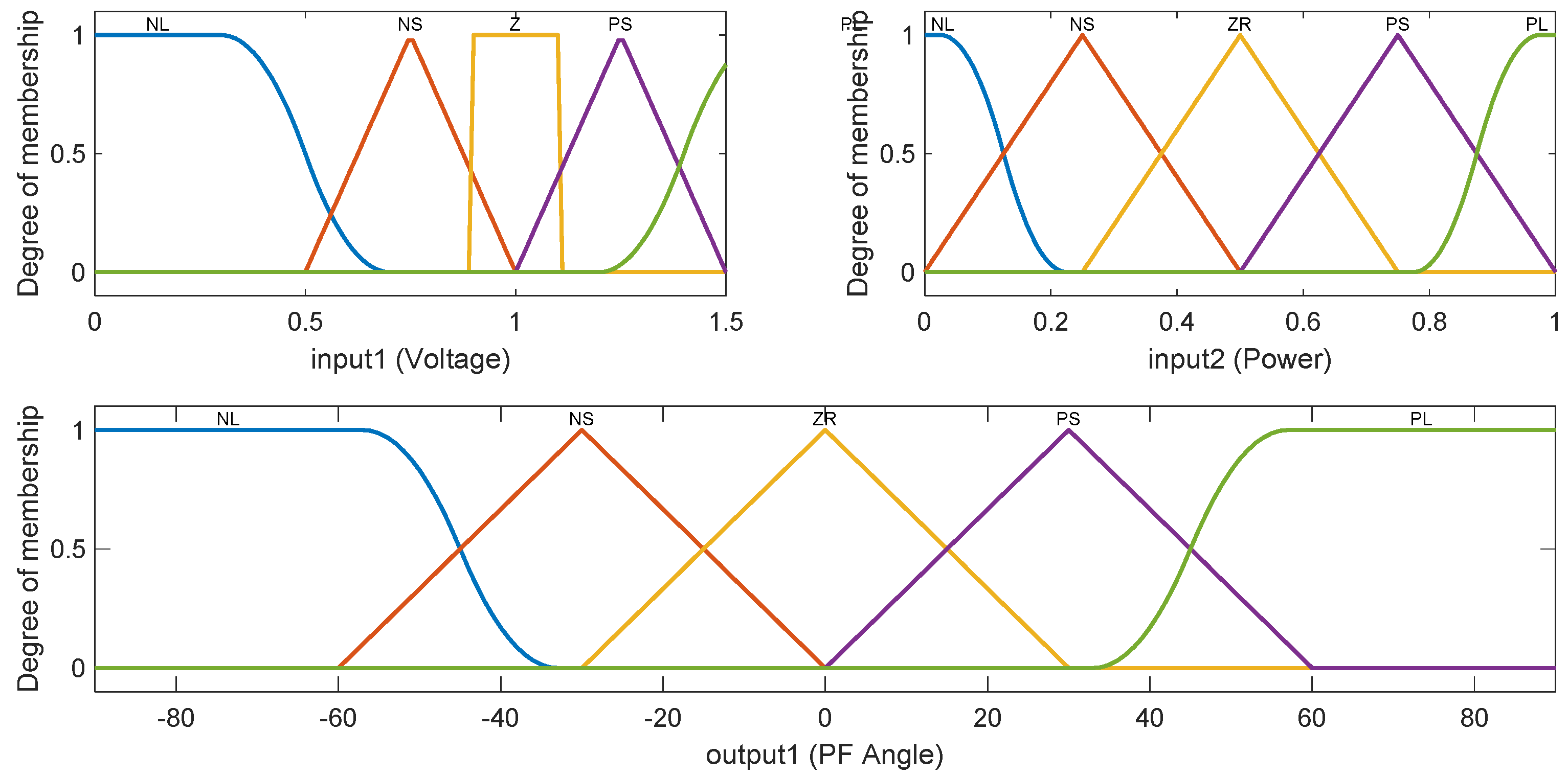
The implemented FLC is characterized by having five membership functions for each input, 25 rules with Mamdani fuzzy inferencing system (FIS), and a defuzzification method that uses the Largest of Maximum method (LOM). The voltage support requirements, and level of available power from the PV influenced the design of the inputs and output membership functions, as depicted in Figure 3 and fuzzy rules as in

Table 1. Fuzzy rules.

	Input 2 (P)	NL No Power	NS Low	ZR Medium	PS High	PL Full
Input 1 (V)
NL (very low)		PL (max leading PF)	PL (max leading PF)	PL (max leading PF)	PL (max leading PF)	PL (max leading PF)
NS (low)		PL (max leading PF)	PS (medium leading PF)	PS (medium leading PF)	PS (medium leading PF)	PS (medium leading PF)
ZR (nominal)		ZR (unity PF)	ZR (unity PF)	ZR (unity PF)	ZR (unity PF)	ZR (unity PF)
PS (high)		ZR (unity PF)	ZR (unity PF)	NS (medium lagging PF)	NS (medium lagging PF)	NS (medium lagging PF)
PL (very high)		NL (max lagging PF)	NL (max lagging PF)	NL (max lagging PF)	NL (max lagging PF)	NL (max lagging PF)

Input 1: Voltage at PCC, Input 2: PV power level, Output 1: PF angle. Negative Large (NL), Negative Small (NS), Zero (ZR), Positive Small (PS), Positive Large (PL).

. Although it is not addressed in this paper, in Figure 3, the range of the voltage input membership extends above 1.1, which represents the operation when the inverter is required to absorb reactive power in case the grid voltage experiences an over voltage.

In addition to the FLC, a PQ calculator is implemented in this work to perform two main functions: it firstly monitors the commanded power to the inverter and ensures that it does not exceed the rated capacity of the inverter without de-rating the real power and using the FLC recommended reactive power injection. If the output exceeds the rated KVA capacity of the inverter, the PQ calculator will de-rate the output real power according to Equation (2):

$$P_{in}^{*}=\sqrt{S_r^2-Q_{in}^{*}}$$

(2)

where, $S_r$ is the rated KVA of the inverter, $P_{in}^{*} \mathrm{and} Q_{in}^{*}$ are the inverter commanded active and reactive power, respectively.

The second function of the PQ calculator is to reset the reference real power of the inverter to zero whenever the voltage sag drops below 50% of its nominal value.

2.3. Power Angle (δ) Regulator

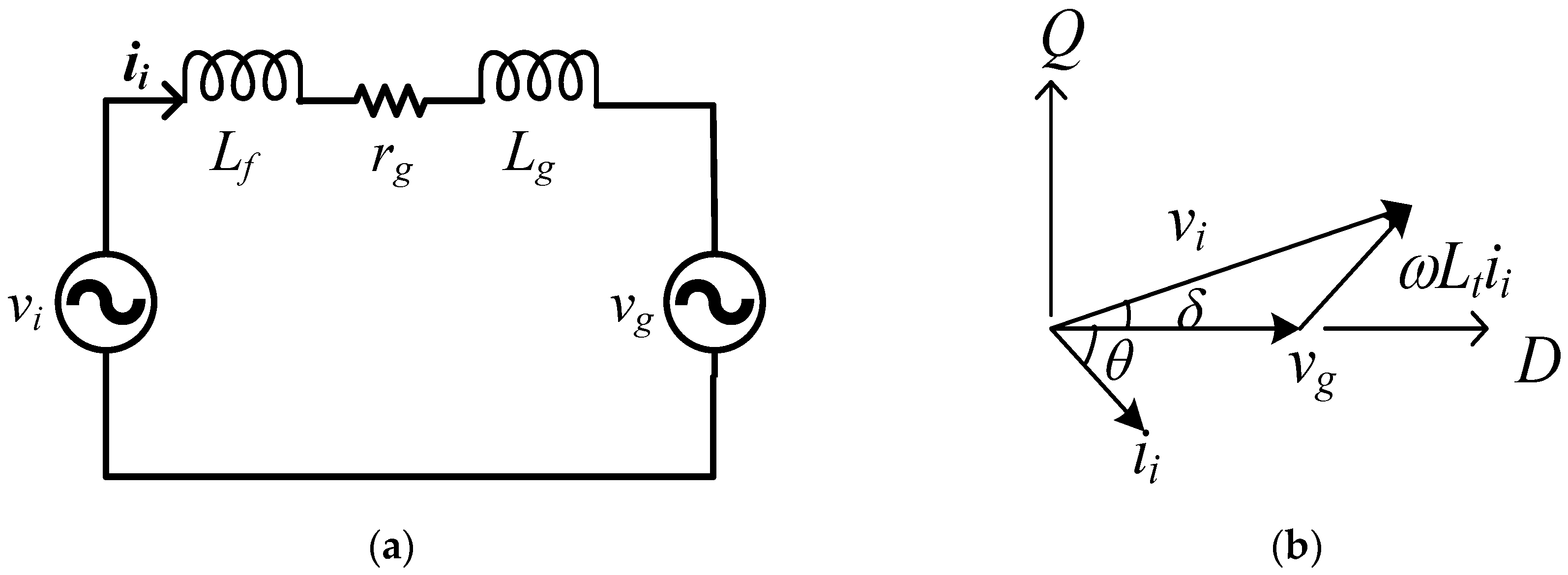
With reference to Figure 4, the active power supplied to the grid in steady state (with inductor resistances ignored) can be given as:

$$P=\frac{V_i{V}_g}{2X_t}\sin \left(\delta \right)\approx \frac{V_i{V}_g}{2X_t}\delta$$

(3)

where $V_i \mathrm{and} V_g$ are, respectively, the peak voltage of inverter and grid, $X_t$ is the reactance of the line inductance, $\delta$ is the power angle and for small $\delta$, $\sin \left(\delta \right)\approx \delta$.

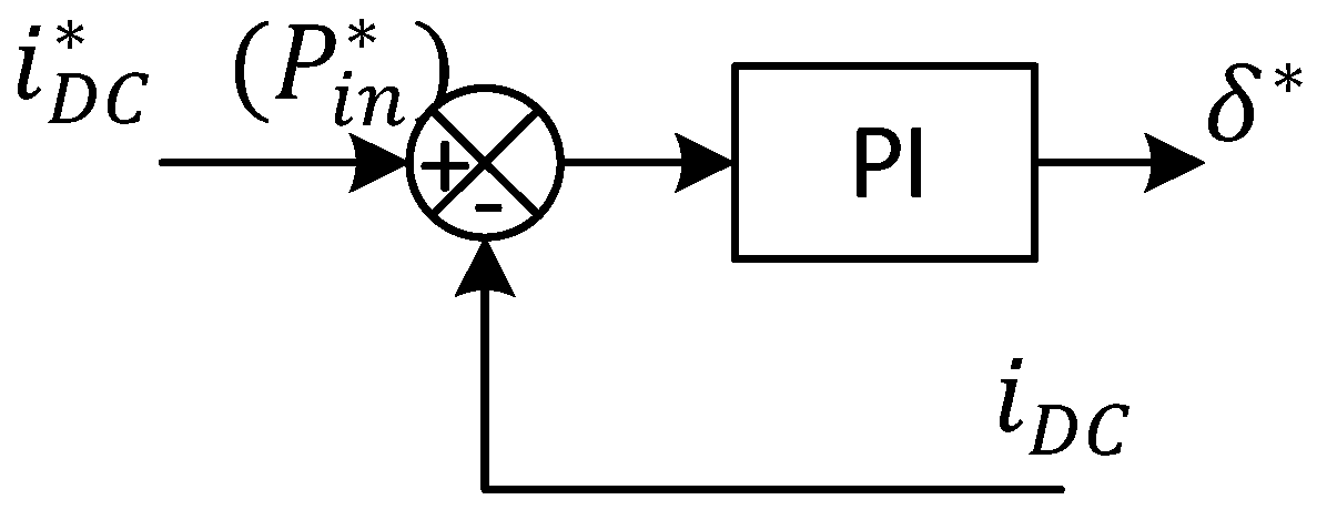
A PI regulator is implemented as in Figure 5 to control the power angle of the inverter and hence the real power to be injected into the grid. The PI controller operates on the error between the reference power ($P_{in}^{*}$) obtained from the PQ calculator, and inverter DC-link current ($i_{DC}$). The DC-link current, is measured, filtered, and regulated to track the reference power command by controlling the power angle ($\delta$) of the PWM command signal. The regulation scheme is shown in Figure 5.

In this regulation scheme, it is assumed that the inverter is lossless [15,25]; thus, the instantaneous power balance at both sides of the inverter can be expressed as in Equation (4):

$$p_{DC}\left(t\right)=p_{AC}\left(t\right)$$

(4)

using the space vector representation of the circuit in Figure 4, Equation (4) can be written as [8]:

$$v_{DC}\left(t\right)i_{DC}\left(t\right)=\frac{v_{iD}\left(t\right)i_{iD}\left(t\right)+v_{iQ}\left(t\right)i_{iQ}\left(t\right)}{2}$$

(5)

where, $v_{iD}, v_{iQ}$ and $i_{iD}, i_{iQ}$ are the D and Q components of the inverter space vector output voltage and current, respectively.

The state space equations of the inverter voltages and currents in the DQ reference frame can be expressed as:

$$v_i\left(t\right)=v_g\left(t\right)+r_g{i}_i\left(t\right)+\left(\rho +j\omega \right)L_t{i}_i\left(t\right)$$

(6)

where $\rho =d/dt$ (is the differential operator). The DQ components can then be obtained as:

$$v_{iD}\left(t\right)=v_{gD}\left(t\right)+\left(\rho L_t+r_g\right)i_{iD}\left(t\right)-\omega L_t{i}_{iQ}\left(t\right)$$

(7)

and,

$$v_{iQ}\left(t\right)=v_{gQ}\left(t\right)+\left(\rho L_t+r_g\right)i_{iQ}\left(t\right)+\omega L_t{i}_{iD}\left(t\right)$$

(8)

In Equations (7) and (8), if the grid is assumed constant (voltage and frequency), and the inverter voltage is sinusoidal, then the grid and inverter voltages become:

$$v_{gQ}\left(t\right)=0$$

and,

$$v_{gD}\left(t\right)=v_g\left(t\right)=V_g$$

(9)

and for the inverter,

$$v_{iD}\left(t\right)=V_i\cos \left(\delta \left(t\right)\right)$$

and,

$$v_{iQ}\left(t\right)=V_i\sin \left(\delta \left(t\right)\right)$$

(10)

Equations (9) and (10) can be linearized around an operating point and used together with Equations (5), (7), and (8) to find a reduced linear model of the inverter-grid system. This linear model relates the change of the power angle and the DC-link current. Linearizing around ${\delta }_o$:

$$\delta \left(t\right)={\delta }_o+\Delta \delta \left(t\right)$$

(11)

$$\Delta v_{iD}\left(t\right)=(-V_{io}\sin {\delta }_o)\Delta \delta \left(t\right)$$

(12)

similarly, the quadrature component can be written as,

$$\Delta v_{iQ}\left(t\right)=(V_{io}\cos {\delta }_o)\Delta \delta \left(t\right)$$

(13)

Also, Equations (7) and (8) can be written in linear form as:

$$\Delta v_{iD}\left(t\right)=\left(\rho L_t+r_g\right)\Delta i_{iD}\left(t\right)-\omega L_t\Delta i_{iQ}\left(t\right)$$

(14)

and,

$$\Delta v_{iQ}\left(t\right)=\left(\rho L_t+r_g\right)\Delta i_{iQ}\left(t\right)+\omega L_t\Delta i_{iD}\left(t\right)$$

(15)

If $V_{DC}\left(t\right)$ is assumed constant, then from Equation (4), the change in the DC-link current around the operating point for a change in the power angle can be written as:

$$\Delta i_{DC}\left(t\right)=\frac{\Delta v_{iD}\left(t\right)i_{iDo}+v_{iDo}\Delta i_{iD}\left(t\right)+\Delta v_{iQ}\left(t\right)i_{iQo}+v_{iQo}\Delta i_{iQ}\left(t\right)}{2V_{DC}}$$

(16)

Therefore, the response of the DC-link current to change in the power angle can be obtained by Equation (16); and the transfer function can be written as:

$$\frac{I_{DC}\left(s\right)}{\delta \left(s\right)}=\frac{K}{{(s+\frac{r_g}{L_t})}^2+{\omega }^2}$$

(17)

where $K=\frac{\omega V_{io}^2}{2V_{DC}{L}_t}$ and it depends on the inverter parameters.

2.4. Reactive Power Regulation

The reactive power flow between the inverter and the grid is controlled by regulating the inverter’s output voltage at the PCC. Similar to the discussion in Section 2.3, if the inverter’s power angle is small, the reactive power into the grid system can be given as:

$$Q=\frac{V_g\left(V_{i}cos\delta -V_g\right)}{2X_t}\approx \frac{V_g}{2X_t}\left(V_i-V_g\right)$$

(18)

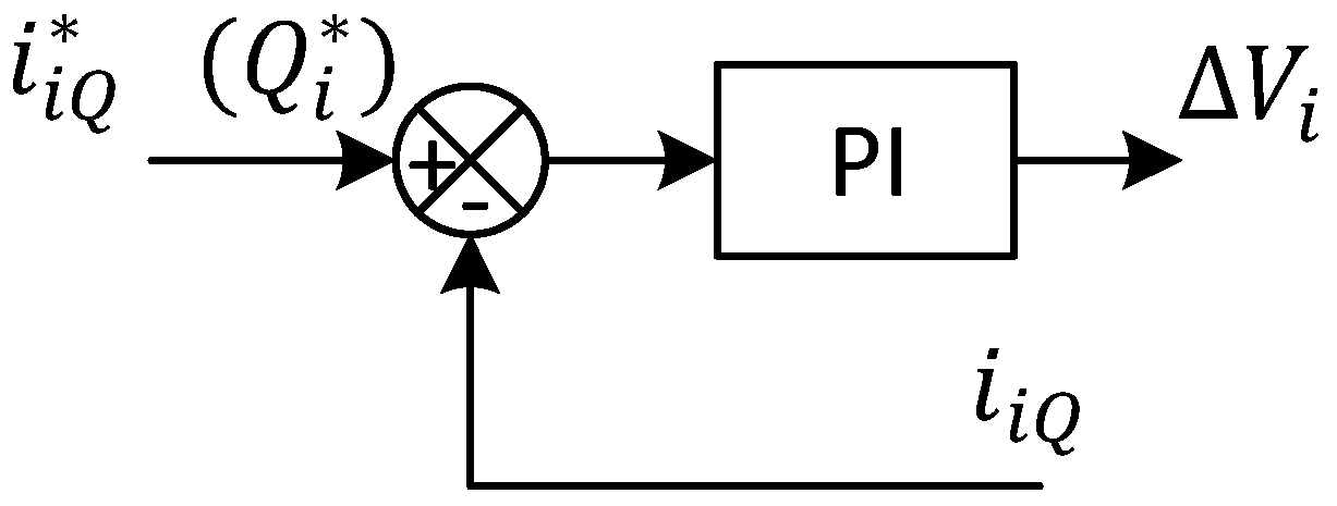
From Equation (18), it can be seen that in steady state, the reactive power flow is related to the difference between the inverter and the grid voltages. The reactive power regulation scheme is carried out by controlling the quadrature component of the inverter current ($i_{iQ}$). The current $i_{iQ}$ is regulated to track a reference value that is calculated based on the grid reactive power demand ($Q_i^{*}$). The PI controller in Figure 6 will continuously regulate the inverter’s output voltage by adjusting the voltage modulation index based on the reactive power command.

Following the same procedure as in Section 2.3, and linearizing and simplifying the equations, the response of the inverter’s reactive power to change in the inverter’s output voltage can be written as:

$$\frac{\Delta Q_i\left(s\right)}{\Delta V_i\left(s\right)}=\frac{K_1}{{(s+\frac{r_g}{L_t})}^2+{\omega }^2}$$

(19)

where $K_1=\frac{\omega V_{io}}{L_t}$ and it depends on the inverter parameters.

The proportional and integral gains of the PI controllers were obtained by using the PI tuner facility in Simulink. However, to optimize the actual system response, the gains were fine-tuned and readjusted manually around the Simulink values.

3. Simulation Results and Discussion

To examine the effectiveness of the proposed system, a simulation study was carried out using Simulink from MATLAB. The simulation cases were grouped to represent two conditions: Case (1), the day mode, and Case (2), the cloudy and night mode. The parameters and specifications of the system under investigation are given in

Table 2. System specifications.

Inverter Rated Power (Srated)	2 kVA	PWM Switching Frequency (fs)	10 kHz
Filter Inductance (Lf)	25 mH	Grid Voltage Vg(rms)	230 V
Grid Side Inductance (Lg)	0.5 mH	Grid Frequency (fg)	50 Hz
Grid Side Resistance (rg)	0.64 Ω	Inverter Input DC Voltage (VDC)	400 V
Filter Capacitor (Cf)	1.5 µF	Power Angle PI Regulator Kp, Ki	2 × 10−3, 1.58
DC Link Capacitor (Cdc)	1000 µF	Reactive Power PI Regulator Kp, Ki	0.01, 10

.

3.1. Case I: Daytime Operation

The daytime operation corresponds to the situation when the PV system is supplying maximum real power to the grid, i.e., the inverter full capacity is utilized to supply real power. Under this scenario, the grid voltage is stepped down to 75%, 50%, and 10%.

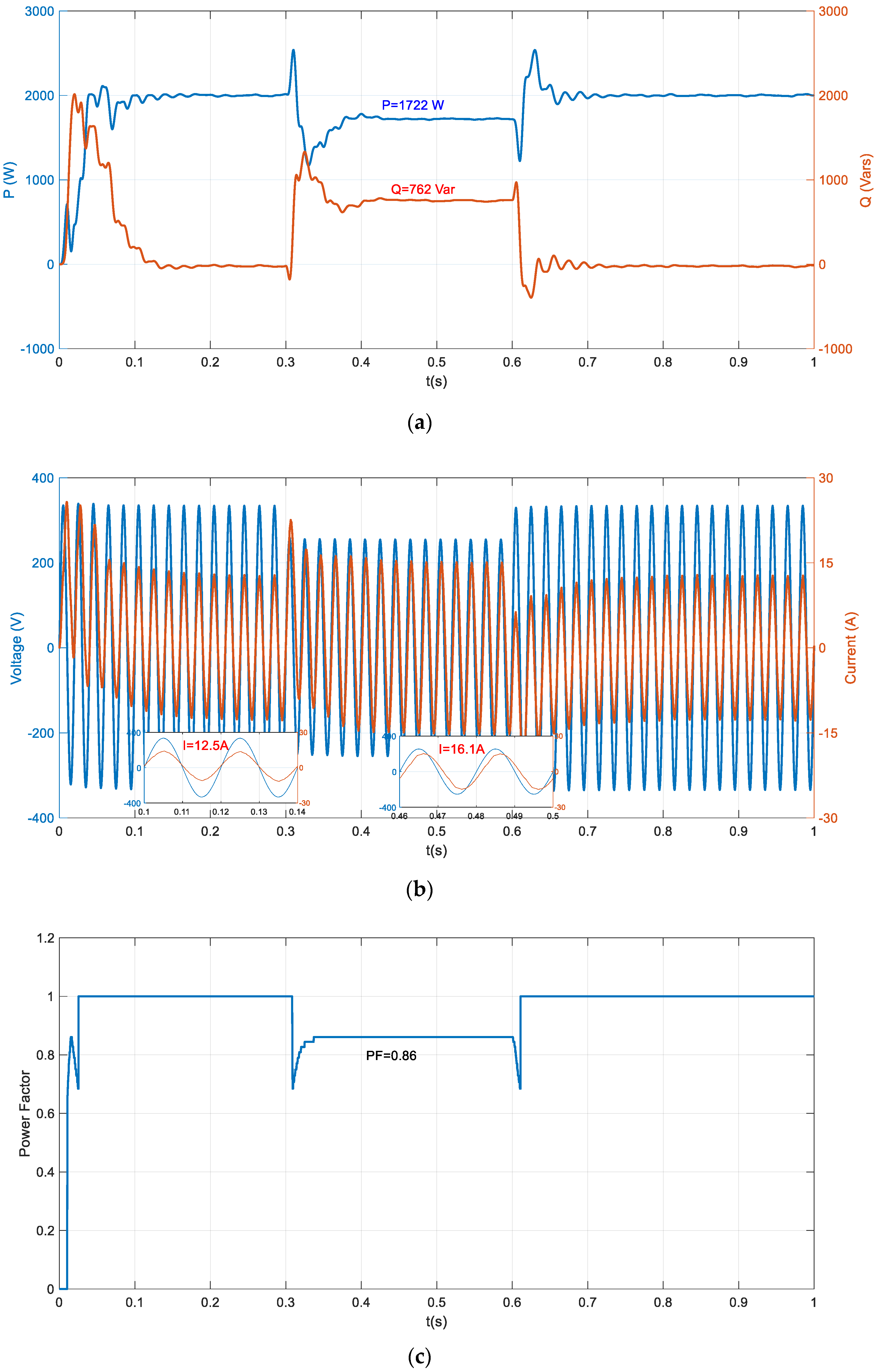
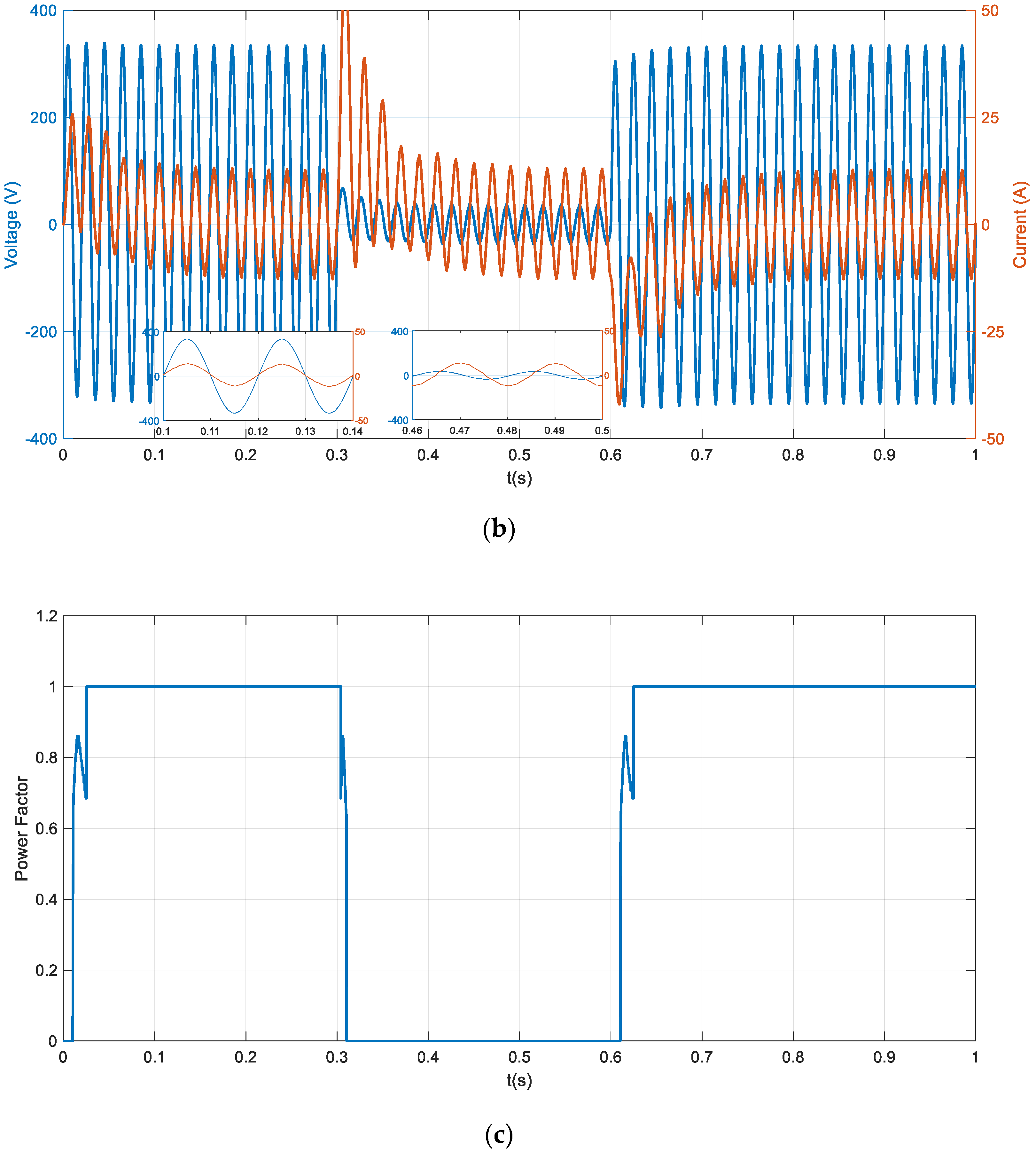
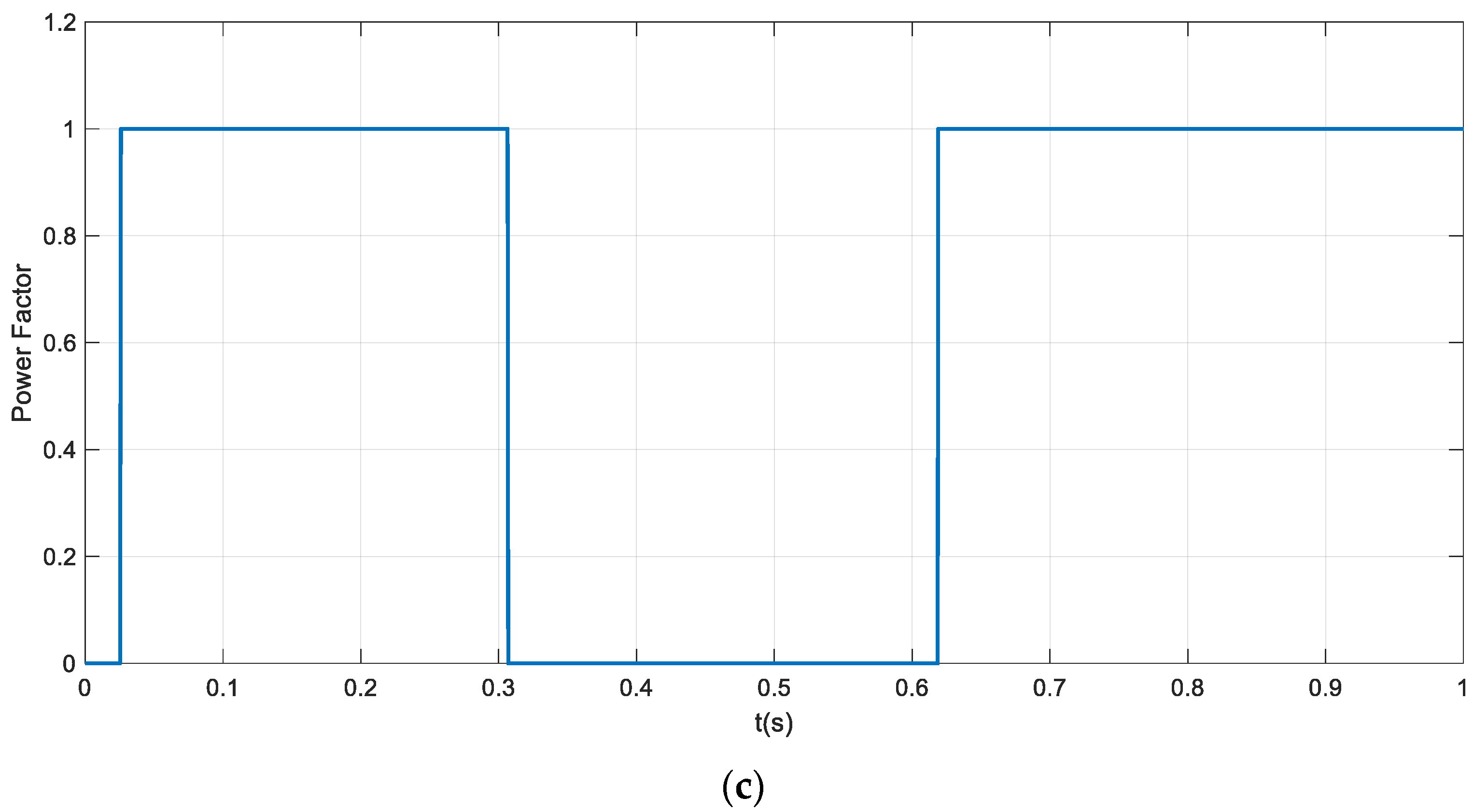
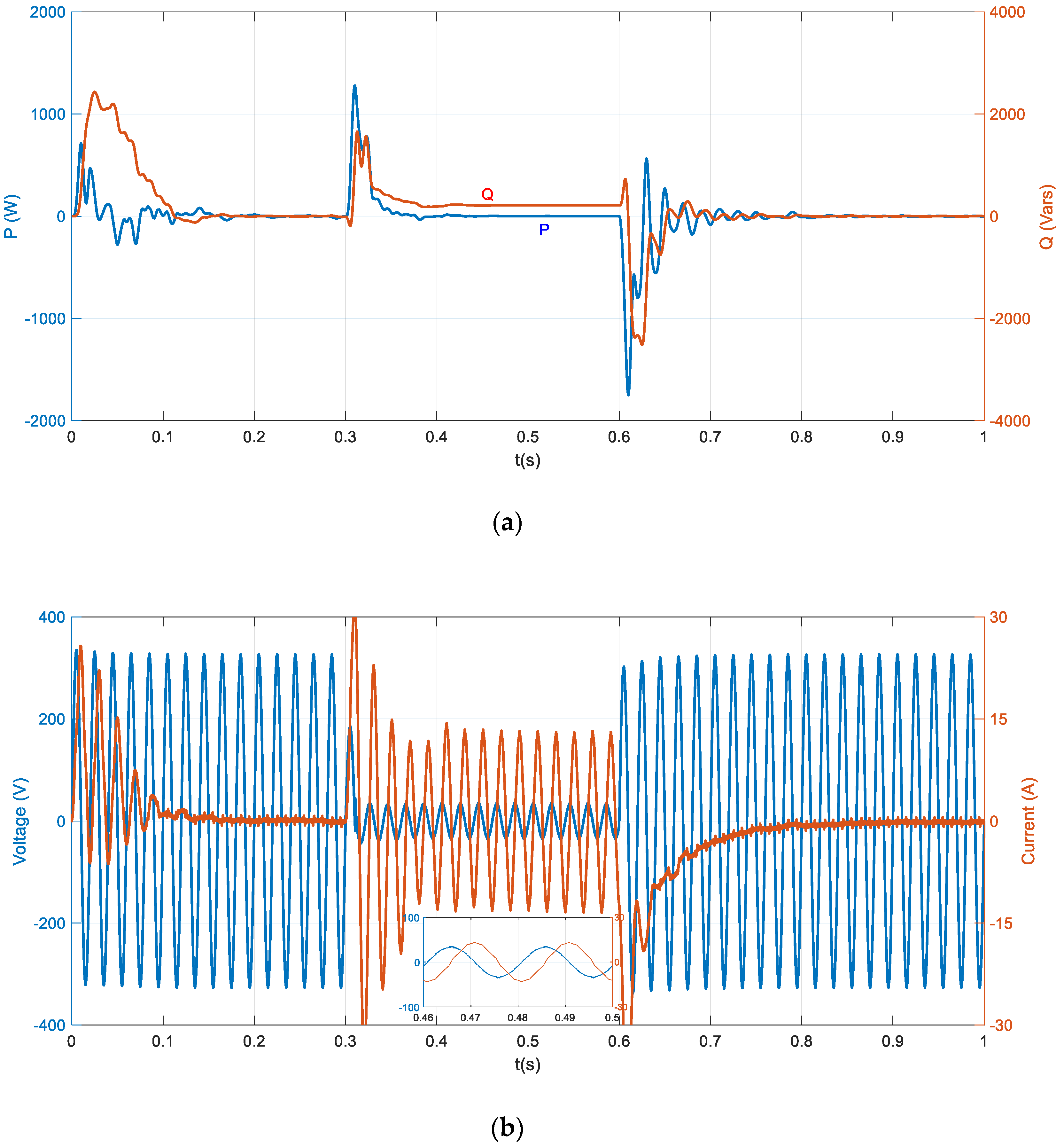
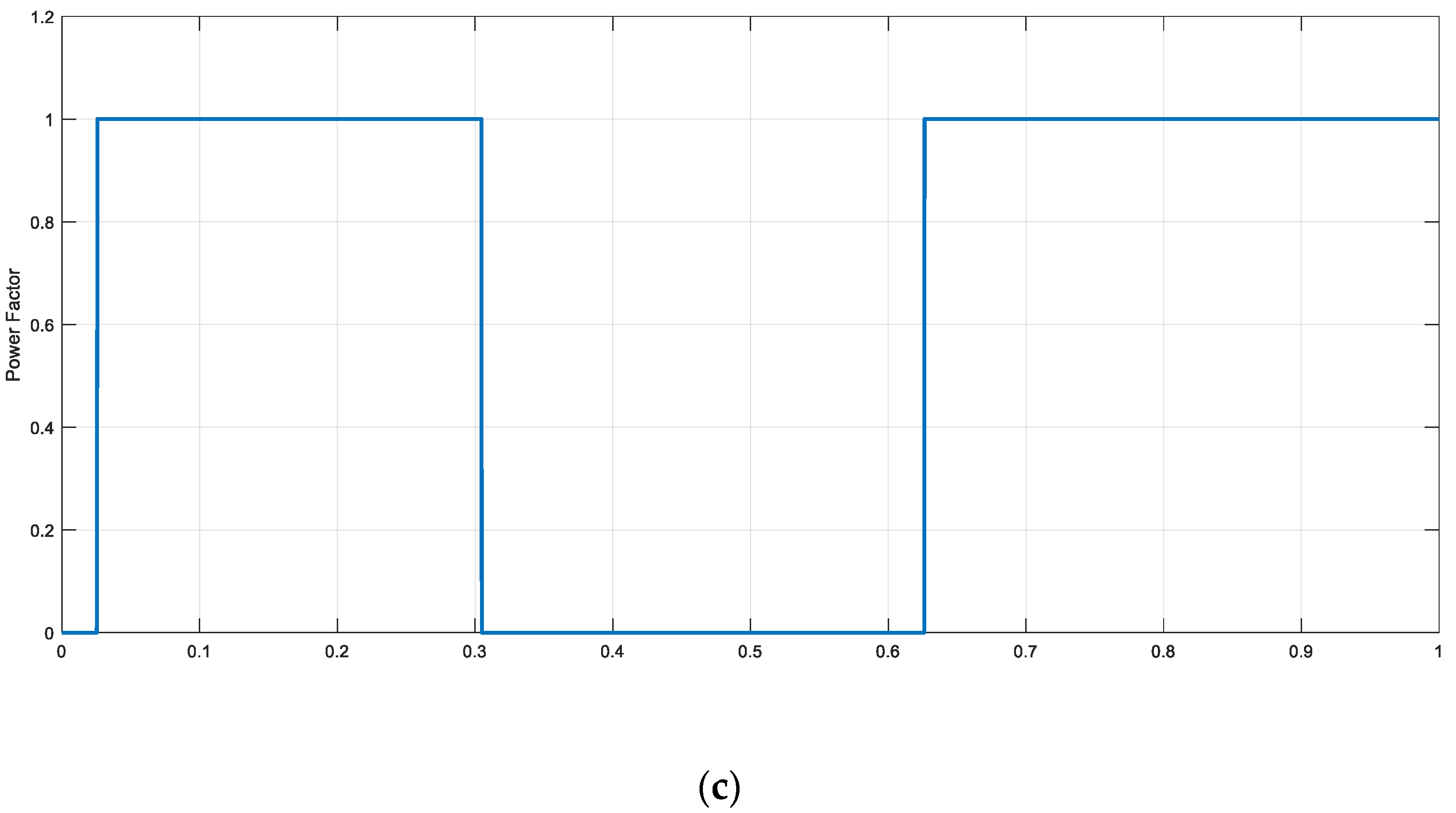
The simulation results in Figure 7a–c show the output power (P, and Q), voltage and current (V, and I), and power factor, respectively. At time t = 0.3 s, the grid voltage dropped to 75% of the nominal value and the drop lasted until t = 0.6 s. The simulation results show that the active power injected into the grid was de-rated below the operating value to allow injection of reactive power, and hence supporting the grid voltage. From Figure 7c, PF is calculated by the FLC at 0.86, and hence the de-rated power is obtained as 1722 (= 2000 × 0.86) W, and the reactive power at the 230 V level is 1016 (= 762/0.75) Vars. Figure 7b shows the voltage and current signals during and outside the voltage sag region. It can be observed that the current leads the voltage during the voltage sag, and is in phase with it during normal operation. This indicates reactive power flow from the inverter during the sag and unity PF operation outside the sag region.

It was also observed that during the voltage sag, the inverter current increased to 16.1 A (peak). The increase in current is logical since the inverter has to supply this current at the PCC, which is 75% of the nominal value. This value of the current is about $1.3\times I_{rated}$ which is well below the $2.25\times I_{rated}$ criteria quoted earlier for constant average active power scheme.

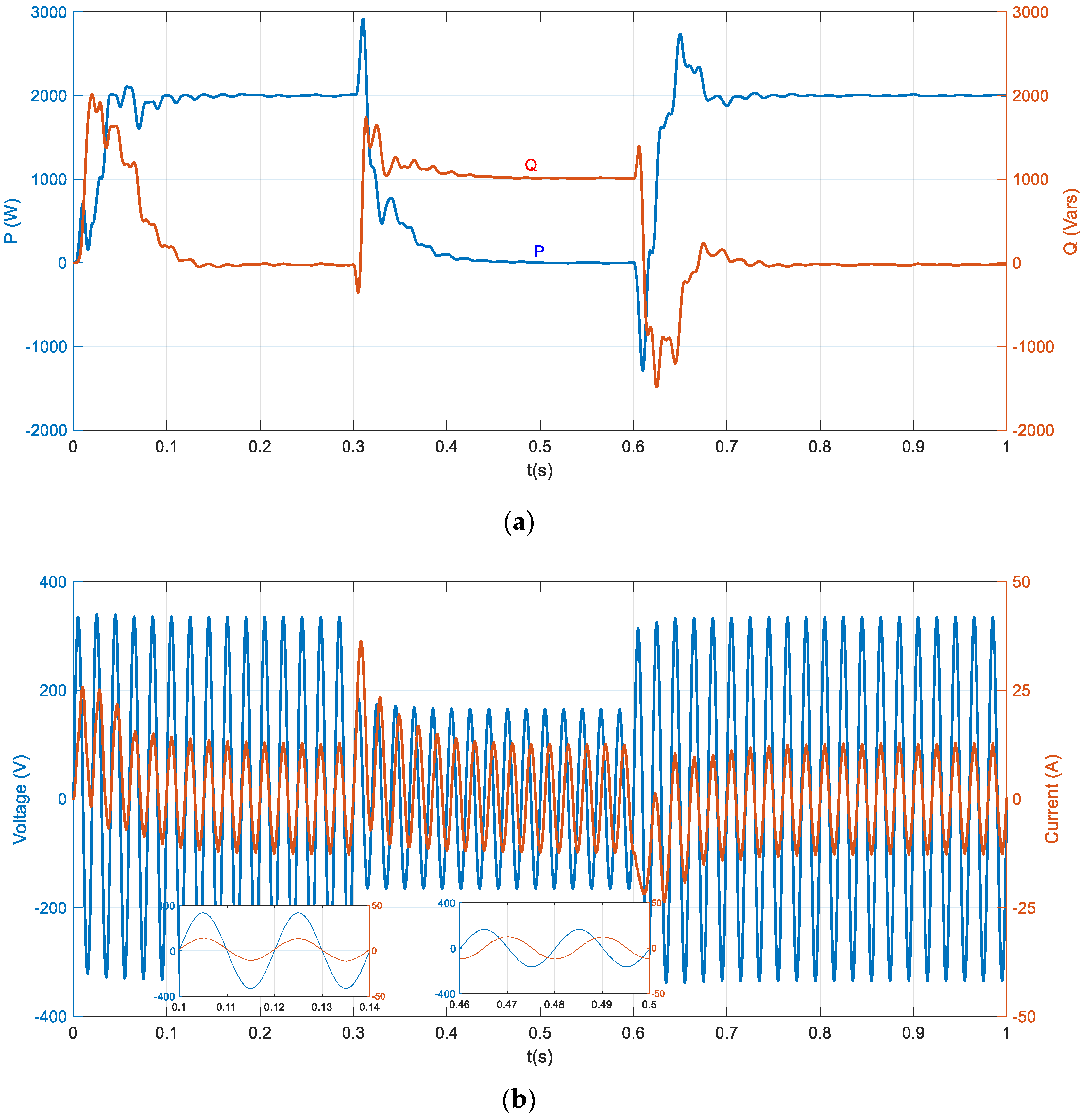
Figure 8a–c show the simulation results when the system is running under the same operating conditions, as in Figure 7, but this time, the voltage level was set to 50%. The simulation results show that the active power injected into the grid has been de-rated to zero value, allowing maximum injection of reactive power, and thus providing support to the grid voltage. The FLC reduced the PF from unity to zero (i.e., the current leads the voltage by 90°) as in Figure 8c. In this simulation case, it can be seen that the full capacity of the inverter was utilized to supply reactive power to the grid during the voltage sag. Again, from Figure 8a, the reactive power is at approximately 1000 Vars, which is supplied at 50% voltage sag, thus, at nominal voltage level, this corresponds to (1000/0.5 =) 2000 Vars. The current and voltage signals in Figure 8b are 90° out of phase during the voltage sag, and are in phase during the normal mode of operation.

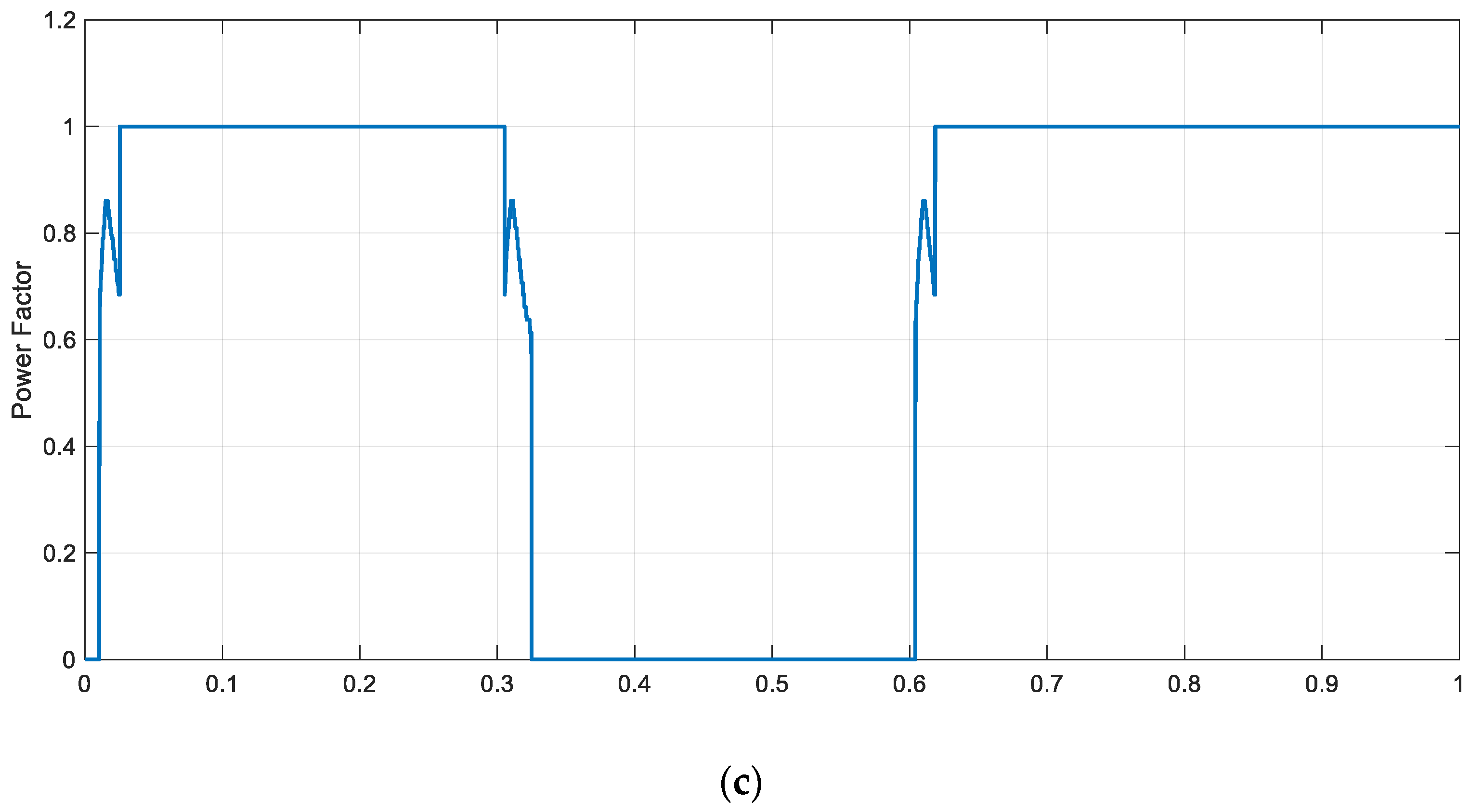
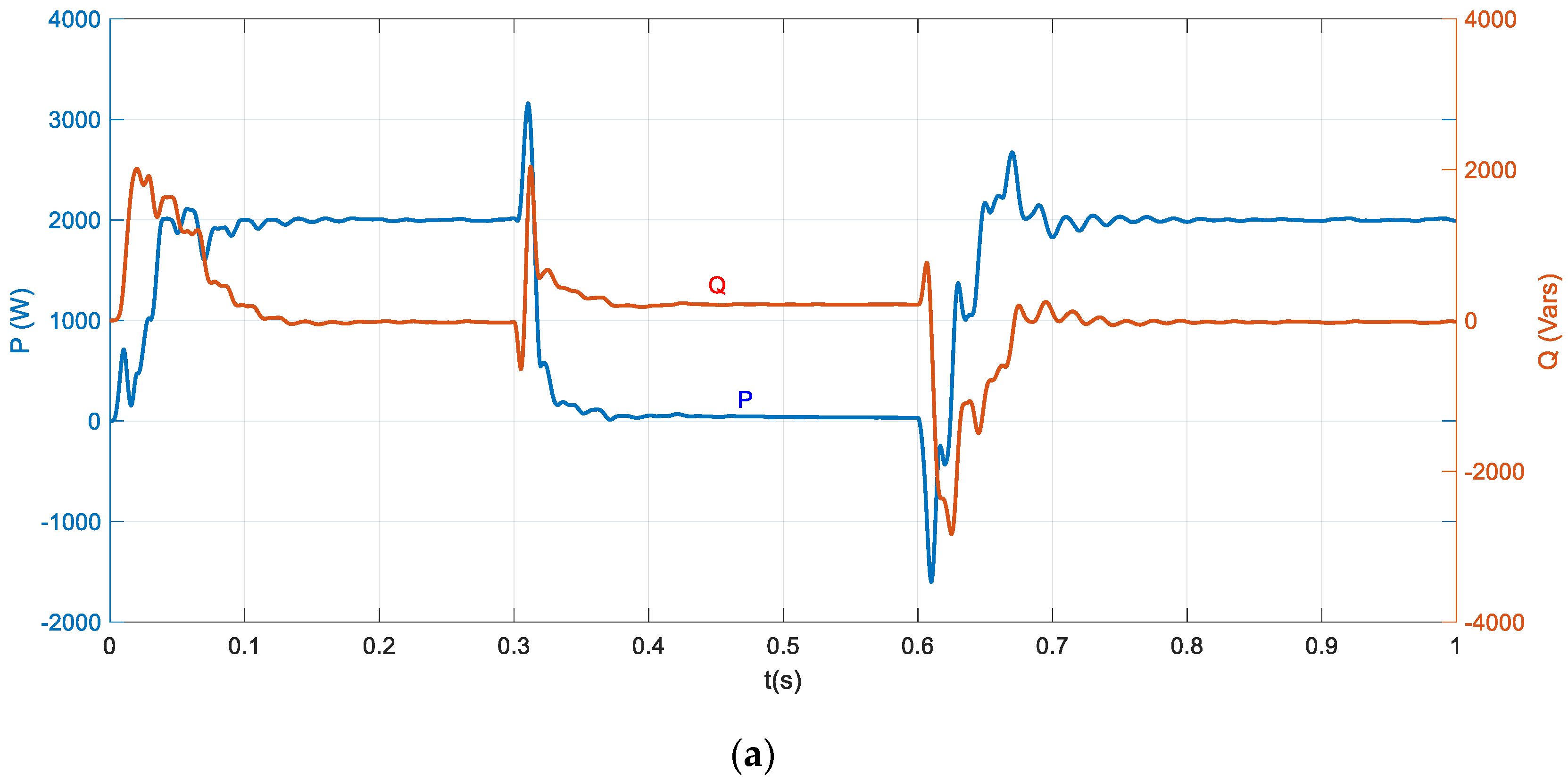
In Figure 9, the system is examined during a severe voltage sag condition at 10% of the nominal voltage. The active power was de-rated to zero and full reactive power injection was achieved as shown in Figure 9a. This is evident, as well, from the current signal in Figure 9b. The current is at a rated level and leads the voltage by 90°. The results conform with the results in [25] for zero-voltage ride-through, and with the statement quoted in [8]: “When severe voltage fault happens, the PV system should inject full reactive power without delivering active power to the grid”. Figure 9c shows the PF has been reduced to zero during the voltage sag.

3.2. Case II: Cloudy and Nighttime Operation

In this mode of operation, two scenarios are addressed: the first, when the input power from the PV system is at 40%, to resemble a cloudy day operation; and the second when PV power is at 0% representing (nighttime).

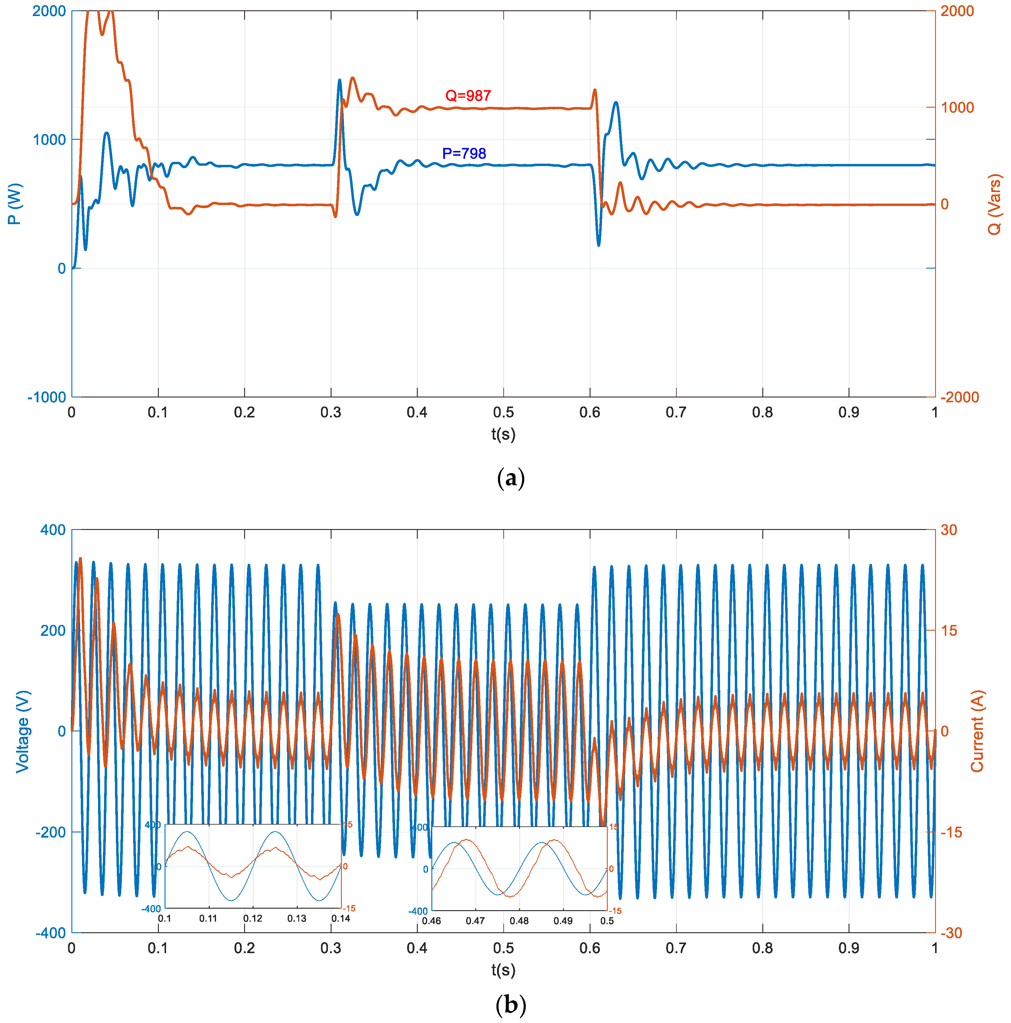
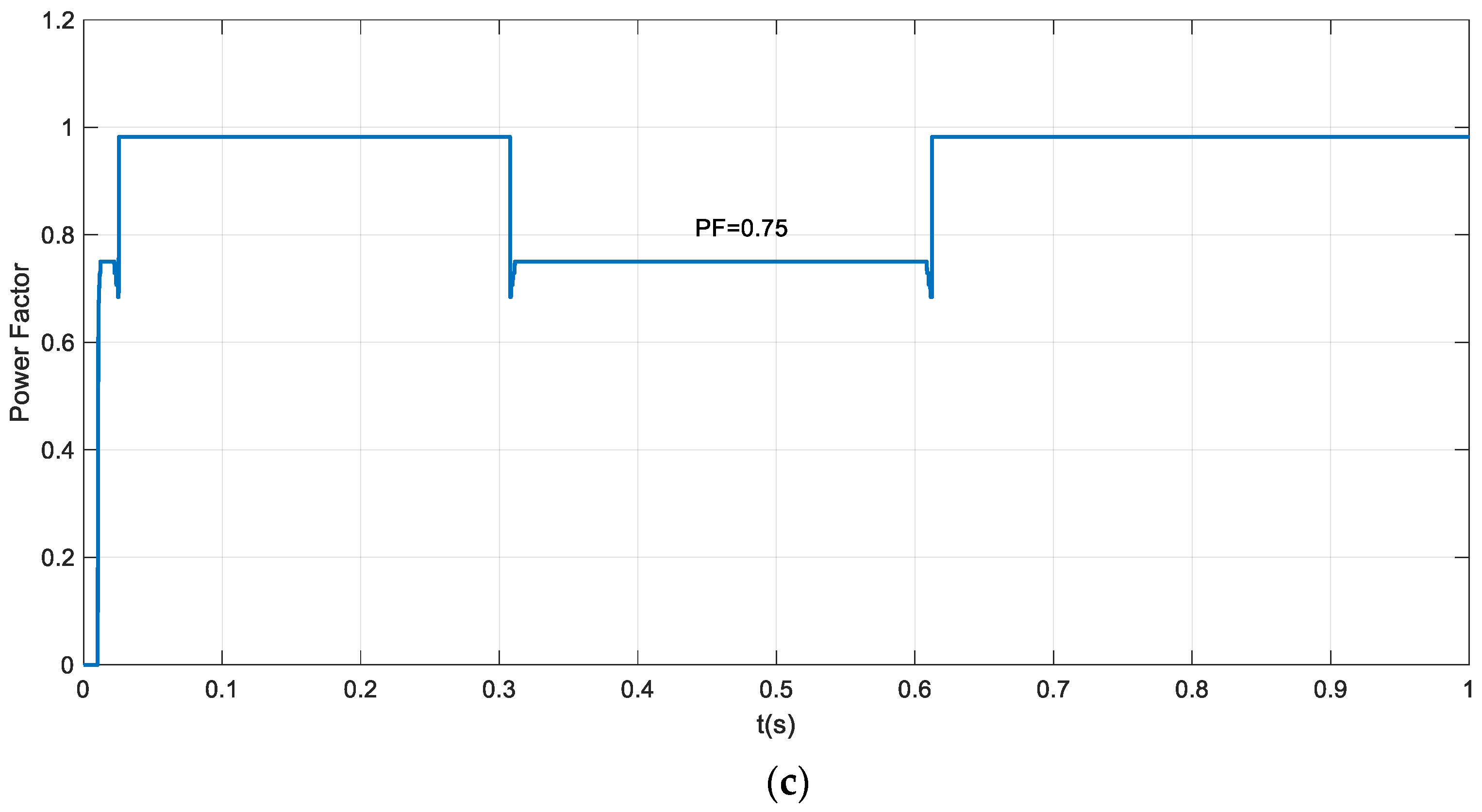
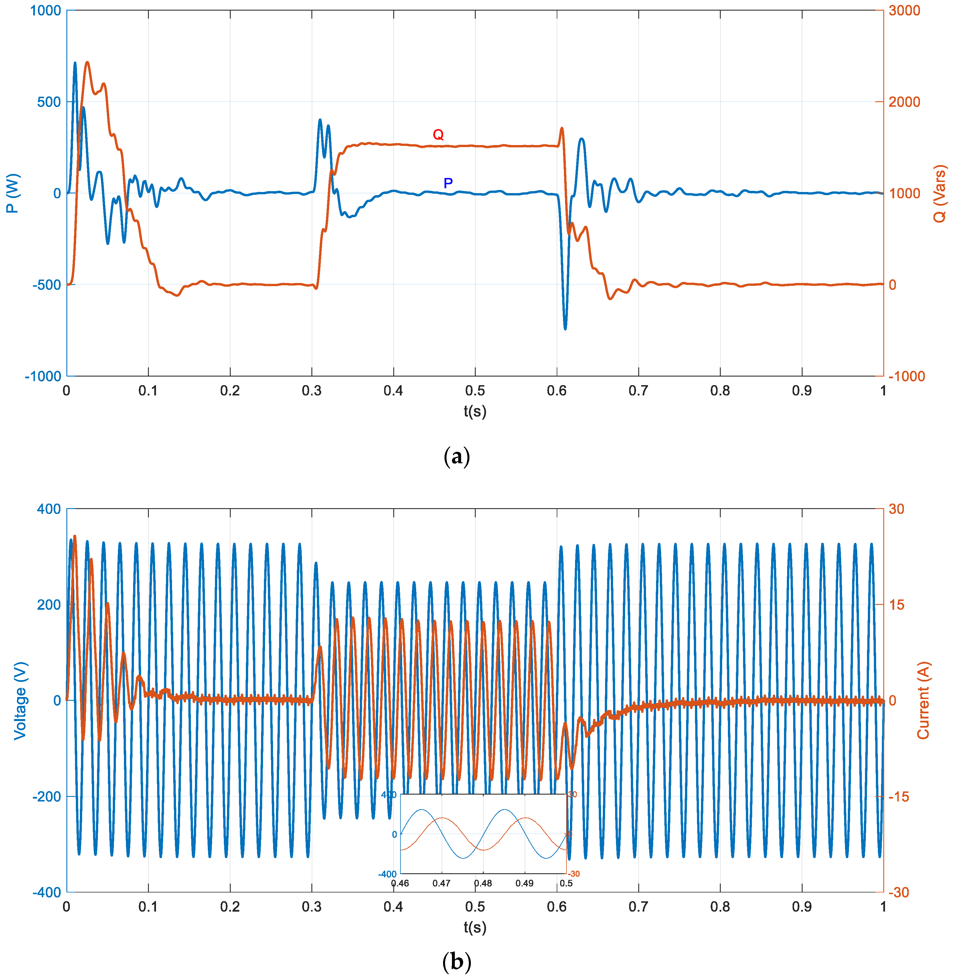
For the cloudy day operation, only the case of the 25% voltage sag (75% rated voltage) is shown in Figure 10. The obtained results in Figure 10a show that the active power remained constant at approximately 800 W (during and outside the voltage sag region). This means no de-rating of the power occurred since the inverter has only 40% of its capacity being utilized. Therefore, the FLC sets the PF at 0.75, slightly lower when compared to the daytime case (PF = 0.86), which allows for more of the inverter capacity to be used for reactive power compensation. In addition, the reactive power remained at approximately 1000 Vars during the 0.75 p.u. voltage level, which corresponds to $2000\times \sin \left({41.4}^o\right)$ Vars.

Figure 10b,c show, respectively, the voltage and current, and the PF as estimated by the FLC. Again, it was observed that the current outside the sag region stayed close to 5.5 A (peak) and in phase with the voltage corresponding to 800 W. During the voltage sag, the current increased to 10.5 A (peak). This current is made up of an active component of 6.5 A (peak), which corresponds to 800W, and a reactive current of 8.2 A (peak) that corresponds to 1000 Vars, both being delivered to the grid at V_g = 0.75 × V_rated. Note again, that the FLC calculated PF was used to set the reactive power without affecting (de-rating) the real power; hence, the actual power factor of the inverter is $\cos \left(ta{n}^{-1}\left(\frac{8.2}{6.5}\right)\right)=0.62 \mathrm{leading}.$

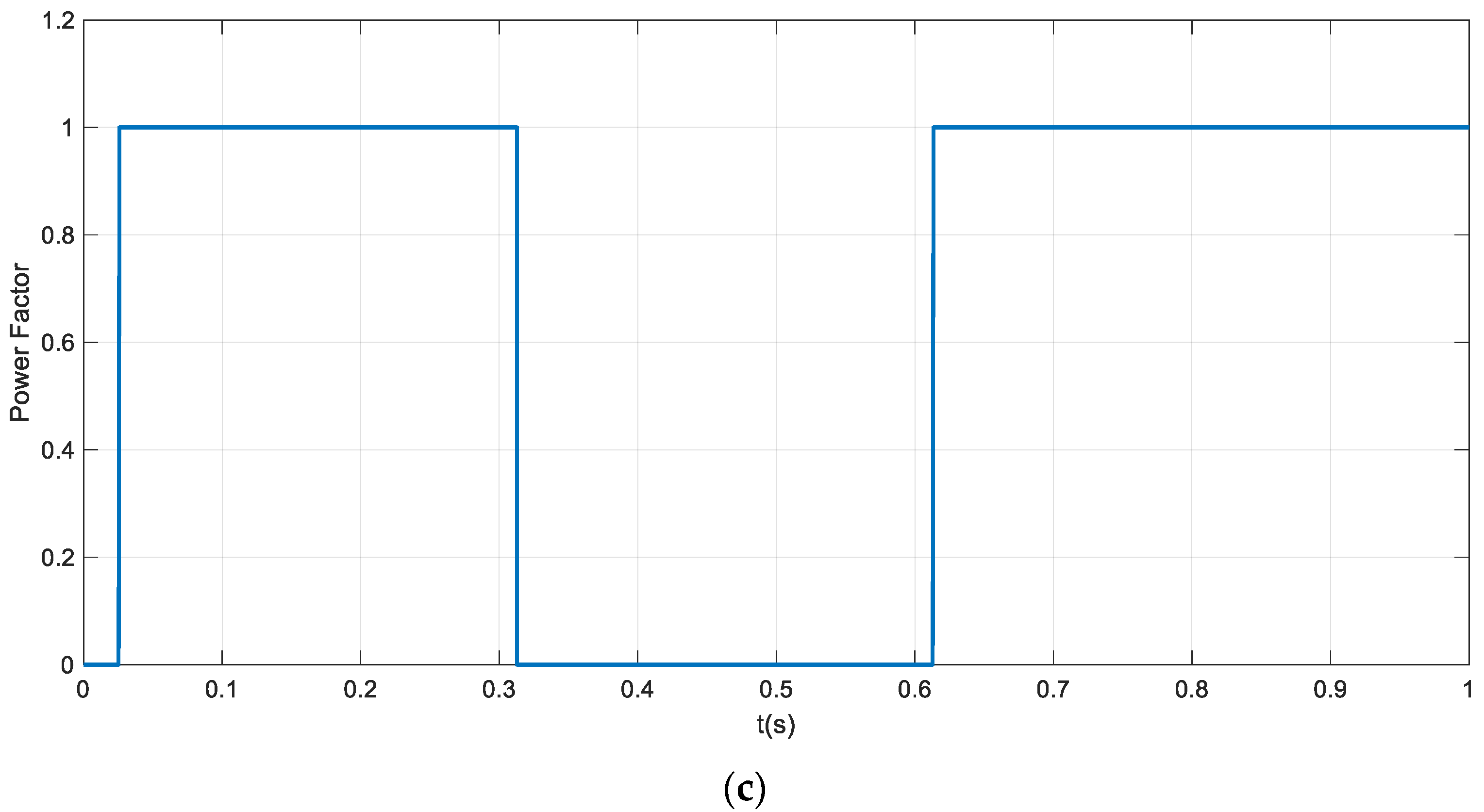
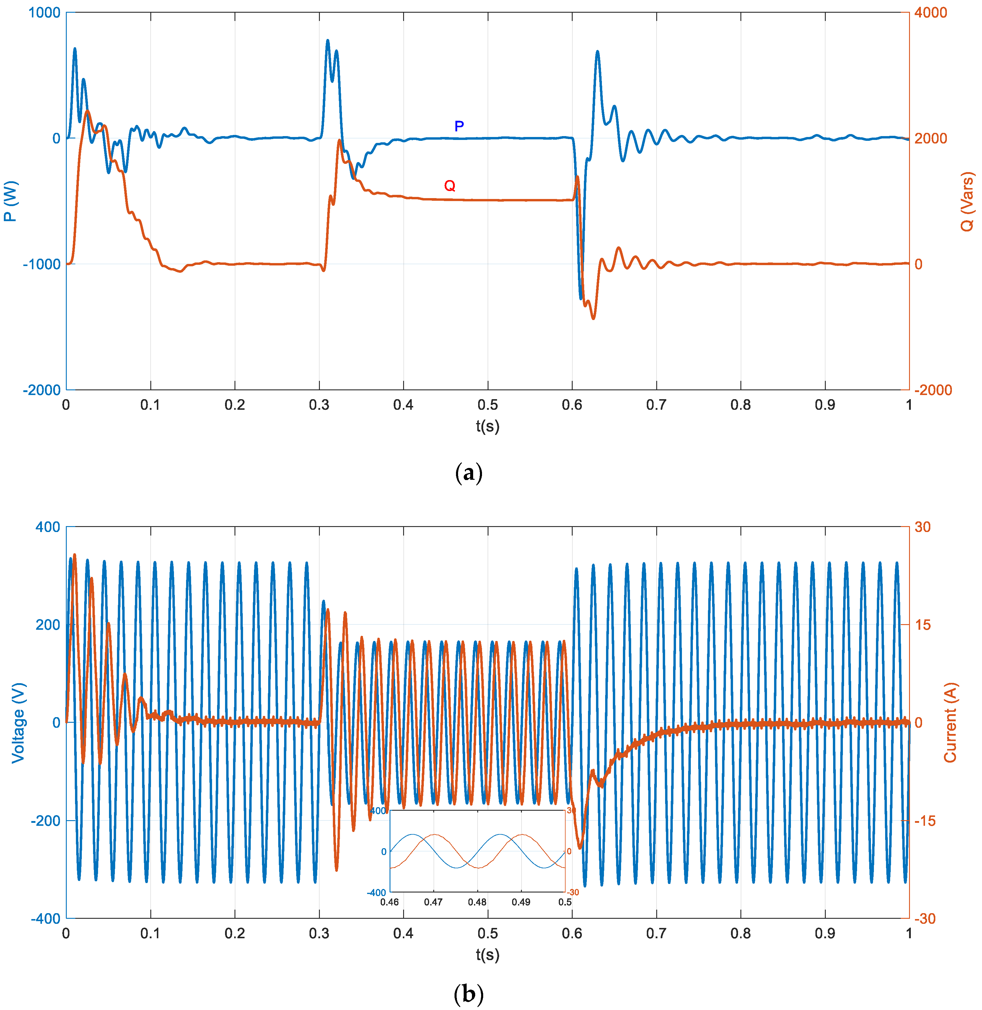
Figure 11, Figure 12 and Figure 13, show, respectively, the night mode results when the grid voltage is at 75%, 50%, and 10% of grid’s nominal voltage value (i.e., voltage sag depth of 25%, 50%, and 90%). Again, simulation results show that zero active power is injected into the grid before and after the voltage sag. On the other hand, the inverter’s reactive power changed from zero to approximately 100% of the rated capacity corresponding to rated current flowing into the grid at 90° leading. Note that reactive power level, in all three cases, is reduced in proportion to the voltage sag, thus allowing close to rated current flow. For example, for 90% voltage sag, the reactive power is very low, since this condition resembles an approximate short circuit condition at the grid side.

4. Conclusions

In this paper, active and reactive power injection for single-phase grid-connected PV system with LVRT capability was explored. Two PI controller and a FLC were used to control the operation of the inverter during normal and faulty operations of the grid-connected inverter. The PI regulators were tasked to regulate the active and reactive power flow according to MPPT settings. However, during faulty operation of the grid, when a voltage sag is detected, the FLC is tasked to recommend a PF for the inverter operation based on the available capacity of the inverter and the voltage sag level. For severe voltage sag levels, the full capacity of the inverter is dedicated to the reactive power compensation and real power is de-rated to zero. On the other hand, whenever a voltage sag of moderate level is detected, the FLC will also use the level of the PV system power; if it is low, the recommended PF value will also be low.

In addition, a PQ calculator was implemented to perform a check to ensure that the inverter’s maximum capacity is always not exceeded. If the capacity is exceeded, the real power will be de-rated using the same PF value obtained from the FLC.

The proposed control scheme showed good performance in terms of accurate control of power flow into grid, detection of voltage sags, and injection of real and reactive power at a selected power factor without exceeding the inverter’s capacity. Further improvements in future studies can include examining alternative types of controllers and methodologies to enhance the transient response of the system, namely the overshoot in active and reactive power responses.

References

- IEA; IRENA; UNSD; WHO. Tracking SDG 7: The Energy Progress Report 2019. Available online: https://irena.org/publications/2019/May/Tracking-SDG7-The-Energy-Progress-Report-2019 (accessed on 15 November 2019).
- Beena, V.; Jayraju, M.; Sebin, K.D. Active and reactive power control of single phase transformerless grid connected inverter for distributed generation system. Int. J. Appl. Eng. Res. 2018, 13, 150–157. [Google Scholar]
- Panda, A.; Pathak, M.K.; Srivastava, S.P. Single Phase Photovoltaic Inverter Control for Grid Connected System. Sadhana 2016, 41, 15–30. [Google Scholar] [CrossRef] [Green Version]
- IEA. Tracking Power, IEA Report, Paris, Paris 2019. Available online: https://www.iea.org/reports/tracking-power-2019 (accessed on 15 November 2019).
- Yang, Y.; Blaabjerg, F. Overview of single-phase grid-connected photovoltaic systems. Electr. Power Compon. Syst. 2015, 43, 1352–1363. [Google Scholar] [CrossRef] [Green Version]
- Arafa, O.M.; Mansour, A.A.; Sakkoury, K.S.; Atia, Y.A.; Salem, M.M. Realization of single-phase single-stage grid connected PV system. J. Electr. Syst. Inf. Technol. 2017, 4, 1–9. [Google Scholar] [CrossRef] [Green Version]
- Golestan, S.; Monfared, M.; Guerrero, J.M.; Joorabian, M. A D-Q Synchronous Frame Controller for Single Phase Inverters. In Proceedings of the 2nd Power Electronics, Drive Systems and Technologies Conference, Tehran, Iran, 16–17 February 2011. [Google Scholar]
- Yang, Y.; Wang, H.; Blaabjerg, F. Reactive power injection strategies for single-phase photovoltaic systems considering grid requirements. In Proceedings of the 29th Annual IEEE Applied Power Electronics Conference and Exposition, Fort Worth, TX, USA, 16–20 March 2014. [Google Scholar]
- KO, S.-H.; Lee, S.-R.; Dehbonei, H.; Nayar, C.V. A grid-connected photovoltaic system with direct coupled power quality control. In Proceedings of the 32nd Annual conference on IEEE Industrial Electronics, Paris, France, 6–10 November 2006. [Google Scholar]
- Taleb, M.; Mansour, N.; Zehar, K. An improved grid tied photovoltaic system based on current conditioning. Eng. Sci. Technol. Int. J. 2018, 21, 1113–1119. [Google Scholar] [CrossRef]
- Sadat, S.; Patel, J. A review of low voltage ride-through capability techniques for photovoltaic power plant systems. Int. J. Tech. Innov. Mod. Eng. Sci. 2019, 5, 633–640. [Google Scholar]
- Benali, A.; Khiat, M.; Allaoui, T.; Denai, M. Power quality improvement and low voltage ride throught capability in hybrid wind-pv farms grid-connected using dynamic voltage restorer. IEEE Access 2018, 6, 68634–68648. [Google Scholar] [CrossRef]
- Sravanthi, Y.; Sujatha, P. Fuzzy logic controller for low voltage ride through capability improvement of grid connected photovoltaic power plants. Int. J. Adv. Res. Electr. Electron. Instrum. Eng. 2017, 6, 7213–7226. [Google Scholar]
- Li, K.; Qian, J.; Wu, H.; Li, T.; Yang, J. Research on low voltage ride through of the grid-connected PV system. In Proceedings of the International Conference on Advances in Energy, Environment and Chemical Engineering, Changsha, China, 26–27 September 2015. [Google Scholar]
- Yang, Y.; Blaabjerg, F. Low-Voltage Ride-Through Capability of a Single-Stage Single-Phase Photovoltaic System Connected to the Low-Voltage Grid. Int. J. Photoenergy 2013, 2013. [Google Scholar] [CrossRef] [Green Version]
- Al-Shetwi, A.Q.; Sujod, M.Z.; Ramli, N.L. A review of the fault ride through requirements in different grid codes concerning pentration of pv system to the electric power network. ARPN J. Eng. Appl. Sci. 2015, 10, 9906–9912. [Google Scholar]
- Zhu, B.; Yang, Y.; Ji, A.; Tao, X.; Xie, M.; Cao, F. A novel control strategy for single-phase grid-connected PV generation system with the capability of low voltage ride through. J. Electr. Syst. 2014, 10, 370–380. [Google Scholar]
- Al-Shetwi, A.Q.; Sujod, M.Z.; Blaabjerg, F. Low voltage ride-through capability control for single-stage inverter-based grid-connected photovoltaic power plant. Sol. Energy 2018, 159, 665–681. [Google Scholar] [CrossRef] [Green Version]
- Mohammadi, P.; Azimian, B.; Shahirinia, A. A Novel Double-Loop Control Structure Based on Fuzzy-PI and Fuzzy-PR Strategies for Single-Phase Inverter in Photovoltaic Application. In Proceedings of the 2018 North American Power Symposium (NAPS), Fargo, ND, USA, 9–11 September 2018. [Google Scholar]
- Islam, S.; Zeb, K.; Din, W.; Khan, I.; Ishfaq, M.; Busarello, T.; Kim, H. Design of a Proportional Resonant Controller with Resonant Harmonic Compensator and Fault Ride Trough Strategies for a Grid-Connected Photovoltaic System. Electronics 2018, 7, 451. [Google Scholar] [CrossRef] [Green Version]
- Radwan, E.; Saleh, K.; Awada, E.; Nour, M. Modified phase locked loop for grid connected single phase inverter. Int. J. Electr. Comput. Eng. 2019, 9, 3934–3943. [Google Scholar] [CrossRef]
- Hadjidemetriou, L.; Yang, Y.; Kyriakides, E.; Blaabjerg, F. A Synchronization Scheme for Single-Phase Grid-Tied Inverters under Harmonic Distortion and Grid Disturbances. IEEE Trans. Power Electron. 2017, 32, 2784–2793. [Google Scholar] [CrossRef] [Green Version]
- Benz, C.H.; Franke, W.-T.; Fuchs, F.W. Low voltage ride through capability of a 5 kW grid-tied solar inverter. In Proceedings of the 14th international Power Electronics and Motion Control Conference, Ohrid, Macedonia, 6–8 September 2010. [Google Scholar]
- Zhang, Z.; Yang, Y.; Ma, R.; Blaabjerg, F. Zero-voltage ride-through capability of single-phase grid-connected photovoltaic system. Appl. Sci. 2017, 7, 315. [Google Scholar] [CrossRef]
- Yao, Z.; Xiao, L.; Guerreo, J.M. Improved control strategy for the three-phase grid-connected inverter. IET Renew. Power Gener. 2015, 9, 587–592. [Google Scholar] [CrossRef] [Green Version]
Figure 1.
Structure of the proposed single-phase grid connected PV system.
Figure 2.
Voltage support requirements under grid faults for wind turbines [15,23]. are grid nominal voltage and current, are the voltage and reactive current before failure, and are the instantaneous voltage and reactive current.
Figure 3.
Fuzzy input and output membership functions.
Figure 4.
Simplified equivalent circuit model: (a) grid-connected inverter simplified equivalent circuit; (b) space vectors of voltages and currents.
Figure 5.
Power angle regulator.
Figure 6.
Inverter voltage regulation.
Figure 7.
Simulation results when the grid voltage drops from nominal value to 75% during day time operation. (a) Injected active and reactive power, (b) voltage and current at PCC, (c) power factor from FLC.
Figure 8.
Simulation results when the grid voltage drops from nominal value to 50% during day time operation. (a) Injected active and reactive power, (b) voltage and current at PCC, (c) power factor from FLC.
Figure 9.
Simulation results when the grid voltage drops from nominal value to 10% during day time operation. (a) Injected active and reactive power, (b) voltage and current at PCC, (c) power factor from FLC.
Figure 10.
Simulation results when the grid voltage drops from nominal value to 75% during cloudy day time operation. (a) Injected active and reactive power, (b) voltage and current at PCC, (c) power factor from FLC.
Figure 11.
Simulation results when the grid voltage drops from nominal value to 75% during night time operation. (a) Injected active and reactive power, (b) voltage and current at PCC, (c) power factor from FLC.
Figure 12.
Simulation results when the grid voltage drops from nominal value to 50% during night time operation. (a) injected active and reactive power, (b) voltage and current at PCC, (c) power factor from FLC.
Figure 13.
Simulation results when the grid voltage drops from nominal value to 10% during night time operation. (a) Injected active and reactive power, (b) voltage and current at PCC, (c) power factor from FLC.