Evaluation Model for the Scope of DC Interference Generated by Stray Currents in Light Rail Systems

1
School of Mechatronic Engineering, China University of Mining and Technology, No. 1 Daxue Road, Xuzhou 221116, China
2
Guangzhou Metro Design & Research Institute Co., Ltd., No. 204 Huanshi West Road, Guangzhou 510030, China
*
Author to whom correspondence should be addressed.
Energies 2019, 12(4), 746; https://0-doi-org.brum.beds.ac.uk/10.3390/en12040746
Submission received: 31 January 2019
/
Revised: 19 February 2019
/
Accepted: 22 February 2019
/
Published: 23 February 2019
Abstract
:Electrochemical corrosion caused by stray currents reduces the lifespan of buried gas pipelines and the safety of light rail systems. Determining the scope of stray current corrosion will help prevent the corrosion of existing buried pipelines and provide an effective reference for new pipeline siting. In response to this problem, in this paper the surface potential gradient was used to evaluate the scope of stray current corrosion. First, an analytical model for the scope of the stray current corrosion combined with distributed parameters and the electric field generated by a point current source was put forward. Second, exemplary calculations were conducted based on the proposed model. Sensitivity of the potential gradient was analyzed with an example of the transition resistance, and the dynamic distribution of surface potential gradient under different locomotive operation modes was also analyzed in time-domain. Finally, the scope was evaluated at four different intervals with the parameters from the field test to judge whether the protective measures need to be taken in areas with buried pipelines and light rail systems nearby or not.

1. Introduction
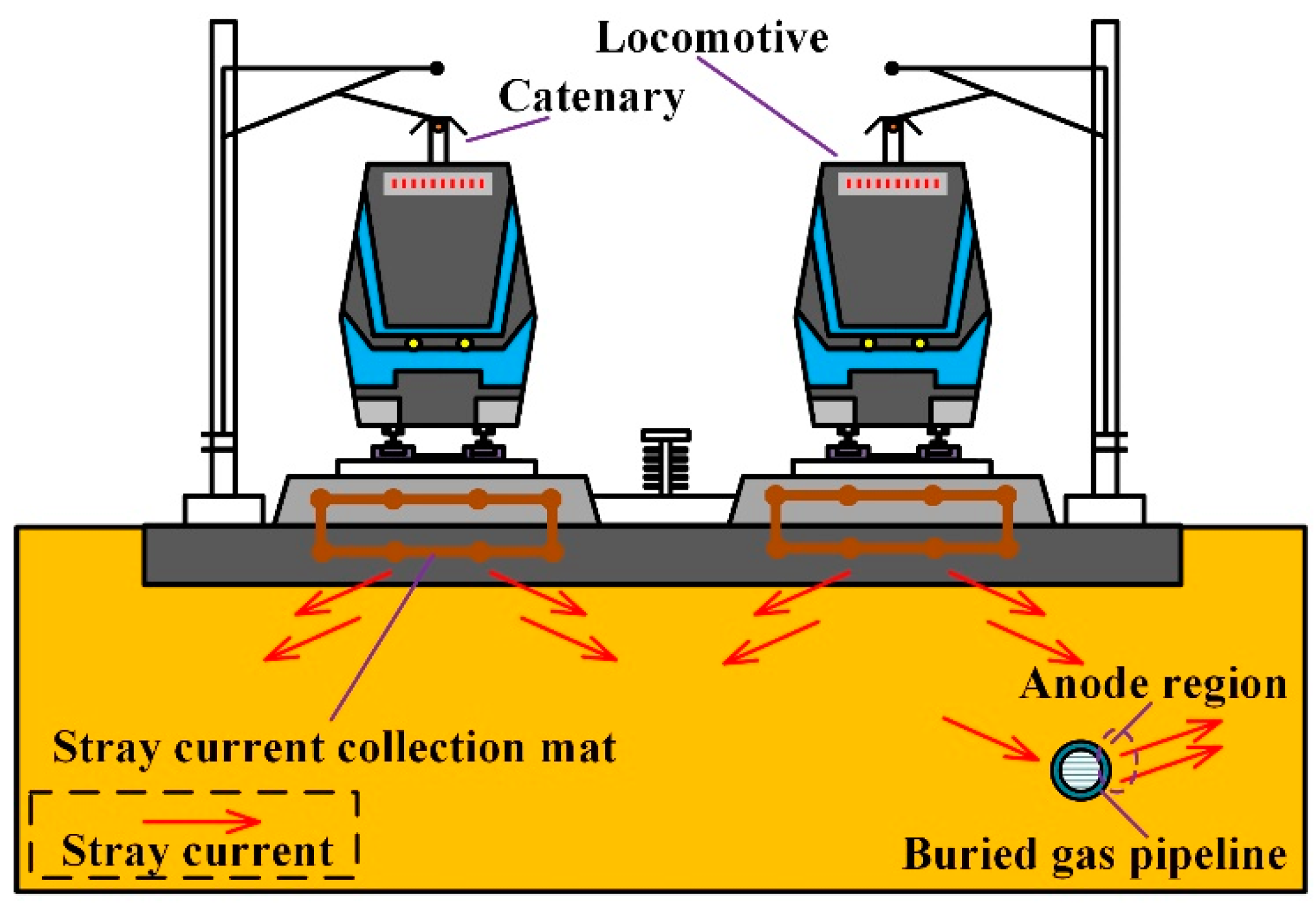
In a light rail system, stray currents deviating from the original return path are generated due to decreasing resistance in some areas and the blocked backflow system [1,2,3,4], which is explicitly shown in Figure 1. Differing from the traction current flowing back to the traction substation along the rails, the stray current will first flow into the underground and then flow back to the negative terminal of the traction substation. The reason for this phenomenon is that the resistance of the target path is greater than the unintended path. In other words, the stray current can occur as a result of potential gradients in the earth. Especially when the transition resistance between the rail and the earth is much lower than the standard value given by the standard after a period of operation, the stray current leakage increases significantly. The AC stray current has been proved to be less dangerous than the DC stray current [5]. In addition to the rise of rail potential [6], the stray current will cause electrochemical corrosion in some of the infrastructure, such as the running rails [7], buried pipelines [8] and concrete structure [9], which overall reduces the safety performance of the light rail system [10]. Three grounding strategies are usually used in the light rail system, which are diode-grounded schemes, directly grounded schemes and ungrounded schemes, respectively [11]. It is known that the earthing scheme carried out in a light rail system influences the stray current distribution. The system with directly-grounded scheme suffers the stray current most seriously while avoids the excessive rail potential [12].
Buried gas pipelines often exist in and around DC light rail systems. Buried gas pipe has good longitudinal electrical conduction, and it easily accumulates currents from a distant place. Stray current corrosion problems accordingly exist on buried gas pipelines, some of which are discovered as pitting corrosion within a few years or even months [13]. In addition, the pipe wall is thin, so it is susceptible to stray current corrosion, and it is necessary to take appropriate prevention measures. The stray current can polarize, either anodically or cathodically, the buried pipelines at the anodic or cathodic zone, respectively. Resulting from the distinguishing environments, the specific reaction equation is diverse, which are oxygen absorption corrosion and hydrogen evolutional corrosion [14,15]. Stray currents are mainly conducted through the soil, and thus their scope of influenc is relatively limited. The analysis of the DC interference scope, in essence, is to determine the scope of the excessive electrochemical corrosion on the buried pipelines caused by a stray current. Due to the complexity of the stray current distribution in a light rail system, it is difficult to analyze the specific flow direction of the stray current in the ground by theoretical modeling. The existing standards clearly define the methods and indexes for identifying stray current disturbances through the surface potential gradient, polarization potential and other parameters [16,17,18,19,20,21]. Therefore, in order to determine the scope of the stray current interference, existing standards can be used to assess the stray current interference in the buried pipelines at different locations. For existing buried gas pipelines buried in a light rail system, it is necessary to analyze the influence range of the stray current in the light rail system to determine the degree of DC interference and provide reference information for additional protection measures, such as cathodic protection. On the other hand, when pipelines are to be embedded around a light rail system, it is necessary to consider the range of influence of the stray currents of the light rail system in the vicinity of the gas pipes, to determine the suitable embedding position and minimize the corrosion effect of the stray current on the buried gas pipelines. Based on these reasons, the research on the DC interference scope is of great significance in the anti-corrosion of buried gas pipelines.
There is a certain amount of foundational research on the 3-dimensional distribution of stray current and the corrosion risk caused by it. Many methods, such as the Earth return model [22], hemispherical electrode model [23], CEDGS simulation [24,25], FEM [26] and Simulink simulation [27] are proposed or used to study this topic. The main objective of this paper is to provide a scope model of the DC interference evaluated by the surface potential gradient. In this paper, the surface potential gradient is chosen as a parameter to characterize the DC interference scope, which is easy to measure in practical engineering application. The evaluation model of the DC interference scope is proposed, and the exemplary calculations are given. Compared with the existing research results, the model proposed in this paper can evaluate stray current disturbances on a buried pipeline near a light rail system more directly. The results of this paper are of theoretical significance for the corrosion protection of buried gas pipelines affected by stray currents. The rest of this paper is organized as follows: Section 2 introduces the mathematical model. Exemplary calculations are performed and discussed in Section 3. The evaluation of DC interference scope based on field tests is presented in Section 4. Finally, conclusions are drawn in Section 5.
2. Mathematical Model
2.1. Research Background and an Overview of the Model
Many standards reguklate the methods for identifying the DC interference caused by the stray currents. For example, four principal methods for identifying stray current interferences are provided in EN 50162-2004, among which the voltage gradients in the electrolyte are included [17]. Similarly, it is stated in GB/T 19285-2003 that DC interference exists when the surface potential gradient is above 0.5 mV/m and some special measures, such as drainage protection or cathodic protection, should be taken when the surface potential gradient near the buried pipelines is above 2.5 mV/m [16]. In NACE SP0207-2007, procedures for the surface potential gradient surveys is presented [21], which is used to DC surface potential gradient surveys on buried or submerged metallic pipelines is provided. The surface potential gradient ruled in the standard GB/T 19285 provided the minor and major corrosion risk no matter how deep the pipeline is buried [16].
In view of this, the evaluation model is designed to evaluate the scope of DC interference caused by stray currents using the surface potential gradient. The model is used to judge whether the area around the light rail system is influenced by the stray current corrosion or not using the surface potential gradient. The model is also used to provide references to decide whether protective measures should be taken or not. The surface potential gradient is calculated through the stray current distribution and the potential generated by the injected current at one point, which is a part of the stray current leakage. Finally, the threshold value 2.5 mV/m and 0.5 mV/m from GB/T 19285-2003 is used to judge whether the protective measures need to be taken in the area with buried pipeline and light rail system nearby or not.
2.2. Earth Potential Generated by the Point Current Source
Since the stray current leakage in the supply interval is composed of current leaked from each point to the Earth, the Earth potential generated by a point current source should be further calculated under the premise of stray current leakage along the running rail. In a cylindrical coordinate system, the current field generated by a point current source in uniformly distributed soil can be obtained by solving the Laplace differential equation for a given boundary condition:
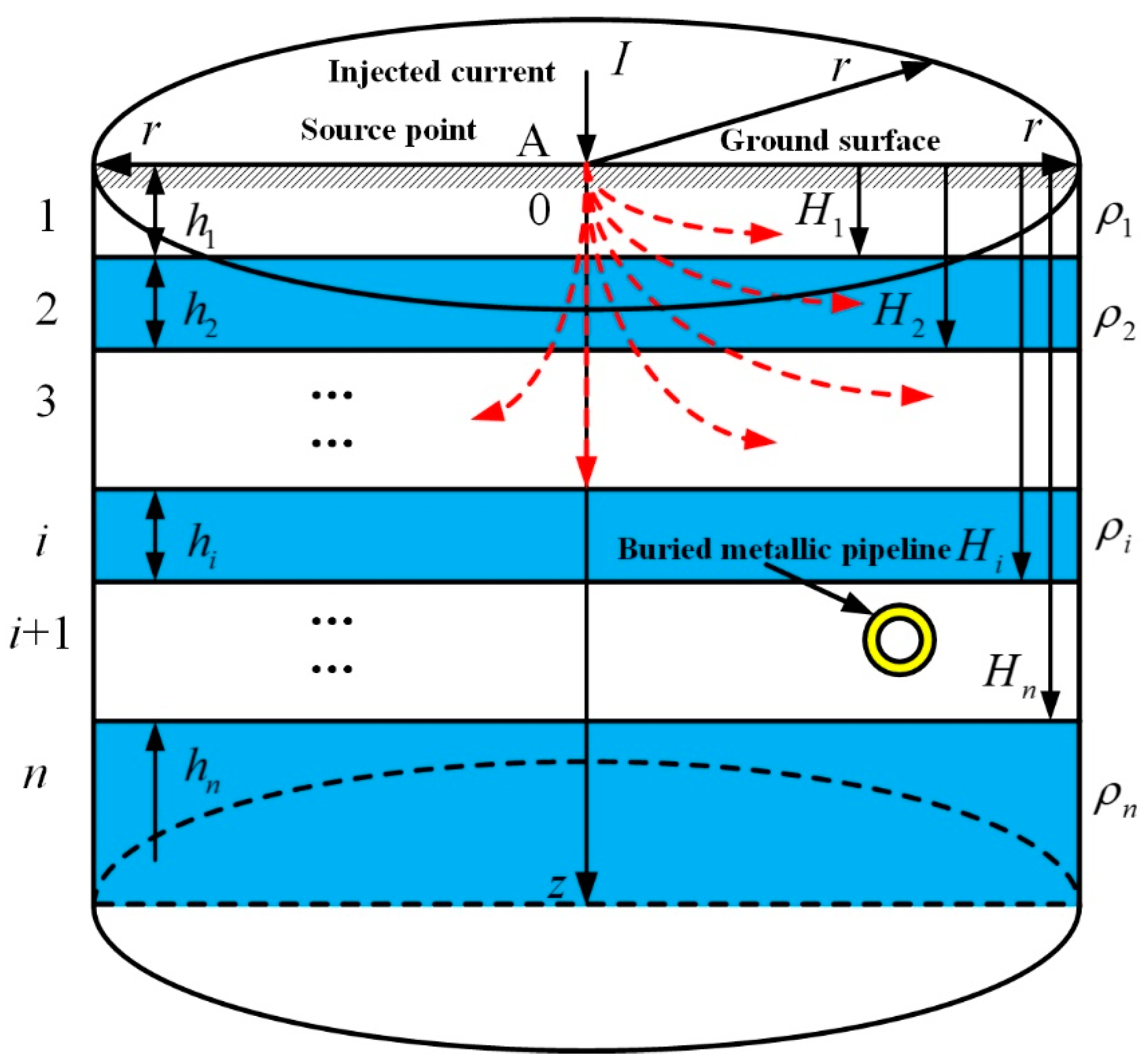
The n layers of a horizontal layered structure underground are shown in Figure 2. The resistivity of each layer is ρ1, ρ2, …, ρn and the thickness of each layer is h1, h2, …, hn. The distance from each interface to the ground surface is H1, H2……, Hn. A point current source with a current intensity I is injected at point A on the ground surface. The variable separation method is used to solve Equation (1), which can be derived as:
where J0(λr) is the zeroth-order Bessel function, and Ai(λ) and Bi(λ) are the functions of the integral variable λ.
Furthermore, the potential of the first layer in the soil can be regarded as having two parts: one is the potential generated by the point current source in the semi-infinite medium and the other is the solution of the Laplace differential equation. Therefore, the potential of the first layer is given by:
where h is the depth of the current source in meters.
When the depth tends to infinity, the potential is considered to be zero. Thus, the first boundary condition can be given as:
On the ground surface of the top layer, the upper layer of the medium is air, the resistivity of which is infinite. The second boundary condition is:
Assuming that the soil model is a simple distribution of one layer, the potential can be decided by solving the coefficients A1(λ) and B1(λ) in Equation (6):
Equation (6) can be furtherly simplified by the Lipschitz integral. The return rail is considered to be placed at the ground surface so that the current source depth h in Equation (6) is zero.
2.3. Surface Potential Gradient Near the Running Rail under the Stray Current Leakage
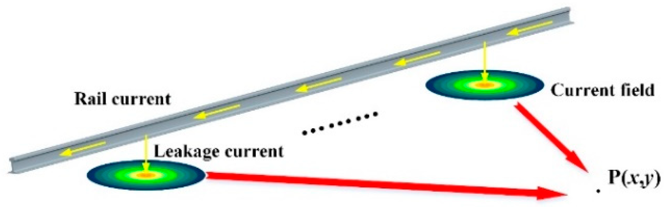
Supposing that there is a point P on the ground surface near the running rail whose coordinates are (x, y). According to the potential derived in Section 2.2, the potential at point P is affected by the current leaking into the Earth at each point along the running rail through the current field, which can be expressed mathematically as the integration of the potential produced by all the stray current leakage points at point P, as shown in Figure 3.
Depending on the research results obtained by Li [28] and Xu [3], the stray current and rail potential based on the running rail-buried metallic pipeline-Earth structure under the bilateral power supply can be derived. Thus, the leakage current over length dm can be indicated as:
where Rg is the transition resistance between the running rails and Earth, assumed uniform, in Ω·m; u(x) is the rail potential at x in volts, which is at the middle of the dm.
In consequence, the ground surface potential at point P produced by a stray current under the unilateral power supply can be determined from the expression:
In combination with the resistive network model and the above method, the surface potential gradient at point P produced by a stray current under the bilateral power supply is given as:
where α and Z are the intermediate variable for more concise representation; RS is the rail longitudinal resistance, assumed uniform, in Ω/km; RR is the longitudinal resistance of the buried metallic pipeline, assumed uniform, in Ω/km; L1 is the distance from the locomotive to the substation in kilometers; L is the distance of the traction interval in kilometers; ρ is the soil resistivity in and near the power supply interval, assumed uniform, in Ω·m, and I0 is the traction current in amperes.
The potential gradient is defined in Equation (10):
Under the bilateral power supply, the surface potential gradient near the running rail can be obtained by substituting Equations (9) and (10) into Equation (11):
In the range of 0 to L1, the partial derivative of the surface potential for the variables x and y can be found in Equations (A1) and (A2) of Appendix A. In the range of L1 to L, the partial derivative of the surface potential for the variables x and y can be found in Equations (A3) and (A4) of Appendix A.
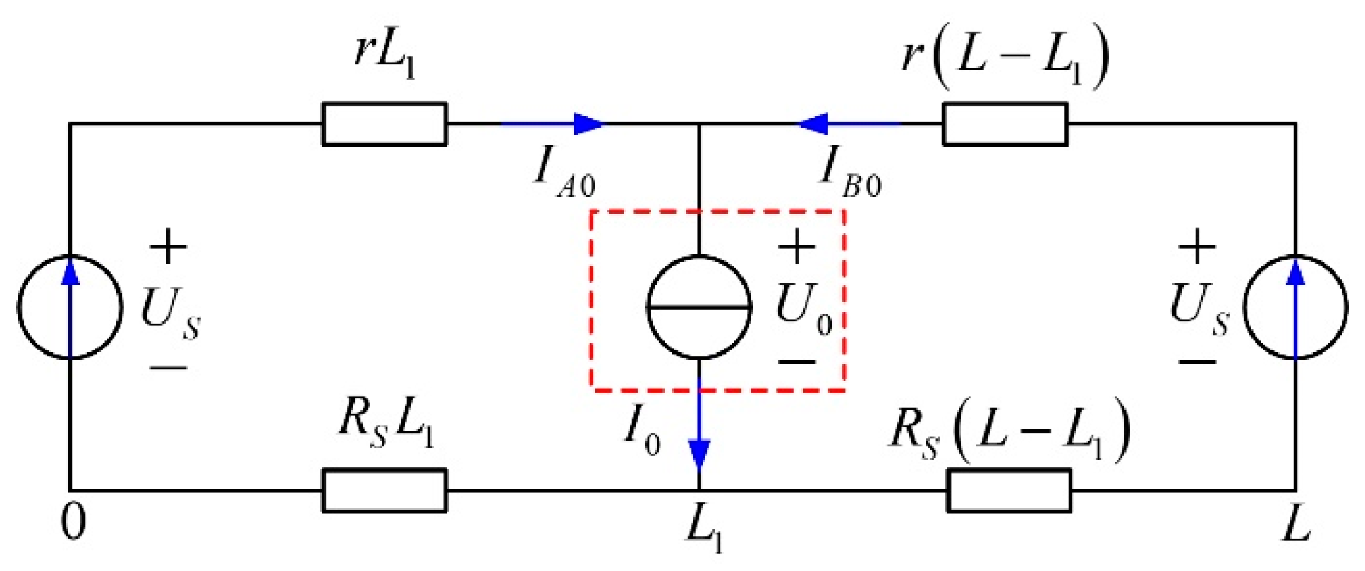
In addition, the evaluation model is built up in time-domain considering the moving locomotive and time-varying current. The locomotive is equivalent to an ideal current source, and the substations are regarded as the ideal voltage source. The powered equivalent model is shown in Figure 4. According to Kirchhoff’s law, the traction current from two substations are given as the Equations (13) and (14):
where P is the power of locomotive in light rail systems in kilowatts. US is the traction substation voltage in volts. r is resistance of catenary, assumed uniform, in Ω/km.
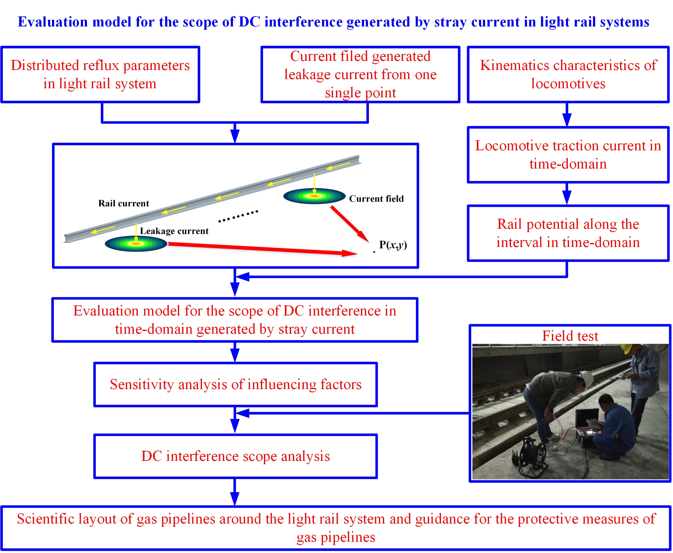
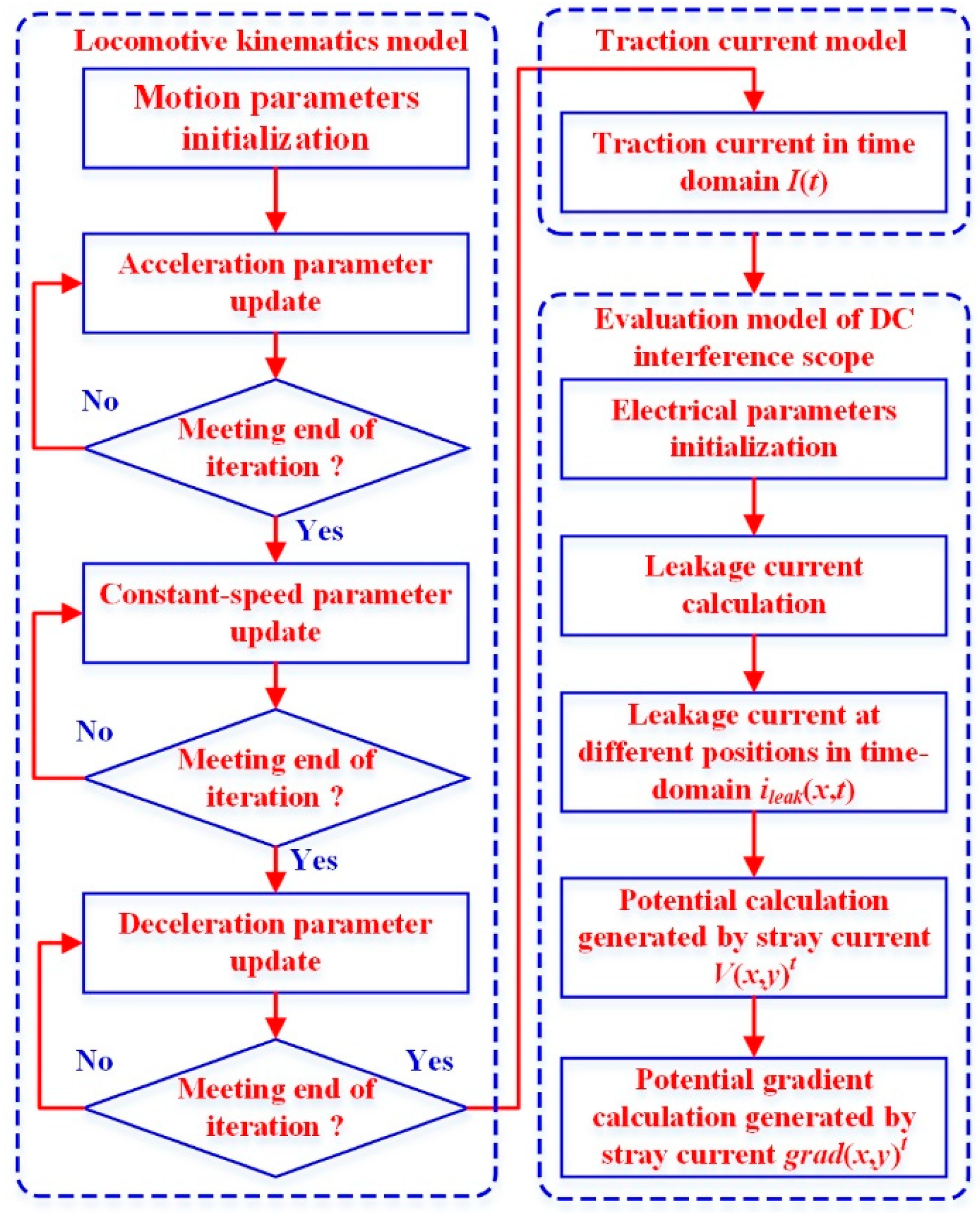
The traction current I0(t) = [I01, I02, I03, …, I0t, …, I0T], locomotive power P(t) = [P1, P2, P3, …, Pt, …, PT] and corresponding position of locomotive S(t) = [S1, S2, S3, …, St, …, ST], is calculated first with the time interval Δt, 0 < t < T, T is the entire operation time. Then the rail potential along the whole interval is determined with different operation time u(x,t). The leakage current ileak(x,t) at any position within the operation time is obtained. Based on the evaluation model, the potential V(x,y)t generated by the stray current is calculated in the current field. Finally, the surface potential gradient grad(x,y)t is obtained according to the potential distributing. The whole calculation flow is shown in Figure 5.
3. Exemplary Calculations
3.1. Calculation Parameters
Next, the exemplary analysis is conducted according to the surface potential gradient model. The parameters deemed necessary for the exemplary calculations are shown in Table 1. The soil resistivity is measured using the Wenner method near the light rail system.
3.2. Surface Potential Gradient under the Bilateral Power Supply
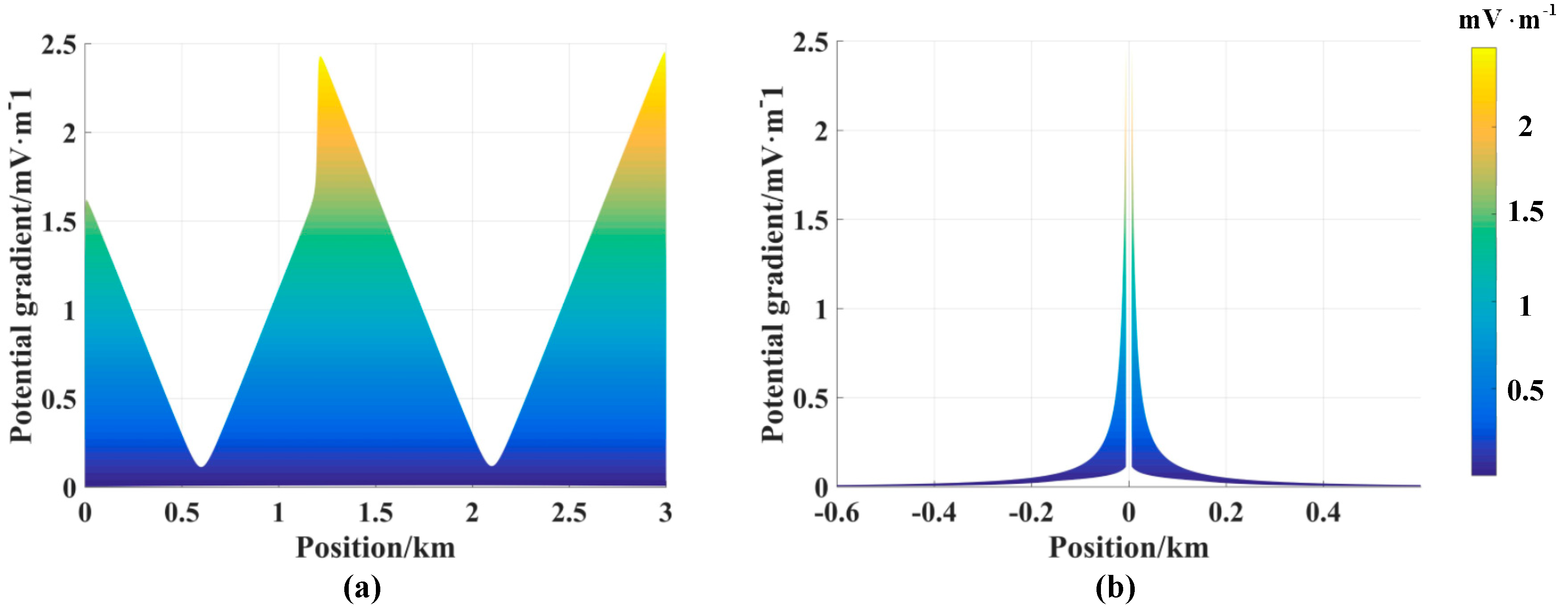
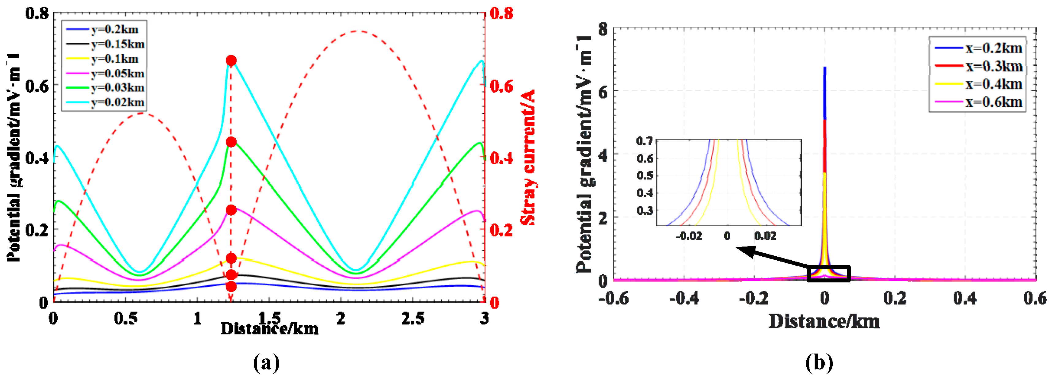
It is assumed that the locomotive is 1.2 km away from the substation within the interval, and the surface potential gradient near the running rail under the bilateral power supply is illustrated in Figure 6. The surface potential gradient at different positions is shown in Figure 7.
It can be observed that the surface potential gradient is symmetrically distributed both along the locomotive running direction and reaches a maximum both near the locomotive and the traction substation under the bilateral power supply.
The ultimate consequence of DC interference is stray current corrosion on nearby buried gas pipelines. Thus, pipelines arranged near substations are more likely to be affected by stray current corrosion, and pipelines are more likely to be affected by stray current corrosion when the locomotive is nearby. The reason for this is that the greater potential gradient means larger amount of potential change per unit length, which causes larger stray current flowing in the electrolyte. According to the Faraday’s first law, the mass of the chemically altered substance at the electrode interface is proportional to the amount of electricity supplied. It can be expressed as Equation (15), where M is molar mass of the metal in g/mol, n is the valency, F is the Faraday constant, t is the corrosion time in seconds and i is the current flowing out of the anode metal in amperes. That is to say, larger potential gradient leads to greater corrosion within the same period. The distribution of stray current is also shown in Figure 7. The entire internal traction is divided into two parts according to the locomotive position. The length of interval A is 1.2 km, while the length of interval B is 1.8 km. The stray current reaches a maximum value in the two intervals A and B, while it is lowest at the locomotive position. However, the potential gradient is highest at the locomotive position and near the substation. It can be summarized from Figure 7 that the surface potential gradient in interval B is larger than that in interval A. That is, the part of the interval with a longer length suffers more stray current corrosion risk than the part with shorter length. The reason for this phenomenon is that the locomotive requires more traction current from the part of the interval with a longer length than from the part with a shorter length, which will cause a larger surface potential gradient due to more stray current leakage:
The surface potential gradient simulated by COMSOL 5.2 is shown in Figure 8. The simulation parameters are the same as the calculation parameters. The meshing method used in the simulation is free tetrahedral mesh. There are 32,239,340 vol elements, 373,804 surface elements and 13,916 line elements totally. Three following dominant equations are utilized in the SOMSOL simulation. In the homogeneous and isotropic electric field, e.g., soil, concrete, etc., the potential distribution φ is governed by the Laplace Equation (16). The stray current distributed in the soil meets the Ohm’s law as Equation (17). In Equation (17), represents the electric field intensity at any point in the electric field, which is equal to the negative value of the potential gradient at this point. σ is the conductivity of the electrolytes in S/m; is the current density vectors caused by the external current in A/m2; is the current density vectors of the electrolytes. Electrolytes of the interface meet the charge conservation law given by Equation (18), where ie represents the total intensity of stray currents flowing through the electrolyte:
The simulated results show similar trends with the calculated results from the proposed model. It can also be concluded from the simulated results that the buried pipeline will suffer more corrosion hazard at the substations and around the locomotive. The difference between the evaluation model and simulated results is due to the simplification in the running rail-buried metallic pipeline-Earth model, which is a resistive network model to calculate the leakage current from the running rail. In the resistive network model, the soil underground is simplified to a resistive network, which will cause the biases between analytical results and actual situation.
3.3. Impact Factors of the Surface Potential Gradient (Taking the Transition Resistance as an Example)
The nature of the surface potential gradient comes from the stray current leaking from the running rail to the Earth. To analyze the factors of the surface potential gradient, it is necessary to start with the factors of the stray current leakage.
The main factors influencing the stray current include rail-to-Earth transition resistance, longitudinal rail resistance, distance between traction substations, and longitudinal resistance of buried metallic structures. According to the research conducted by Li, the rail-to-Earth transition resistance shows the greatest influence on the stray current leakage [28]. In addition to the transition resistance, the same parameters as in Section 3.2 were adopted. The surface potential gradient with transition resistance from 15 Ω·km to 3 Ω·km are given in Figure 9.
As seen from Figure 9, the surface potential gradient increases with a decrease in the transition resistance, which is consistent for both supply conditions. When the transition resistance decreases from 15 Ω·km to 3 Ω·km, the surface potential gradient increases. However, the surface potential gradient increases less when surface potential gradient is analyzed 200 m away from the rail. While the surface potential gradient also increases with the decreasing transition resistance vertical to the direction of the locomotive. With an increase in the distance from the running rail, the distribution of the surface potential gradient tends to be smoother along the locomotive running direction. With a low transition resistance, not only does the stray current corrosion risk of buried pipelines increase but also the corrosion degree along the entire pipeline is uneven, meaning there is large local corrosion damage.
The surface potential gradient is also influenced by other factors, such as the rail longitudinal resistance, the longitudinal resistance of the buried metal structure, the distance between substations, traction current, etc. The stray current is slightly affected by the longitudinal resistance of the buried pipeline, and thus the surface potential gradient is less likely to be affected by the longitudinal resistance of the buried pipeline. For a reduction in the DC interference scope caused by stray current, it is difficult to change both the material of the buried pipelines and the distance between the substations during the operation of a DC light rail system. Therefore, these factors are not analyzed in this paper. The effect of the traction current on the surface potential gradient is analyzed in detail together with locomotive operating conditions in Section 3.4.
3.4. Dynamic Surface Potential Gradient Considering Locomotive Operation Modes
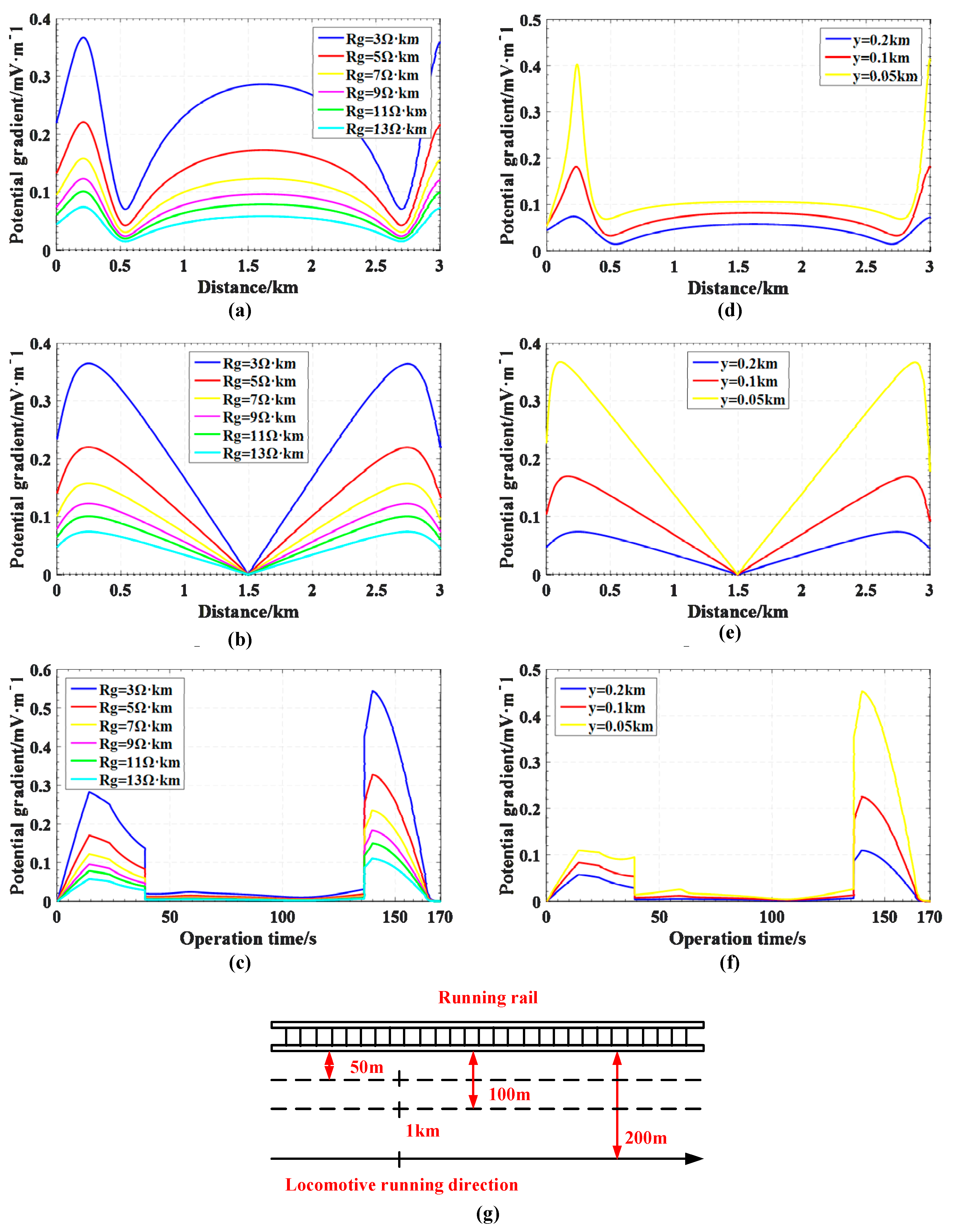
Due to different resultant force, a light rail locomotive generally experiences three different modes from start to braking: acceleration, constant-speed and deceleration. Under these different operation modes, the traction current of the locomotive differs. Based on the theoretical model in Section 2, the surface potential gradient is affected by the traction current and the locomotive location. The two above aspects determine the surface potential gradient near the running rail is time-varying when different operation modes are considered. With the exception of the traction current, the same parameters were applied. The locomotive parameters come from the Metro. The traction current and the locomotive position within a single interval are presented in Figure 10. The acceleration mode is from 0 s to 39 s. The constant-speed mode is from 39 s to 136.2 s. The deceleration mode is from 136.2 s to 170 s.
According to the traction current and the locomotive in the interval, taking the position at a distance of 200 m from the running rail, the surface potential gradient during the starting and braking phase is illustrated in Figure 11a,b, respectively. At a distance of 200 m from the running rail, the surface potential gradient at some point during the entire locomotive operation is presented in Figure 11c. The results and discussion are now carried out. In the deceleration mode, the surface potential gradient near both ends of the interval is higher, so the corrosion risk is enlarged. In the constant-speed mode, the surface potential gradient over the entire interval is low, so the corrosion risk is relatively small. This is because the traction current is only used to generate the same traction force as the operational resistance during the constant-speed period. Compared with the acceleration and the deceleration, only a low traction current is enough to maintain at a constant speed. Therefore, the surface potential gradient is low due to the less stray current leakage. As seen from Figure 11c, the surface potential gradient in the deceleration mode is higher than that in the acceleration mode. The buried pipelines suffer a more serious corrosion risk during the deceleration phase. Because of the need for stopping in a short period of time and the regenerative braking, a large amount of reversed traction current is absorbed, which produces a high surface potential gradient in the interval. Since the traction current flows in the opposite direction to the acceleration mode at this moment, the buried pipelines suffer oxygen evolution corrosion near both substations and suffer hydrogen evolution corrosion near the locomotive. Combining Figure 11b,c, the surface potential gradient in the middle section of the interval is lower overall and less susceptible to stray current corrosion during the three periods of locomotive operation.
With these operation modes considered, the sensitivity analysis of the surface potential gradient is now conducted. The transition resistance and the distance from the running rail are chosen for analysis. For different transition resistances, the surface potential gradient along the locomotive running direction is shown in Figure 12a,b at 100 m and 200 m from the running rail. The surface potential gradients at 25 s and 80 s are shown in Figure 12d,e for different distances from the running rail, respectively. The surface potential gradient within the entire operation time is illustrated in Figure 12c,f.
From Figure 12a,b, it can be observed that the transition resistance significantly influences the dynamic characteristics of the surface potential gradient. Meanwhile, the change in the surface potential along the locomotive running direction gradually decreases with an increase in the transition resistance. As seen from Figure 12d, during the deceleration mode, as the distance from the running rail decreases, the surface potential gradient near both ends of the interval is gradually higher than that in the middle section. During the deceleration mode, the stray current leads to a greater corrosion hazard on the buried pipelines near the running rail at both ends of the interval. It can be seen from Figure 12d–f that the change of the surface potential gradient tends to increase as the distance from the track decreases.
4. DC Interference Scope
On the basis of the potential gradient model indicated in Section 3, as well as the threshold elaborated above, the DC interference scope is further analyzed. In this section, the interference scope of four different traction intervals from light rail line, with different transition resistance and soil resistivity, are calculated and evaluated. The length of these four intervals are 2.97 km, 2.98 km, 2.12 km and 2.23 km, respectively.
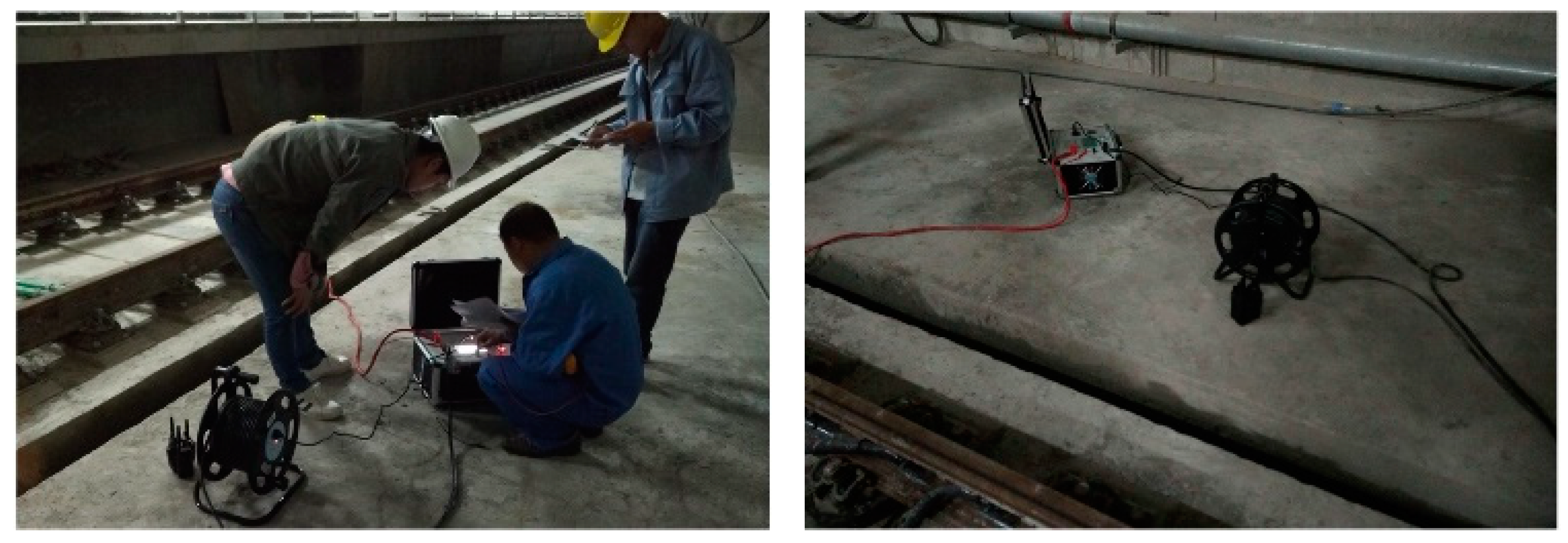
Field tests on the transition resistance and rail longitudinal resistance were conducted in the traction intervals, as shown in Figure 13. The soil resistivity was also tested by the Wenner method accordingly near the different intervals. Each test of transition resistance, rail longitudinal resistance and soil resistivity was repeated 20 times.
The test results, shown in Table 2, are used to evaluate the interference scope furtherly. The MSE of transition resistance, rail longitudinal resistance and soil resistivity is shown in Table 3. The range of soil resistivity test results is greater than the rail-to-earth transition resistance and rail longitudinal resistance. Based on the MSE calculation results, the measurement results are reliable.
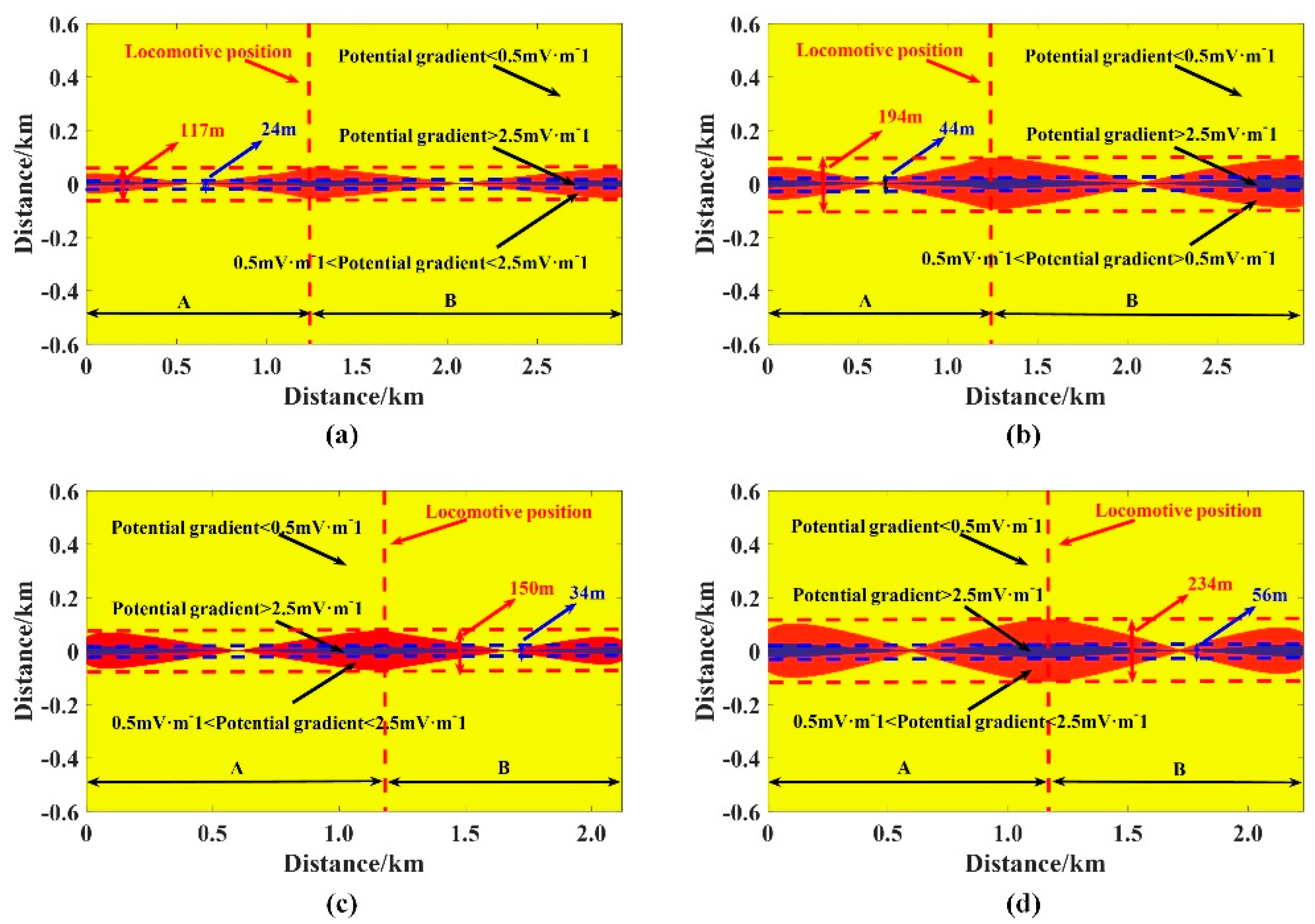
The stray current interference scope is shown in Figure 14 at four different traction intervals. The yellow area in Figure 14 represents that the surface potential gradient is below 0.5 mV·m−1, while the surface potential gradient is between 0.5 mV·m−1 and 2.5 mV·m−1 in the red part of the area in Figure 14. The blue area in Figure 14 shows that the surface potential gradient is above 2.5 mV·m−1.
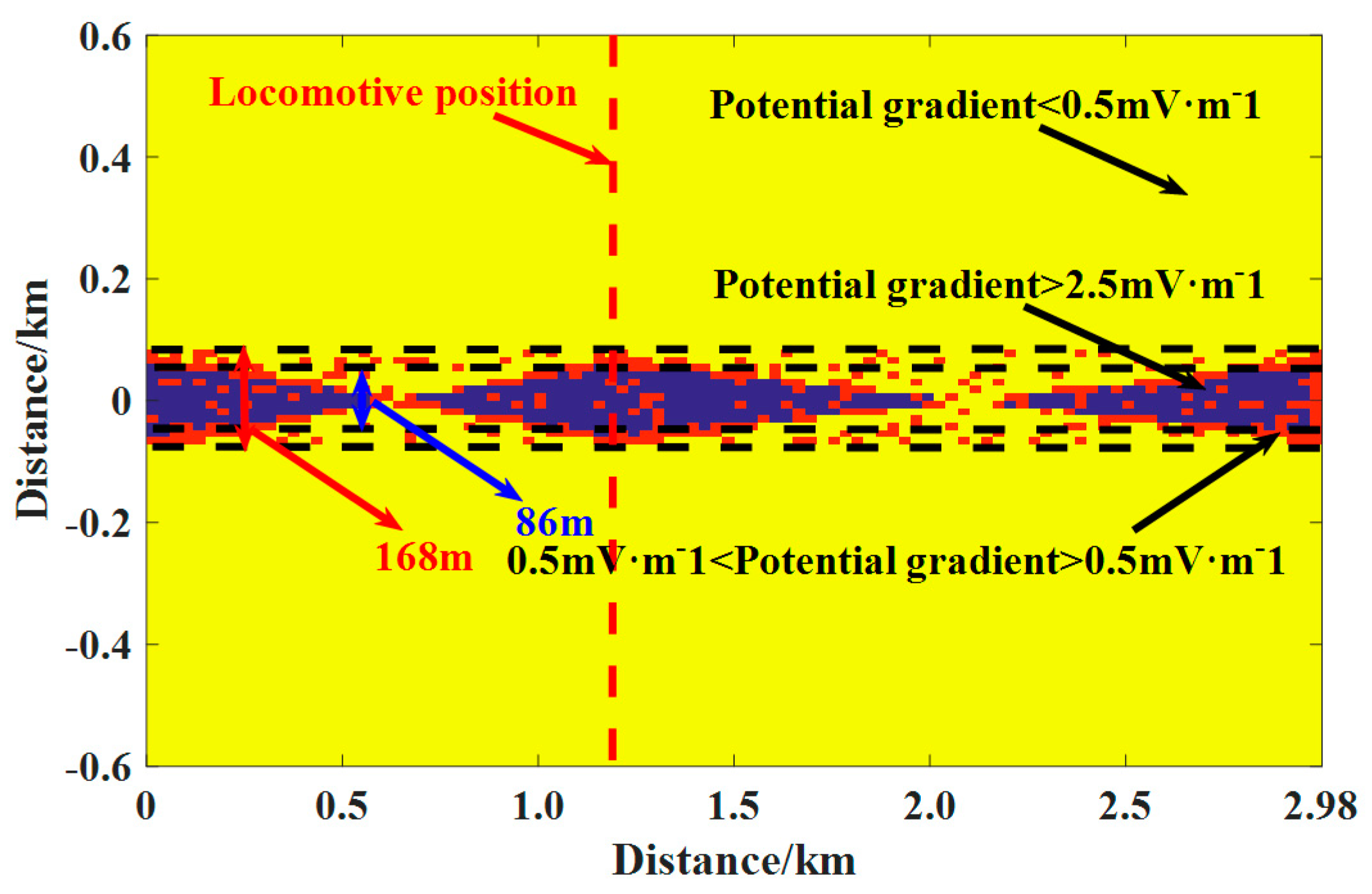
It can be observed from Figure 14a that when the DC interference scope is evaluated at the interval I, the stray current is present within a maximum range of 117 m on both sides of the track and the protective measures need to be applied only within a maximum range of 24 m. When the DC interference scope is analyzed at the interval II, the range that stray current exists in extends to 194 m, while the range where protective measures need to be taken extends to 44 m. As can be observed from Figure 14c, the stray current is present within 150 m on both sides of the running rail at the interval III. Protective measures should be adopted within 264 m on both sides of the running rail in this interval. Finally, the stray current is considered to be existed within a maximum range of 234 m and on both sides of the track at the interval IV, and preventive measures should be taken within a maximum range of 56 m. It can be seen from these four intervals that the traction section with higher traction resistance suffers less stray current corrosion hazard. The DC interference scope at the interval II simulated by COMSOL 5.2 is shown in Figure 15. The area where protective measures need to be taken is bigger than the theoretical result, which is 86 m. And the stray current is existed within a maximum range of 168 m.
5. Summary and Conclusions
(1) In this paper, a time-domain model for evaluating the DC interference scope was proposed and exemplary calculations were conducted. In addition, the DC interference was assessed and calculated, and the distribution characteristics under different operation modes were determined. Based on the field test results in this paper, under a bilateral power supply with four different traction intervals from Metro Line, the maximum range that a severe stray current exists is 117 m, 194 m and 150 m and 234 m on both sides of the track and the maximum range protective measures needs to be taken is 24 m, 44 m and 34 m and 56 m on both sides of the track, respectively.
(2) Under the circumstance provided in this paper, the buried pipelines near substations and the locomotive suffer more DC interference from stray currents, both for a unilateral and bilateral power supply. In other words, these regions are more susceptible corroded by stray current. For the bilateral power supply, if the interval is divided into two parts according to the locomotive position, the DC interference on the buried pipelines caused by stray current is greater in the longer section. That is to say, the stray current corrosion hazard is greater.
(3) The dynamic surface potential gradient was analyzed considering locomotive operation modes. In the acceleration mode, the buried pipelines near the running rail at both ends of the interval are more easily corroded by the stray current. In the deceleration mode, the buried pipelines at both ends of the interval are more easily corroded. In the constant-speed period, the corrosion hazard within the entire interval is quite small. From another point of view, the buried pipelines are more easily corroded in the deceleration mode than the acceleration mode, which has been verified in Section 3.4.
(4) Through the model of the DC interference scope based on the surface potential gradient, the area where corrosion prevention should be emphasized is in the vicinity of substations. When the locomotive brakes, drainage measures need to be enhanced near the substations. If the buried gas pipelines are close to the substations, the monitoring of corrosion risk parameters and the cathodic protection measures should be strengthened. The gas pipelines to be buried immediately after the site selection should avoid passing through the substations to reduce the stray current interference. This model is helpful for scientific layout of gas pipelines around the light rail system in order to avoid DC interference.
(5) However, limitations still exist in the proposed model. The parameters like soil resistivity, transition resistance and rail longitudinal resistance are not constant in and around light rail systems. In this paper, they were all assumed to be homogeneous. Meanwhile, soil topology underground is horizontal distributed with multiple layers. In the proposed model, only one soil layer is considered. These above reasons lead to the limitation of practical applications in the light rail system. In view of this, future work will focus on the modeling of DC interference scope based on non-uniform parameters.
Author Contributions
C.W. wrote the paper and designed the evaluation model; W.L. analyzed the different operation mode of light rail locomotive; Y.W. contributed to the conception of this study; S.X. analyzed the simulation data from the evaluation model; K.L. conducted the field test of simulation parameters and analyzed the experimental data.
Acknowledgments
The authors acknowledge the finance supported by Outstanding Innovation Scholarship for Doctoral Candidate of “Double First Rate” Construction Disciplines of CUMT and Priority Academic Program Development of Jiangsu Higher Education Institutions (PAPD) for this research.
Conflicts of Interest
The authors declare no conflict of interest.
Nomenclature
| h | Depth of the current source | ρ1, ρ2, …, ρn | Soil resistivity in different soil layers |
| h1, h2, …, hn | Thickness of different soil layers | H1, H2, …, Hn | Distance from different interface to the ground surface |
| I | Leakage current from a single current source | Rg | Transition resistance between running rail and earth |
| Rs | Rail longitudinal resistance | RR | Longitudinal resistance of the buried metallic pipeline |
| ρ | Soil resistivity | I0 | Total traction current |
| L | Distance of the traction interval | L1 | Distance from the locomotive to the substation |
| grad(x,y) | Surface potential gradient generated by a single current source | V(x,y) | Surface potential generated by a single current source |
| IA0 | Traction current obtained from substation A | IB0 | Traction current obtained from substation B |
| US | Traction substation voltage | r | Resistance of catenary |
| P | Power of locomotive in light rail systems | Δt | Time interval in exemplary calculation |
| U(x,t) | Rail potential in operation time t | ileak(x,t) | Leakage current in operation time t |
| V(x,y)t | Surface potential in operation time t | grad(x,y)t | Surface potential gradient in operation time t |
| M | Molar mass of the metal | n | Valency |
| F | Faraday constant | t | Corrosion time |
| i | Current flowing out of the anode metal |
Appendix A
When the integral point is between 0 and L1, the partial derivative of x and y in Equation (9) is shown in Equations (A1) and (A2).
When the integral point is between L1 and L, the partial derivative of x and y in Equation (10) is shown in Equations (A3) and (A4):
References
- Li, W.; Yan, X. Research on integrated monitoring and prevention system for stray current in metro. Int. J. Mining Sci. Technol. 2001, 11, 221–228. [Google Scholar]
- Chen, Z.; Koleva, D.; Breugel, K.V. A review on stray current-induced steel corrosion in infrastructure. Corros. Rev. 2017, 35, 397–423. [Google Scholar] [CrossRef]
- Xu, S.; Li, W.; Wang, Y. Effects of vehicle running mode on rail potential and stray current in dc mass transit systems. IEEE Trans. Veh. Technol. 2013, 62, 3569–3580. [Google Scholar]
- Charalambous, C.A.; Cotton, I. Influence of soil structures on corrosion performance of floating-DC transit systems. IET Electr. Power Appl. 2007, 1, 9–16. [Google Scholar] [CrossRef]
- Bertolini, L.; Carsana, M.; Pedeferri, P. Corrosion behavior of steel in concrete in the presence of stray current. Corros. Sci. 2006, 49, 1056–1068. [Google Scholar] [CrossRef]
- Du, G.; Zhang, D.; Li, G.; Wang, C.; Liu, W. Evaluation of rail potential based on power distribution in DC traction power systems. Energies 2016, 9, 729. [Google Scholar] [CrossRef]
- Hernández, F.C.R.; Plascencia, G.; Koch, K. Rail base corrosion problem for north American transit systems. Eng. Fail. Anal. 2009, 16, 281–294. [Google Scholar] [CrossRef]
- Qian, S.; Cheng, Y.F. Accelerated corrosion of pipeline steel and reduced cathodic protection effectiveness under direct current interference. Constr. Build. Mater. 2017, 148, 675–685. [Google Scholar] [CrossRef]
- Tang, K. Stray current induced corrosion of steel fibre reinforced concrete. Cem. Concr. Res. 2017, 100, 445–456. [Google Scholar] [CrossRef]
- Ogunsola, A.; Mariscotti, A.; Sandrolini, L. Estimation of Stray Current From a DC-Electrified Railway and Impressed Potential on a Buried Pipe. IEEE Trans. Power Deliv. 2012, 27, 2238–2246. [Google Scholar] [CrossRef]
- Lee, C.H.; Wang, H.M. Effects of grounding schemes on the rail potential and stray currents in Taipei rail transit systems. IEE Proc. Electr. Power Appl. 2002, 148, 148–154. [Google Scholar] [CrossRef]
- Yu, J.G. The effects of earthing strategies on rail potential and stray currents in DC transit railways. In Proceedings of the International Conference on Developments in Mass Transit Systems, London, UK, 20–23 April 1998; pp. 303–309. [Google Scholar]
- Barlo, T.J.; Zdunek, A.D. Stray Current Corrosion in Electrified Rail Systems—Final Report, May 1995. Available online: https://rosap.ntl.bts.gov/view/dot/13213 (accessed on 15 October 2018).
- Li, W. Corrosion mechanism of subway stray current. In Stray current Corrosion Monitoring and Protection Technology in DC Mass Transit Systems, 1st ed.; China Univ. Mining/Tchnol. Press: Xuzhou, China, 2004; pp. 58–61. ISBN 7-81070-968-2. [Google Scholar]
- Wang, C.; Li, W.; Wang, Y.; Xu, S.; Fan, M. Stray current distributing model in the subway system: A review and outlook. Int. J. Electrochem. Sci. 2018, 13, 1700–1727. [Google Scholar] [CrossRef]
- Inspection of Corrosion Protection of Buried Steel Pipe, GB/T 19285-2003. 2003. Available online: http://www.gb688.cn/bzgk/gb/newGbInfo?hcno=8ED4B83FA99F8B594D29E70B1094A45C (accessed on 15 October 2018).
- Protection against Corrosion by Stray Current from Direct Current Systems, BS EN50162. 2004. Available online: https://standards.globalspec.com/std/541637/bs-en-50162 (accessed on 15 October 2018).
- Railway Applications—Fixed Installations, Part 2: Protective Provisions against the Effects of Stray Currents Caused by d.c. Traction Systems, BS EN 50122. 2010. Available online: https://standards.globalspec.com/std/1300941/bs-en-50122-2 (accessed on 15 October 2018).
- Cathodic Protection of Metals Part 1: Pipes and Cables, AS 2832. 1: 2015. 2015. Available online: https://standards.globalspec.com/std/951952/saa-as-nzs-2832-1 (accessed on 15 October 2018).
- Control of External Corrosion on Underground or Submerged Metallic Piping Systems, NACE SP0169-2013. Available online: https://standards.globalspec.com/std/1651761/nace-sp0169 (accessed on 15 October 2018).
- Performing Close-Interval Potential Surveys and DC Surface Potential Gradient Surveys on Buried or Submerged Metallic Pipelines, NACE SP 0207-2007. 2007. Available online: https://standards.globalspec.com/std/1024153/nace-sp0207 (accessed on 15 October 2018).
- Machczynski, W.; Budnik, K.; Szymenderski, J. Assessment of d.c. traction stray currents effects on nearby pipelines. Compel Int. J. Comput. Math. Electr. 2016, 35, 1468–1477. [Google Scholar] [CrossRef]
- Pang, Y.; Li, Q.; Liu, W. A Metro’s stray current model based on electric field. Urban Mass Transit. 2008, 1, 27–31. (In Chinese) [Google Scholar]
- Charalambous, C.A.; Cotton, I.; Aylott, P.; Kokkinos, N.D. A holistic stray current assessment of bored tunnel sections of dc transit systems. IEEE Trans. Power Deliv. 2013, 28, 1048–1056. [Google Scholar] [CrossRef]
- Charalambous, C.A.; Cotton, I.; Aylott, P. Dynamic stray current evaluations on cut-and-cover sections of dc metro systems. IEEE Trans. Veh. Technol. 2014, 63, 3530–3538. [Google Scholar] [CrossRef]
- Brenna, M.; Dolara, A.; Leva, S.; Zaninelli, D. A simulation tool to predict the impact of soil topologies on coupling between a light rail system and buried third-party infrastructure. IEEE Trans. Veh. Technol. 2008, 57, 1404–1416. [Google Scholar]
- Jabbehdari, S.; Mariscotti, A. Distribution of stray current based on 3-Dimensional earth model. In Proceedings of the International Conference on Electrical Systems for Aircraft, Railway, Ship Propulsion and Road Vehicles IEEE, Aachen, Germany, 3–5 March 2015; pp. 1–6. [Google Scholar]
- Li, W. Distribution of stray current and its computer simulation. In Stray Current Corrosion Monitoring and Protection Technology in DC Mass Transit Systems, 1st ed.; China Univ. Mining/Tchnol. Press: Xuzhou, China, 2004; pp. 10–23. ISBN 7-81070-968-2. [Google Scholar]
Figure 1.
Stray current in the light rail system.

Figure 2.
N-layer stratification of a geological structure.

Figure 3.
Effect of the stray current leakage on the potential near the running rail.

Figure 4.
Powered equivalent model.

Figure 5.
Calculation flow of time-domain evaluation model of DC interference generated by stray current.
Figure 5.
Calculation flow of time-domain evaluation model of DC interference generated by stray current.

Figure 6.
Surface potential gradient near the running rail under the bilateral power supply: (a) Along the locomotive running direction; (b) Vertical to the locomotive running direction.
Figure 6.
Surface potential gradient near the running rail under the bilateral power supply: (a) Along the locomotive running direction; (b) Vertical to the locomotive running direction.

Figure 7.
Surface potential gradient under the bilateral power supply: (a) Along the locomotive running direction; (b) Vertical to the locomotive running direction.
Figure 7.
Surface potential gradient under the bilateral power supply: (a) Along the locomotive running direction; (b) Vertical to the locomotive running direction.

Figure 8.
Surface potential gradient simulated by COMSOL 5.2.

Figure 9.
Effect of transition resistance on the surface potential gradient: (a) Along the locomotive running direction (100 m); (b) Along the locomotive running direction (200 m); (c) Vertical to the locomotive running direction (600 m); (d) Position instructions.
Figure 9.
Effect of transition resistance on the surface potential gradient: (a) Along the locomotive running direction (100 m); (b) Along the locomotive running direction (200 m); (c) Vertical to the locomotive running direction (600 m); (d) Position instructions.

Figure 10.
Locomotive dynamic characteristics: (a) Traction current; (b) Locomotive position.

Figure 11.
Dynamic surface potential gradient: (a) Acceleration mode; (b) Deceleration mode; (c) Surface potential gradient during the entire locomotive operation; (d) Position instructions.
Figure 11.
Dynamic surface potential gradient: (a) Acceleration mode; (b) Deceleration mode; (c) Surface potential gradient during the entire locomotive operation; (d) Position instructions.

Figure 12.
Sensitivity analysis considering operation modes: (a) Acceleration mode; (b) Deceleration mode; (c) Entire operation time; (d) Acceleration mode (25 s); (e) Deceleration mode (160 s); (f) Entire operation time; (g) Position instructions.
Figure 12.
Sensitivity analysis considering operation modes: (a) Acceleration mode; (b) Deceleration mode; (c) Entire operation time; (d) Acceleration mode (25 s); (e) Deceleration mode (160 s); (f) Entire operation time; (g) Position instructions.

Figure 13.
Field test on the transition resistance and rail longitudinal resistance. (Left) Parameters test; (Right) Test box.
Figure 13.
Field test on the transition resistance and rail longitudinal resistance. (Left) Parameters test; (Right) Test box.

Figure 14.
Stray current corrosion scope: (a) Interval I; (b) Interval II; (c) Interval III; (d) Interval IV.
Figure 14.
Stray current corrosion scope: (a) Interval I; (b) Interval II; (c) Interval III; (d) Interval IV.

Figure 15.
Stray current corrosion scope simulated by COMSOL 5.2.


Table 1.
Simulation parameters.
| Parameter | Value and Unit |
|---|---|
| Locomotive position | 1.2 km |
| Interval length | 3 km |
| Traction current (Static situation) | 2000 A |
| Rail longitudinal resistance | 0.026 Ω/km |
| Rail-to-Earth transition resistance | 15 Ω·km |
| Longitudinal resistance of the buried pipeline | 0.02 Ω/km |
| Soil resistivity | 37.74 Ω·m |
| Catenary resistance | 0.026 Ω/km |
| Traction substation voltage | 1500 V |
| Time interval Δt | 0.1 S |
Table 2.
Field test results.
| Traction interval | Rail-to-earth Transition Resistance (Ω/km) | Rail Longitudinal Resistance (Ω·km) | Soil Resistivity (Ω·m) |
|---|---|---|---|
| Interval I | 4.783 | 0.038 | 37.74 |
| Interval II | 2.896 | 0.056 | 22.35 |
| Interval III | 4.630 | 0.035 | 70.16 |
| Interval IV | 3.085 | 0.043 | 54.29 |
Table 3.
Uncertainty evaluation. I.
| Traction Interval | MSE of Rail-to-Earth Transition Resistance | MSE of Rail Longitudinal Resistance | MSE of Soil Resistivity |
|---|---|---|---|
| Interval I | 0.0165 | 9.1254 × 10⁻⁷ | 0.8780 |
| Interval II | 0.0031 | 5.7154 × 10⁻⁸ | 0.4572 |
| Interval III | 0.0028 | 3.2377 × 10⁻⁷ | 0.1163 |
| Interval IV | 0.0047 | 1.0861 × 10⁻⁵ | 0.2960 |
© 2019 by the authors. Licensee MDPI, Basel, Switzerland. This article is an open access article distributed under the terms and conditions of the Creative Commons Attribution (CC BY) license (http://creativecommons.org/licenses/by/4.0/).
Share and Cite
MDPI and ACS Style
Wang, C.; Li, W.; Wang, Y.; Xu, S.; Li, K. Evaluation Model for the Scope of DC Interference Generated by Stray Currents in Light Rail Systems. Energies 2019, 12, 746. https://0-doi-org.brum.beds.ac.uk/10.3390/en12040746
AMA Style
Wang C, Li W, Wang Y, Xu S, Li K. Evaluation Model for the Scope of DC Interference Generated by Stray Currents in Light Rail Systems. Energies. 2019; 12(4):746. https://0-doi-org.brum.beds.ac.uk/10.3390/en12040746
Chicago/Turabian StyleWang, Chengtao, Wei Li, Yuqiao Wang, Shaoyi Xu, and Kunpeng Li. 2019. "Evaluation Model for the Scope of DC Interference Generated by Stray Currents in Light Rail Systems" Energies 12, no. 4: 746. https://0-doi-org.brum.beds.ac.uk/10.3390/en12040746
Note that from the first issue of 2016, this journal uses article numbers instead of page numbers. See further details here.