Application of Discrete-Interval Moving Seasonalities to Spanish Electricity Demand Forecasting during Easter

Abstract

Forecasting electricity demand through time series is a tool used by transmission system operators to establish future operating conditions. The accuracy of these forecasts is essential for the precise development of activity. However, the accuracy of the forecasts is enormously subject to the calendar effect. The multiple seasonal Holt–Winters models are widely used due to the great precision and simplicity that they offer. Usually, these models relate this calendar effect to external variables that contribute to modification of their forecasts a posteriori. In this work, a new point of view is presented, where the calendar effect constitutes a built-in part of the Holt–Winters model. In particular, the proposed model incorporates discrete-interval moving seasonalities. Moreover, a clear example of the application of this methodology to situations that are difficult to treat, such as the days of Easter, is presented. The results show that the proposed model performs well, outperforming the regular Holt–Winters model and other methods such as artificial neural networks and Exponential Smoothing State Space Model with Box-Cox Transformation, ARMA Errors, Trend and Seasonal Components (TBATS) methods.

1. Introduction

Forecasting the electricity demand is a key process for the management of the electric and energetic system of a country. The responsibility for this management lies with the transmission system operators (TSOs). In Spain, the TSO has been Red Eléctrica de España (REE) since 1997, after a process of deregulation of the Spanish market. Garrués-Irurzun and López-García [1] describe this process of REE in considerable detail. Fernández and Xiberta [2] describe the current Spanish energy market. REE’s functions as the TSO have varied with several modifications of the Spanish laws. Even though in principle its objective was to assure the reliability of system transmission, at present it is responsible for accomplishing planning of the power supply, as well as making demand and price predictions concerning the electrical system that can be used in the electric market and to establish the energy programming and prices. As a result, REE has become the core of the Spanish electricity market. Due to the nature of electricity, this type of energy cannot be stored in great quantities, which means that production should match demand as closely as possible. Any deviation between them causes huge losses and exorbitant prices. Hobbs [3] reported that a 1% improvement in the precision of the forecast can reduce costs by between $0.6 M and $1.6 M. Considering such a magnitude of responsibility, the forecasting models used by REE require continuous improvement and prevention of mismatches between demand and production. Additionally, the progressive augment of variable renewable energies in the transmission system along with changes in consumption habits to reduce electricity consumption increases the difficulty of making the forecasts and can also lead to supply security problems [4,5]. The tools used for predictions are based on time series analysis. The information provided by the data observed in the past is used to determine the possible future demand. Weron [6] details the different methodologies used, highlighting the statistical models such as ARIMA models [7,8], regression models [9], exponential smoothing [10,11,12,13], and models based on artificial neural networks (ANNs) [14,15,16]. The use of hybrid techniques is also common for forecasting tasks [17,18]. New techniques based on machine learning use searches for similar patterns to obtain forecasts [19,20]. In all these cases, only the information provided by the demand is used to feed the models. Sometimes, hybrid models are used in which exogenous variables are added, such as temperature. For example, REE uses the hybrid models described in [21,22,23].

Time series models aim to reproduce a common pattern from the observed series. This pattern, however, is not exempt from irregularities in addition to the natural variability of the series. The irregularities can be provoked by two distorting elements: a sudden change in the meteorological conditions or a special event.

The special events are days that differ from the workdays due to a holiday or a situation of another nature which modifies the general behaviour of the series during its occurrence. Holidays such as Easter or Christmas, among others, are clear examples. Additionally, there are other events such as strikes which are also associated with special events.

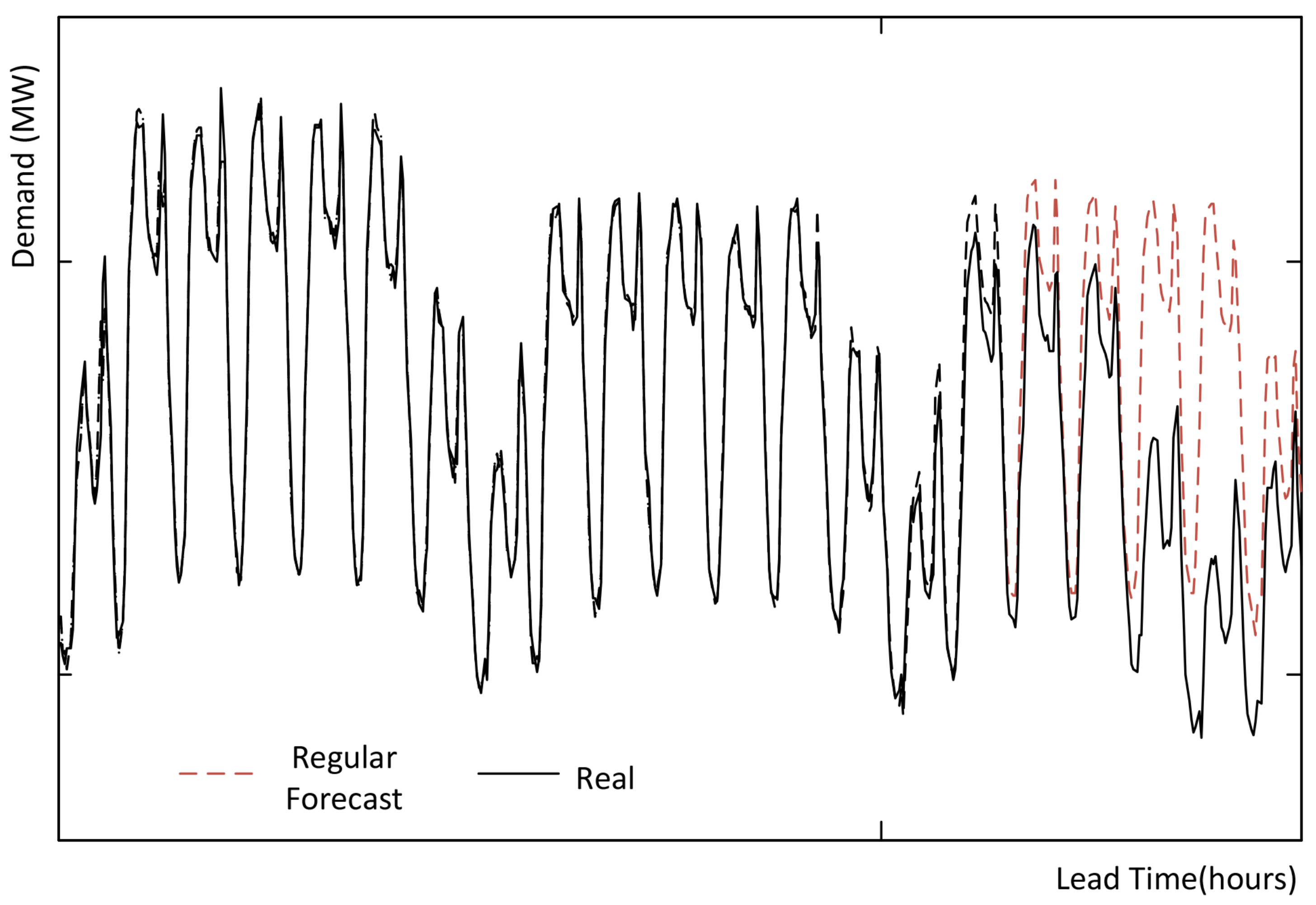
Figure 1 shows the electricity demand in Spain and the forecast during the Easter period. The regular Holt–Winters model tries to reproduce the behaviour of the time series and predicts the values shown by the dashed line. However, the demand on these days is lower due to the reduction of activity, and the real values—indicated by the solid line—deviate from the predicted values by a considerable amount. Thus, the time series shows an anomalous demand that the time series model is not able to reproduce when it is different from the pattern observed previously. This is due to the special event.

The rest of the paper is organised as follows: Section 2 reports relevant works related to predictions for special events. Section 3 introduces the methodology proposed in this paper and describes the model proposed for the study case. The most relevant results obtained by the methodology are discussed in Section 4. Finally, the conclusions drawn from this research work are summarised in Section 5.

2. Forecasting for Special Events

Due to the importance of the variation of the electricity demand on special days, a large number of methods have been developed to solve this issue. However, the developed works have aimed to use exogenous variables to modify the results of the prediction of a general model. Darbellay and Slama [24] separate the electricity demand of Wales into two models, one for special days and the other for the calendar days, and create different models for prediction in each of these situations. Smith [25] substitutes a holiday day for a Sunday. These methods have been used traditionally and are still used. Zhang and Wang [26] use similar techniques by developing decomposition–ensemble models.

Another way to tackle the problem is through the utilisation of hybrid models of regression with binary variables. Cancelo et al. [21] and later Moral-Carcedo and Vicens-Otero [27] explain how REE’s model includes the calendar effect. In their work they present one model for the midterm (as many as 10 days) and 24 models, one for each hour. The procedure carried out to obtain those models consists in separating the regular component of the electricity demand, named basic consumption, from the other two components associated with the calendar effect and weather conditions. From this itemisation, the effects produced by the calendar effect are included using binary variables correlated with a polynomial of lags. This polynomial includes a set of parameters to be determined, which depend on the class of holiday, day, hour, and position in the week, amongst others. This leads to the need to use an extremely large number of variables. Other methods commonly used consist of ARIMA models with interventions. Pardo et al. [28] developed a new model based on interventions for Spanish demand. Elanim and Fusushige [29] developed a SARIMAX model for Japanese electricity generation forecasting using data obtained from Tokyo Electric Power Corporation. The SARIMAX model included exogenous variables called effects, which are split into two groups: main and cross effects. Holidays and weather variables are included as dummy variables. Çevik and Çunkas [30] used two fuzzy logic models, the first with the previous year’s information and the second with a scaling process to produce forecasts. Kulkarni et al. [31] used spiking neural networks in which every holiday was modelled with a neuron. Erişen [32] presented a Holt–Winters model including a modification to improve forecasts for holidays.

In the last years, other points of view have been proposed that attempt to integrate these irregularities as part of their own models. Arora and Taylor [33] presented a triple seasonal Holt–Winters model based on rules and the concept of similar days. In particular, four rules are intended to change the recursivity length of the intra-annual seasonality to one similar to previous days. However, this method does not use the information provided by the method’s own irregularities. The same method was also applied to ARIMA models in [34].

In addition, Bermúdez [35] used covariates in the exponential smoothing methods for Spanish electricity demand forecasting. A new quantitative covariate reflecting the type of special day was defined within the model. Thus, a weight depending on the category was assigned. Furthermore, another variable related to the period of Easter was also added. Göb et al. [36] also used covariates in state space models applied to electricity demand in Italy. Another different technique was developed by Martínez et al. [20], which proposed a forecasting algorithm based on sequences of patterns that make it possible to distinguish the different kinds of days as a step prior to the prediction of the Spanish electricity demand.

This work presents a new point of view in which irregularities are included within the multiple seasonal Holt–Winters model as new seasonalities. The special events occur on specific days of the year, but as a general standard they develop a pattern that repeats over and over in the course of its appearance. However, this circumstance can only appear in a certain moment of the time series, and therefore it should be discrete. Due to this fact, Holt–Winters models with discrete-interval moving seasonality are developed and proposed in this work to deal with the forecasting on special days.

3. Materials and Methods

3.1. Holt–Winters Models with Discrete Interval Moving Seasonalities

The multiple seasonal Holt–Winters models have their roots in the proposal made by Taylor in 2003. He presented a nested relation between intraday and intraweek seasonalities. Later in 2010, Taylor [11] presented a new model that included the intra-annual seasonality. Finally, García-Díaz and Trull [37] proposed a generalisation of this methodology, named nHWT, to deal with any number of seasonalities.

Following [37], a model with an additive trend and multiplicative seasonality would be expressed as Equations (1)–(4).

$$\begin{array}{ccc}\hfill L_t& =& \alpha \left(\frac{X_t}{{\prod }_{i=1}^{n_s}{I}_{t-s_i}^{\left(i\right)}}\right)+(1-\alpha )(L_{t-1}+T_{t-1})\hfill \end{array}$$

(1)

$$\begin{array}{ccc}\hfill T_t& =& \gamma (L_t-L_{t-1})+(1-\gamma )T_{t-1}\hfill \end{array}$$

(2)

$$\begin{array}{ccc}\hfill I_t^{\left(i\right)}& =& {\delta }^{\left(i\right)}\left(\frac{X_t}{L_t{\prod }_{j=1,j\ne i}^{n_s}{I}_{t-s_j}^{\left(j\right)}}\right)+(1-{\delta }^{\left(i\right)})I_{t-s_i}^{\left(i\right)}i=1,\cdots ,n_s\hfill \end{array}$$

(3)

$$\begin{array}{ccc}\hfill {\widehat{X}}_{t+k}& =& (L_t+k{T}_t)\prod _{i=1}^{n_s}{I}_{t-s_i+k}^{\left(i\right)}+{\phi }_{AR}^k{ϵ}_t\hfill \end{array}$$

(4)

where $L_t$ and $T_t$ are the equations for the level and additive trend, with smoothing parameters $\alpha$ and $\gamma$. $I_t^{\left(i\right)}$ are the seasonal indices of length $s_i$, with smoothing parameters ${\delta }^{\left(i\right)}$. There are as many equations as seasonal patterns allocated in the time series, $n_s$. $X_t$ is the observed data. Finally, ${\widehat{X}}_{t+k}$ is the equation to forecast k time instants ahead. It collects the information contained in the model and makes predictions. To include the adjustment for the first-order autocorrelation error, ${\phi }_{AR}$ is added, and ${ϵ}_t$ is white noise. In case this adjustment is avoided: ${\phi }_{AR}=0$.

Following [37], the following system of nomenclature simplified with three letters is used. The first indicates the type of trend, the second the type of seasonality, and the third whether the model has been adjusted with the first-order autocorrelation error. Numbers indicating the length of every seasonal period considered are additionally specified as subscripts. As an example, the model $AM{C}_{24,168}$ denotes the model described in Equations (1)–(4) with two seasonalities: intraday and intraweek, with lengths of 24 and 168 h, respectively.

The relation between seasonalities is governed by a fixed ratio during the whole-time range of the series (for instance, a week is 7 days). Moreover, both seasonalities should establish a fixed beginning (Monday at 0:00).

Nevertheless, Easter has a different behaviour. The holiday period is established according to a religious calendar and starts on a different date every year. In that period, the electricity demand varies substantially compared with a regular period. Holt–Winters models cannot adapt to this irregularity themselves. A similar case applies to Christmas.

The new seasonal pattern $D_{t_h^{*}}$ is defined only in $t_h^{*}$, which is a discretization of time that represents the time instants of the time series $X_t$ where the special event provokes one change of the demand. This time is not necessarily coincident with the holidays but coincides with the time of influence. It has a fixed period length $s_h$. As the special event can take place on different dates, the recursivity of the pattern should vary and adapt at every new appearance. So, the recursivity is then defined as $s_h^{*}$ regardless of the length of the seasonal pattern. This new seasonality is a discrete-interval moving seasonality (DIMS), with $n_{DIMS}$ being the number of DIMS considered. Thus DIMS is defined as follows:

$$D_{t_h^{*}}^{\left(h\right)}={\delta }_D^{\left(h\right)}\left(\frac{X_t}{L_t{\prod }_{i=1}^{n_s}{I}_{t-s_i}^{\left(i\right)}{\prod }_{m=1,m\ne h}^{n_{DIMS}}{D}_{t_m^{*}-s_m^{*}}^{\left(m\right)}}\right)+(1-{\delta }_D^{\left(h\right)})D_{t_h^{*}-s_h^{*}}^{\left(h\right)}h=1,\dots ,n_{DIMS}$$

(5)

where $D_{t_h^{*}}^{\left(h\right)}$ are the new seasonal equations defined for DIMS with a period length of $s_h$, with smoothing parameter ${\delta }_D^{\left(h\right)}$. As explained, $D_{t_h^{*}}^{\left(h\right)}$ is defined only in $t_h^{*}$, with a recurrence of $t_h^{*}-s_h^{*}$.

This new seasonal pattern is integrated in the complete model according to the methods established for the seasonality, as expressed by Equations (6)–(10).

$$\begin{array}{ccc}\hfill L_t& =& \alpha \left(\frac{X_t}{{\prod }_{i=1}^{n_s}{I}_{t-s_i}^{\left(i\right)}{\prod }_{h=1}^{n_{DIMS}}{D}_{t_h^{*}-s_h^{*}}^{\left(h\right)}}\right)+(1-\alpha )(L_{t-1}+T_{t-1})\hfill \end{array}$$

(6)

$$\begin{array}{ccc}\hfill T_t& =& \gamma (L_t-L_{t-1})+(1-\gamma )T_{t-1}\hfill \end{array}$$

(7)

$$\begin{array}{ccc}\hfill I_t^{\left(i\right)}& =& {\delta }^{\left(i\right)}\left(\frac{X_t}{L_t{\prod }_{j=1,j\ne i}^{n_s}{I}_{t-s_j}^{\left(j\right)}{\prod }_{h=1}^{n_{DIMS}}{D}_{t_h^{*}-s_h^{*}}^{\left(h\right)}}\right)+(1-{\delta }^{\left(i\right)})I_{t-s_i}^{\left(i\right)}\hfill \end{array}$$

(8)

$$\begin{array}{ccc}\hfill D_{t_h^{*}}^{\left(h\right)}& =& {\delta }_D^{\left(h\right)}\left(\frac{X_t}{L_t{\prod }_{i=1}^{n_s}{I}_{t-s_i}^{\left(i\right)}{\prod }_{m=1,m\ne h}^{n_{DIMS}}{D}_{t_m^{*}-s_m^{*}}^{\left(m\right)}}\right)+(1-{\delta }_D^{\left(h\right)})D_{t_h^{*}-s_h^{*}}^{\left(h\right)}\hfill \end{array}$$

(9)

$$\begin{array}{ccc}\hfill {\widehat{X}}_{t+k}& =& (L_t+k{T}_t)\prod _{i=1}^{n_s}{I}_{t-s_i+k}^{\left(i\right)}\prod _{h=1}^{n_{DIMS}}{D}_{t_h^{*}-s_h^{*}+k}^{\left(h\right)}+{\phi }_{AR}^k{ϵ}_t\hfill \end{array}$$

(10)

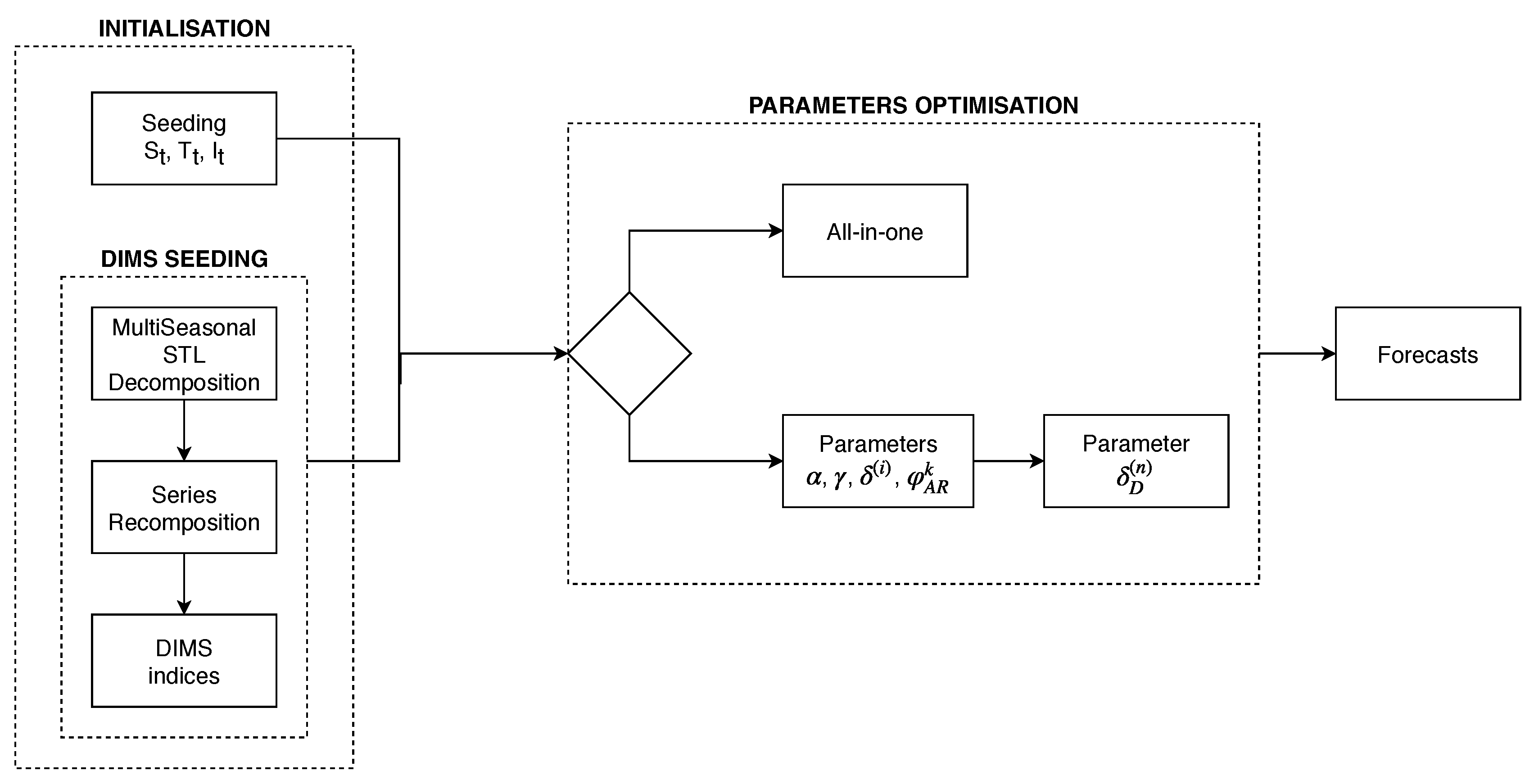
The model exhibited is a method that considers multiplicative seasonality. The methods that consider additive seasonality, such as $AA{C}_{24,168}$, which include the additive trend and seasonalities, would be similar to the one shown, but with the DIMS multiplicative factors and seasonalities exchanged for addends. Working with DIMS needs a different procedure to the usual one since the initial values of the DIMS are calculated separately. However, when working with a seasonality, this seasonality needs to have appeared at least once before being able to be used to make forecasts. Figure 2 shows the workflow of the procedure, which is detailed hereafter.

3.1.1. Obtaining Seeds of the Model

The first step to get seeds for the model consists in determining the initial values of the regular model. For this case, multiple seasonal techniques have been used. The level is determined as the moving average for the two first cycles of greater length. The trend is obtained from the slope between the two first cycles of longer length and modified by the contribution of the cycles of shorter length. Finally, the seasonality is determined as the ratio between the values of the series for the first cycles over the moving average, with this value being distributed between the different seasonalities next.

In order to determine the seeds of DIMS, firstly a decomposition of the time series is carried out using an appropriate technique. In this work, decomposition of the trend and multiple seasonality based on Loess (STL) is used [38]. The series is thus decomposed as in Equation (11).

$$X_t=T_t+\sum S_t^{\left(s_i\right)}+U_t$$

(11)

where $T_t$ represents the trend and $S_t^{\left(s_i\right)}$ are the seasonal indices for each of the considered seasonal patterns in the model. $U_t$ stands for the residuals, from which the information for DIMS will be obtained.

In the second step, the series is reassembled again using Equation (12). Here it is fundamental to understand clearly that the remainder should not be included in the rebuilt series, since the information that needs to be analysed is found in it.

$$R_t=T_t+\sum S_t^{\left(s_i\right)}$$

(12)

where $R_t$ is the rebuilt series without including the remainder $U_t$. Finally, it is necessary to get values from the indices. For this purpose, it is first necessary to get the weights for the time series over the reassembled time series.

Table 1. Estimate of the weights of the values of the series on the rebuilt time series. In the columns each appearance of the discrete-interval moving seasonality (DIMS) is shown, and in the rows every time instant within the discrete seasonality.

	1	2	3	…	n
1	$\frac{X_{p_1}}{R_{p_1}}$	$\frac{X_{p_2}}{R_{p_2}}$	$\frac{X_{p_3}}{R_{p_3}}$	…	$\frac{X_{p_n}}{R_{p_n}}$
2	$\frac{X_{p_1+1}}{R_{p_1+1}}$	$\frac{X_{p_2+1}}{R_{p_2+1}}$	$\frac{X_{p_3+1}}{R_{p_3+1}}$	…	$\frac{X_{p_n+1}}{R_{p_n+1}}$
…	…	…	…		…
$s_h$	$\frac{X_{p_1+s_h-1}}{R_{p_1+s_h-1}}$	$\frac{X_{p_2+s_h-1}}{R_{p_2+s_h-1}}$	$\frac{X_{p_3+s_h-1}}{R_{p_3+s_h-1}}$	…	$\frac{X_{p_n+s_h-1}}{R_{p_n+s_h-1}}$

shows how to calculate the values of the weights. This table is organised so that each column represents every one of the appearances of the discrete seasonality. Each of the data observed in each seasonality is arranged in the rows. The necessary quantity of data will be determined for $s_h$, which is the length of the DIMS period. The values of $p_i$ are the time positions within the time series, and n stands for the number of occurrences of the event within the time series.

Finally, the seasonal indices are obtained as the average of the values indicated previously, as shown in Equation (13).

$$D_t^{\left(h\right)}=\frac{1}{n}\sum _{j=1}^n\frac{X_{p_j+t-1}}{R_{p_j+t-1}},t=1,\dots ,s_h$$

(13)

It is important to distinguish $s_h$ and $s_h^{*}$. The former refers to the length of the seasonal discrete pattern, while the latter refers to the recurrent distance to find the previous event.

3.1.2. Parameter Optimisation and Forecast

The role of the parameters is fundamental in the Holt–Winters models. A search for parameters is performed, to determine their ability to adapt the model, as far as possible, to the observed data. For this purpose, methods of minimisation of the forecasting error for a training set are used. There are many measures that can be used to determine the level of the error in the prediction and that are useful for the process of minimisation. In this work, the root mean square error (RMSE) is used Equation (14).

$$\mathrm{RMSE}=\sqrt{\frac{1}{N}\sum {({\widehat{X}}_t-X_t)}^2}$$

(14)

The minimisation of the RMSE is a nonlinear problem and the search space is defined by the smoothing parameters as shown in Equation (15).

$$\begin{array}{cc}\underset{(\alpha ,\gamma ,{\delta }^{\left(i\right)},{\phi }_{AR})\in \Omega }{\mathrm{minimize}}\hfill & \mathrm{RMSE}\hfill \end{array}$$

(15)

Note that the feasibility region $\Omega$ is bounded between 0 and 1.

As can be appreciated from Figure 2, two options are proposed in order to minimise the RMSE:

• The first consists in determining all parameters simultaneously. Chatfield [39] studied the optimisation of the parameters separately and jointly. He concluded that the best solution is to accomplish the joint optimisation of the parameters.
• The second consists in accomplishing an optimisation of the regular model and subsequently optimising the parameters of the DIMS. Although this contradicts the previous point of view, no differences in precision are found, but there are differences in optimisation time.

Once the model has been adjusted, the forecast is carried out for a test set. In order to measure the accuracy of the prediction, the RMSE can be used again. But in this case, the predictions are commonly compared using the Mean Absolute Percentage Error (MAPE), as defined in Equation (16).

$$\mathrm{MAPE}(\%)=100·\frac{1}{N}\sum \left|\frac{{\widehat{X}}_t-X_t}{X_t}\right|$$

(16)

This work analyses very short-term forecasts: usually 24 h ahead, but also 168 h ahead. The forecasts are obtained from the last observed data and are compared with the real values in order to check the accuracy of the proposed model.

3.2. A Case Study: Easter

The objective of this section is to show the prediction models for a study case, in particular, the forecasting of electricity demand when modelling the Easter effect by means of the DIMS.

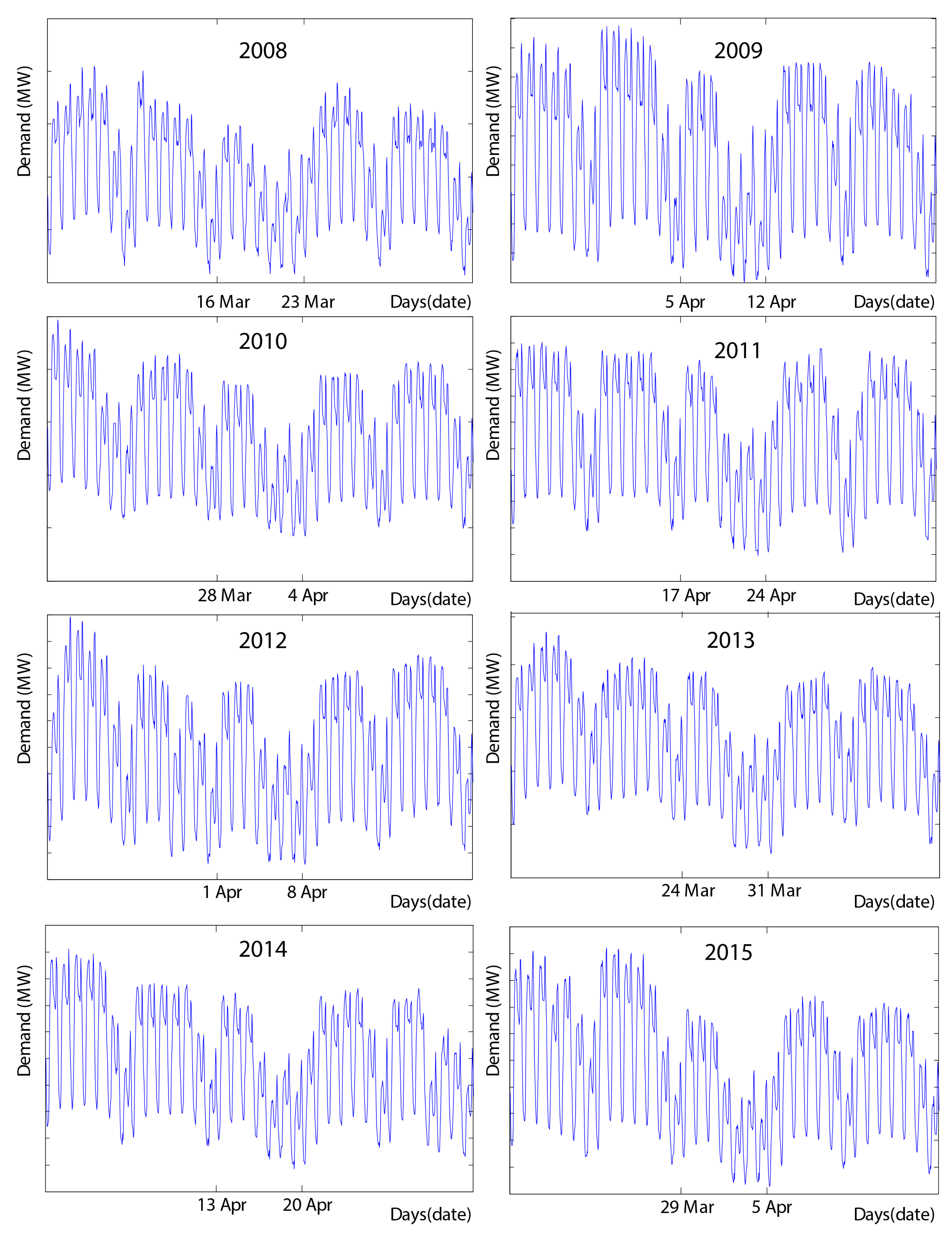
For the study, it is important to observe Figure 3, which presents the hourly electricity demand in Spain in the weeks around Easter for the years from 2008 to 2015. It can be appreciated that the effect of Easter provokes a decrease in electricity consumption during a fixed period and that this decrease remains from Holy Thursday to the day after Easter Sunday. This is repeated in all of the years, although Easter happens in different periods of the year. The date of Easter is variable, since it depends on the first full moon after the spring equinox.

It can be seen that all days of the week are affected by the holidays. This is due to the fact that the official Easter in Spain begins on Good Friday and ends with Resurrection Sunday. However, in many regions, Thursday, Monday, or both are also holidays. This provokes a decrease in activity.

In this work, forecasts for Easter in 2014 and 2015 are obtained using the information provided by the time series and considering the Easter periods from 2008. For that purpose, two Holt–Winters models with DIMS and two seasonal patterns (24 and 168 h) have been used. The first is a model with multiplicative seasonality named $AM{C}_{24,168,Easter}$. The second one has additive seasonality and is named $AA{C}_{24,168,Easter}$. The $AM{C}_{24,168,Easter}$ model is shown in Equations (17)–(22), where ${\delta }_D^{\left(Easter\right)}$ stands for the smoothing parameter used in the Easter DIMS.

$$\begin{array}{ccc}\hfill L_t& =& \alpha \left(\frac{X_t}{I_{t-24}^{\left(24\right)}{I}_{t-168}^{\left(168\right)}{D}_{t_{Easter}^{*}-s_{Easter}^{*}}^{\left(Easter\right)}}\right)+(1-\alpha )(L_{t-1}+T_{t-1})\hfill \end{array}$$

(17)

$$\begin{array}{ccc}\hfill T_t& =& \gamma (L_t-L_{t-1})+(1-\gamma )T_{t-1}\hfill \end{array}$$

(18)

$$\begin{array}{ccc}\hfill I_t^{\left(24\right)}& =& {\delta }^{\left(24\right)}\left(\frac{X_t}{L_t{I}_{t-168}^{\left(168\right)}{D}_{t_{Easter}^{*}-s_{Easter}^{*}}^{\left(Easter\right)}}\right)+(1-{\delta }^{\left(24\right)})I_{t-24}^{\left(24\right)}\hfill \end{array}$$

(19)

$$\begin{array}{ccc}\hfill I_t^{\left(168\right)}& =& {\delta }^{\left(168\right)}\left(\frac{X_t}{L_t{I}_{t-24}^{\left(24\right)}{D}_{t_{Easter}^{*}-s_{Easter}^{*}}^{\left(Easter\right)}}\right)+(1-{\delta }^{\left(168\right)})I_{t-168}^{\left(168\right)}\hfill \end{array}$$

(20)

$$\begin{array}{ccc}\hfill D_{t_{Easter}^{*}}^{\left(Easter\right)}& =& {\delta }_D^{\left(Easter\right)}\left(\frac{X_t}{L_t{I}_{t-24}^{\left(24\right)}{I}_{t-168}^{\left(168\right)}}\right)+(1-{\delta }_D^{\left(Easter\right)})D_{t_{Easter}^{*}-s_{Easter}^{*}}^{\left(Easter\right)}\hfill \end{array}$$

(21)

$$\begin{array}{ccc}\hfill {\widehat{X}}_{t+k}& =& (L_t+k{T}_t)I_{t-24+k}^{\left(24\right)}{I}_{t-168+k}^{\left(168\right)}{D}_{t_{Easter}^{*}-s_{Easter}^{*}+k}^{\left(Easter\right)}+{\phi }_{AR}^k{ϵ}_t\hfill \end{array}$$

(22)

Next, it is necessary to determine the values of $t_{Easter}^{*}$ and $s_{Easter}^{*}$ in order to define the aforementioned models completely.

Due to the fact that the Easter holidays are not the same across the whole of Spain and that they also have a small annual variation in some regions, it is difficult to establish an exact period for the Easter prediction. As a starting point, the discrete period between Holy Thursday and Easter Monday has been analysed, since it seems to be where a greater influence is clearly seen. The Easter period for each year is illustrated in

Table 2. General Easter period in Spain.

Year	Palm Sunday	Resurrection	${\mathit{t}}_{\mathit{Easter}}^{*}$		${\mathit{s}}_{\mathit{Easter}}^{*}$
		Sunday	Begin	End
2008	16 March	23 March	1897	2017	—
2009	5 April	12 April	11,237	11,257	9220
2010	28 March	4 April	19,705	19,825	8448
2011	17 April	24 April	28,945	29,065	9120
2012	1 April	8 April	37,345	37,465	8280
2013	24 March	31 March	45,913	46,033	8448
2014	13 April	20 April	55,153	55,273	9120
2015	29 March	5 April	63,553	63,673	8280

. It starts with Palm Sunday and ends with Resurrection Sunday. This table shows when these special days occur. Not all regions in Spain apply the same Easter period for holidays, but all of them include, at least, Holy Thursday and Friday. In columns 4 and 5, the interval in which the discrete seasonality is defined for each year is shown. The ‘Beginning’ column starts with Holy Thursday and shows the position of the DIMS in the hourly time series. In the last column, the value of recursivity, in hours, is shown for each event. As an example, Easter starts on Holy Thursday on 28 March 2013 (position 45,913 in the time series) and finishes on Easter Sunday (position 46,033), which represents a length $s_h$ of 120 h. Therefore, $D_{t_{Easter}^{*}}^{\left(Easter\right)}$ in 2013 only is defined between these two values. In order to determine the recursivity, the previous year has to be analysed. The Easter of the year 2012 ended up in 8 April (position 37,465 in the time series), and therefore the recursivity was 8448 h in that year.

4. Results and Discussion

With the aim of validating the new proposal experimentally, the Spanish electricity demand data from REE have been used. In particular, the time series is the hourly electricity demand aggregated for the Iberian Peninsula from January 2008 to July 2015. As Easter is a source of important irregularity, the two DIMS models specified in Section 4 ($AA{C}_{24,168,Easter}$ and $AM{C}_{24,168,Easter}$) have been applied to obtain predictions for the days of Easter in 2014 and 2015.

4.1. Analysis of Results

In order to obtain the parameters of the model, minimisation of the RMSE is carried out using data from 1 January 2008 until the day before Holy Thursday of 2014. Both methods, that is, the all-in-one method (hereafter M1) and the two-step method (M2), have been used but the differences amongst the parameters and the results are not significant. The parameters obtained using the two-step optimisation method are shown in

Table 3. Smoothing parameters for the models used to predict the days of Easter in 2014 and 2015.

Model	$\mathit{\alpha }$	$\mathit{\gamma }$	${\mathit{\delta }}^{\left(24\right)}$	${\mathit{\delta }}^{\left(168\right)}$	${\mathit{\delta }}^{\left(\mathit{Easter}\right)}$	${\mathit{\phi }}_{\mathit{AR}}$
$AM{C}_{24,168,Easter}$	0.0502	0.0001	0.3080	0.0614	0.0627	0.9178
$AA{C}_{24,168,Easter}$	0.0001	0.0071	0.2981	0.1127	0.1167	0.9658

. The data used to fit the model went up to the day before Holy Thursday of 2014.

From the point of view of demand, it is not really clear whether the discrete beginning of the period should begin on Holy Thursday or on Monday, since, as mentioned above, the holidays are different in each region. In a similar way, the Monday after Easter is not always a holiday, even in the same region. This point led us to analyse several options and to check which one of them offered the best results. On one hand, the day on which Easter begins is considered, as well as the period included in the analysis and the method of optimising the parameters of the model. Therefore, several starting positions and lengths were tested with the aim of finding out the best DIMS definitions for the Easter period. The setting used for the analysis are summarised in

Table 4. Periods analysis setting.

Period	Starting at	Length
0	Regular Model, no DIMS included
1	Monday after Palm Sunday	192 h
2	Holy Thursday	120 h

. It can be seen that three cases have been analysed. Case 0 represents the regular nHWT model, without including any DIMS. Case 1 is associated with period 1, which includes the DIMS starting on Monday after Palm Sunday, with a length of 192 h (up to Monday after Resurrection Sunday). In Case 2, corresponding to period 2, the DIMS starts on Holy Thursday and has a length of 120 h. All periods started at 00:00 hours.

Table 5. Mean Absolute Percentage Error (MAPE) for $AM{C}_{24,168}$, $AM{C}_{24,168,Easter}$, $AA{C}_{24,168}$, and $AA{C}_{24,168,Easter}$ for different periods and optimisation methods.

MODEL		${\mathit{AMC}}_{24,168}$	${\mathit{AMC}}_{24,168,\mathit{Easter}}$			${\mathit{AAC}}_{24,168}$	${\mathit{AAC}}_{24,168,\mathit{Easter}}$
VARIANT		CASE 0	CASE 1	CASE 2		CASE 0	CASE 1	CASE 2
				M2	M1			M2	M1
Thursday	17/04/2014	13.12	3.05	2.73	2.79	12.25	6.42	5.90	9.18
Friday	18/04/2014	11.38	1.74	2.41	3.06	14.22	1.79	2.39	2.14
Saturday	19/04/2014	10.97	1.68	1.44	1.58	11.34	1.40	1.28	1.09
Sunday	20/04/2014	3.25	1.65	1.88	4.04	5.85	4.33	4.67	4.79
Monday	21/04/2014	4.94	6.25	3.57	7.02	5.80	4.87	5.06	5.87
Thursday	02/04/2015	11.35	2.90	2.79	3.07	12.02	5.47	4.81	8.80
Friday	03/04/2015	10.66	3.44	1.55	2.62	12.82	0.97	1.13	2.44
Saturday	04/04/2015	10.51	1.10	2.58	2.04	10.32	2.64	2.45	2.28
Sunday	05/04/2015	3.60	2.56	1.53	2.47	4.86	3.11	3.44	2.88
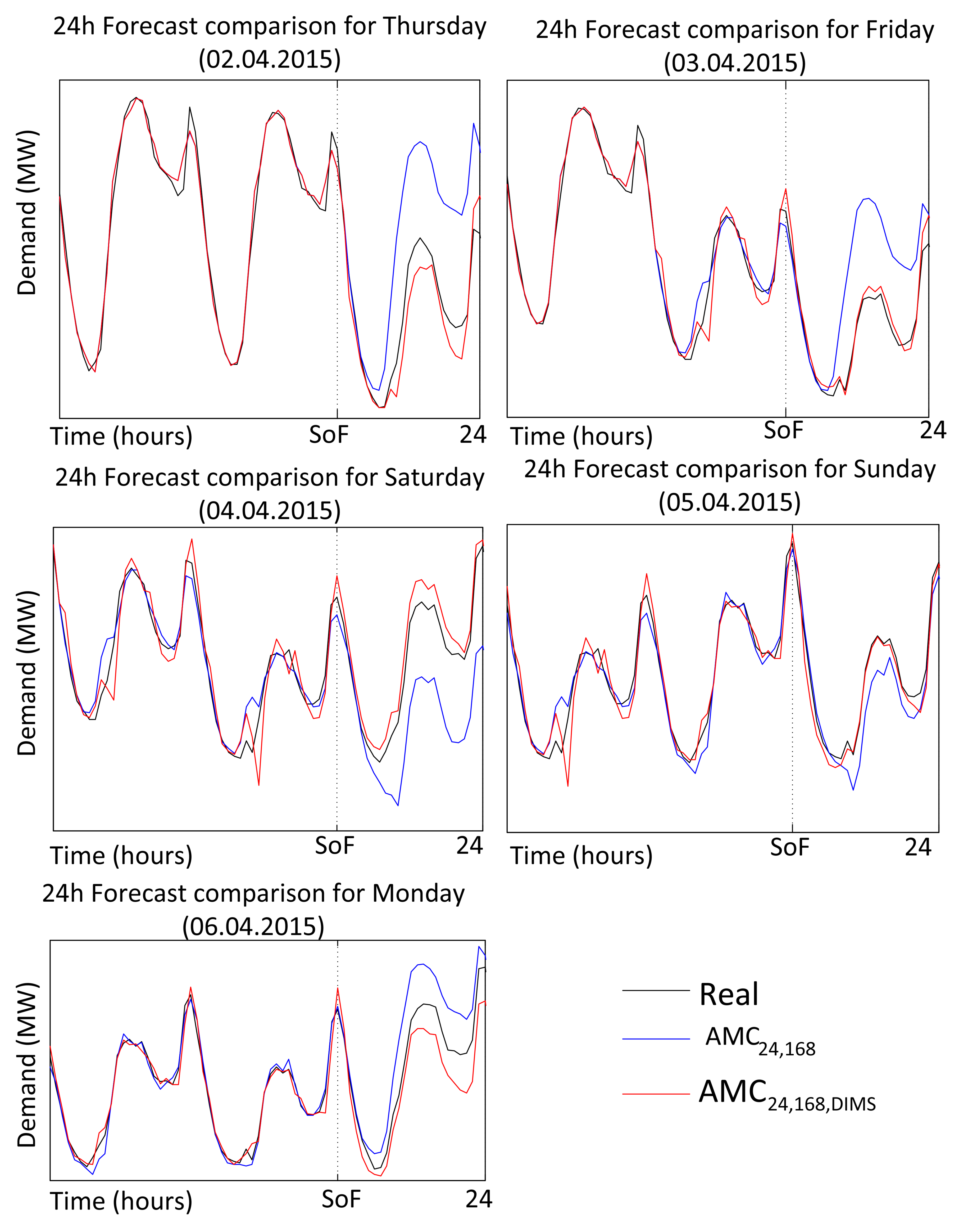
Monday	06/04/2015	5.91	1.51	3.93	4.69	7.40	2.84	3.04	2.96

summarises the results obtained when predicting the Easter demand for the years 2014 and 2015. For case 0, it can be seen that the model cannot operate with Easter and therefore the MAPE rises, reaching values of up to 13%, in comparison to the forecast on a typical day, when it hovers around 2% [37]. Models that include DIMS provide MAPE under 5%. This provides evidence that the inclusion of the DIMS has improved the results substantially. However, the comparison between cases 1 and 2 does not yield big differences, and therefore case 2 has been selected in order to show the results obtained by the optimisation methods M1 and M2, since it includes a shorter period of seasonality. In relation to the optimisation method, the variation of the MAPE is not fundamental, being the two-step method much faster. The ranges of precision obtained have MAPE values that hover around 1.5% to 3%, very near to the typical values for nHWT on a workday. In order to verify this situation, Figure 4 shows the forecast for the next 24 h for each day of Easter in 2015, with a regular nHWT model in comparison to the new $AM{C}_{24,168,Easter}$ including DIMS. It can be appreciated that the new methodology obtains forecasts nearer to the real data.

4.2. Comparison

An analysis in order to benchmark the proposed method against other methods commonly used in the literature have been conducted. Three alternative methods have been considered: Artificial Neural Network (ANN), the TBATS model, and the TBATS model including exogenous variables. ANN is a general-purpose method and TBATS are models that include moving seasonal effects to predict special days.

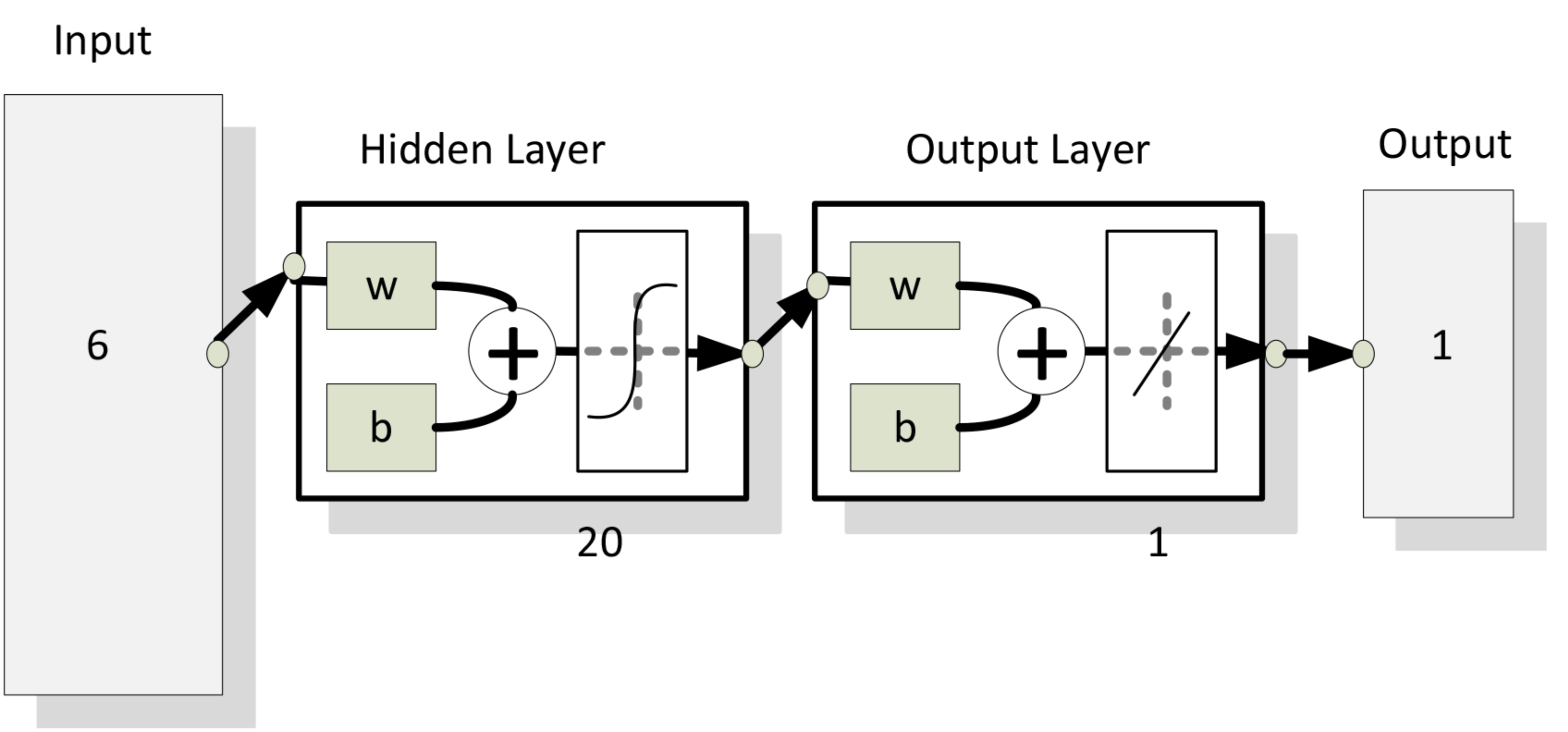
ANN is a computational method that tries to simulate the behaviour of the human brain. It comprises interconnected neurons that are organised in layers and can be trained. This training assigns weights to neurons according to a determined pattern. In the last years, the use of neural network methods is increasing, according to new studies about the human brain, and offer new possibilities. In short-term load forecasting, the ANN learns from past data and can provide forecasts of future demands. In many works the ANN is not used as a standalone method but as a part of other models. He et al. [40] provides a good explanation of the usage of ANN. Our study uses a neural network regression model, as shown in Figure 5. It has a hidden layer with 20 neurons, and as inputs, in addition to load forecasting, the day of the week, a variable indicating the special day events, and some other variables to help deal with seasonalities have been included.

The Exponential Smoothing State Space Model with Box-Cox Transformation, ARMA Errors, Trend and Seasonal Components (TBATS) evolved from state space models. De Livera [41] described how the addition of the Box-Cox transformation dealing with the non-linearities in the time series and including an ARMA process in the residuals to include possible autocorrelations improved the results obtained with state space models. These are BATS models. Latterly, De Livera et al. [12], developed TBATS by developing a Fourier series to deal with seasonalities in the model, which reduced the number of parameters to be used. They applied a methodology to include special days in the model. In this analysis, the same procedure to Spanish electricity demand, with and without regressors, has been applied.

Figure 6 shows the MAPE obtained by all methods using the same dataset for all of the Easter days from Thursday to Monday. The names used in the graph correspond to the method used to obtain the forecasts. The name TBATS JASA refers to TBATS with regressors; this name is used due to the fact that the method explained in [12] has been applied. It is clear that TBATS using regressors outperforms TBATS, but $AM{C}_{24,168,DIMS}$ outperforms the rest. The ANN obtained an average MAPE of 3.08%, while $AM{C}_{24,168,DIMS}$ obtained a value of 2.5%.

5. Conclusions

After analysing the problems of the existence of irregularities in the time series of the electricity demand in Spain, the possibility of using Holt–Winters models with discrete-interval seasonalities has been analysed. The DIMS have been described as a logical solution and are in-built within the regular Holt–Winters models. Then, the models have been applied to predict the demand for the Easter holidays, allowing the efficacy of the DIMS to be checked. The different possibilities for forecasting the demand for Easter using the DIMS have been analysed, and it has been concluded that the best choice is to use one DIMS from Holy Thursday to the Monday after Easter. The obtained results shown a MAPE improvement of around 11% from the regular models to below 3%. The utilisation of discrete seasonalities makes it possible to apply singular patterns at punctual moments of the time series. These patterns are not necessarily related to a fixed sequence and they can be arranged in different moments of the time series. Furthermore, the patterns can be repeated as often as necessary in a period of time and in different periods, but does not necessarily have to be repeated. It is only necessary for it to have appeared prior to the forecast. Regarding the smoothing parameters, the inclusion of this new discrete seasonality helped the intraweek seasonality to deal with the irregularities that are associated with it. As a result, their smoothing parameters have lower values that are closer to 0. A comparison among different methods is also conducted. The results show that the use of DIMS improves the results and that this method outperforms the other methods.

Future works should aim to exploit the characteristic of being flexible in respect of the position in time. Moreover, the model could permit the coexistence of a large number of discrete seasonalities when more than one discrete seasonality is able to coexist with another seasonality. This can allow DIMS to be used in a general model and thus to model the calendar effect.

References

- Garrués-Irurzun, J.; López-García, S. Red Eléctrica de España S.A.: Instrument of regulation and liberalization of the Spanish electricity market (1944–2004). Renew. Sustain. Energy Rev. 2009, 13, 2061–2069. [Google Scholar] [CrossRef]
- Domínguez, E.F.; Bernat, J.X. Restructuring and generation of electrical energy in the Iberian Peninsula. Energy Policy 2007, 35, 5117–5129. [Google Scholar] [CrossRef]
- Hobbs, B.F. Analysis of the value for unit commitment of improved load forecasts. IEEE Trans. Power Syst. 1999, 14, 1342–1348. [Google Scholar] [CrossRef]
- Hirth, L.; Ziegenhagen, I. Balancing power and variable renewables: Three links. Renew. Sustain. Energy Rev. 2015, 50, 1035–1051. [Google Scholar] [CrossRef] [Green Version]
- Roldán-Fernández, J.; Gómez-Quiles, C.; Merre, A.; Burgos-Payán, M.; Riquelme-Santos, J.M. Cross-border energy exchange and renewable premiums: The case of the Iberian system. Energies 2018, 11, 3277. [Google Scholar] [CrossRef]
- Weron, R. Modeling and Forecasting Electricity Loads and Prices: A Statistical Approach; John Wiley & Sons: Hoboken, NJ, USA, 2007; Volume 403. [Google Scholar]
- Contreras, J.; Espinola, R.; Nogales, F.J.; Conejo, A.J. ARIMA models to predict next-day electricity prices. IEEE Trans. Power Syst. 2003, 18, 1014–1020. [Google Scholar] [CrossRef] [Green Version]
- Juberias, G.; Yunta, R.; Garcia Moreno, J.; Mendivil, C. A new ARIMA model for hourly load forecasting. In Proceedings of the 1999 IEEE Transmission and Distribution Conference, New Orleans, LA, USA, 11–16 April 1999; pp. 314–319. [Google Scholar] [CrossRef]
- Bianco, V.; Manca, O.; Nardini, S. Electricity consumption forecasting in Italy using linear regression models. Energy 2009, 34, 1413–1421. [Google Scholar] [CrossRef]
- Taylor, J.W. Short-term electricity demand forecasting using double seasonal exponential smoothing. J. Oper. Res. Soc. 2003, 54, 799–805. [Google Scholar] [CrossRef] [Green Version]
- Taylor, J.W. Triple seasonal methods for short-term electricity demand forecasting. Eur. J. Oper. Res. 2010, 204, 139–152. [Google Scholar] [CrossRef] [Green Version]
- De Livera, A.M.; Hyndman, R.J.; Snyder, R.D. Forecasting time series with complex seasonal patterns using exponential smoothing. J. Am. Stat. Assoc. 2011, 106, 1513–1527. [Google Scholar] [CrossRef]
- Hyndman, R.; Koehler, A.; Ord, J.; Snyder, R. Forecasting with Exponential Smoothing: The State Space Approach; Springer: Berlin/Heidelberg, Germany, 2008. [Google Scholar]
- Ko, C.; Lee, C. Short-term load forecasting using SVR (support vector regression)-based radial basis function neural network with dual extended Kalman filter. Energy 2013, 49, 413–422. [Google Scholar] [CrossRef]
- Rana, M.; Koprinska, I. Forecasting electricity load with advanced wavelet neural networks. Neurocomputing 2016, 182. [Google Scholar] [CrossRef]
- Baliyan, A.; Gaurav, K.; Kumar Mishra, S. A review of short term load forecasting using artificial neural network models. Procedia Comput. Sci. 2015, 48, 121–125. [Google Scholar] [CrossRef]
- Yang, Z.; Ce, L.; Lian, L. Electricity price forecasting by a hybrid model, combining wavelet transform, ARMA and kernel-based extreme learning machine methods. Appl. Energy 2017, 190, 291–305. [Google Scholar] [CrossRef]
- Ghadimi, N.; Akbarimajd, A.; Shayeghi, H.; Abedinia, O. Two stage forecast engine with feature selection technique and improved meta-heuristic algorithm for electricity load forecasting. Energy 2018, 161, 130–142. [Google Scholar] [CrossRef]
- Troncoso, A.; Riquelme-Santos, J.M.; Riquelme, J.; Gómez-Expósito, A.; Martínez-Ramos, J.L. Time-Series Prediction: Application to the Short-Term Electric Energy Demand. Lect. Notes Comput. Sci. 2004, 3040, 577–586. [Google Scholar] [CrossRef] [Green Version]
- Martínez-Álvarez, F.; Troncoso, A.; Riquelme, J.C.; Aguilar-Ruíz, J. Energy Time Series Forecasting Based on Pattern Sequence Similarity. IEEE Trans. Knowl. Data Eng. 2011, 23, 1230–1243. [Google Scholar] [CrossRef] [Green Version]
- Cancelo, J.R.; Espasa, A.; Grafe, R. Forecasting the electricity load from one day to one week ahead for the Spanish system operator. Int. J. Forecast. 2008, 24, 588–602. [Google Scholar] [CrossRef] [Green Version]
- Cancelo, J.; Espasa, A. Modelling and Forecasting Daily Series of Electricity Demand. Investig. Econ. 1996, 20, 359–376. [Google Scholar]
- Torro, H.; Meneu, V.; Valor, E. Single Factor Stochastic Models with Seasonality Applied to Underlying Weather Derivatives Variables. J. Risk Financ. 2003, 4, 6–17. [Google Scholar] [CrossRef]
- Darbellay, G.A.; Slama, M. Forecasting the short-term demand for electricity: Do neural networks stand a better chance? Int. J. Forecast. 2000, 16, 71–83. [Google Scholar] [CrossRef]
- Smith, M. Modeling and Short-Term Forecasting of New South Wales Electricity System Load. J. Bus. Econ. Stat. 2000, 18, 465–478. [Google Scholar] [CrossRef]
- Zhang, X.; Wang, J. A novel decomposition–ensemble model for forecasting short–term load–time series with multiple seasonal patterns. Appl. Soft Comput. 2018, 65, 478–494. [Google Scholar] [CrossRef]
- Moral-Carcedo, J.; Vicéns-Otero, J. Modelling the non-linear response of Spanish electricity demand to temperature variations. Energy Econ. 2005, 27, 477–494. [Google Scholar] [CrossRef]
- Pardo, A.; Meneu, V.; Valor, E. Temperature and seasonality influences on Spanish electricity load. Energy Econ. 2002, 24, 55–70. [Google Scholar] [CrossRef]
- Elamin, N.; Fukushige, M. Modeling and forecasting hourly electricity demand by SARIMAX with interactions. Energy 2018, 165(Part B), 257–268. [Google Scholar] [CrossRef]
- Çevik, H.H.; Çunkaş, M. A Fuzzy Logic Based Short Term Load Forecast for the Holidays. Int. J. Mach. Learn. Comput. 2016, 6, 57–61. [Google Scholar] [CrossRef]
- Kulkarni, S.; Simon, S.; Sundareswaran, K. A spiking neural network (SNN) forecast engine for short-term electrical load forecasting. Appl. Soft Comput. 2013, 13, 3628–3635. [Google Scholar] [CrossRef]
- Erisen, E.; Iyigun, C.; Tanrısever, F. Short–term electricity load forecasting with special days: An analysis on parametric and non–parametric methods. Ann. Oper. Res. 2017, 1–34. [Google Scholar] [CrossRef]
- Arora, S.; Taylor, J. Short-term forecasting of anomalous load using rule-based triple seasonal methods. IEEE Trans. Power Syst. 2013, 28, 3235–3242. [Google Scholar] [CrossRef]
- Arora, S.; Taylor, J. Rule-based autoregressive moving average models for forecasting load on special days: A case study for France. Eur. J. Oper. Res. 2018, 266, 259–268. [Google Scholar] [CrossRef] [Green Version]
- Bermúdez, J. Exponential smoothing with covariates applied to electricity demand forecast. Eur. J. Ind. Eng. 2013, 7, 333–349. [Google Scholar] [CrossRef]
- Göb, R.; Lurz, K.; Pievatolo, A. Electrical load forecasting by exponential smoothing with covariates. Appl. Stoch. Model Bus. Ind. 2013, 29, 629–645. [Google Scholar] [CrossRef]
- García-Díaz, J.; Trull, O. Competitive Models for the Spanish Short-Term Electricity Demand Forecasting. In Time Series Analysis and Forecasting: Selected Contributions from the ITISE Conference; Springer: Berlin, Germany, 2016; pp. 217–231. [Google Scholar]
- Cleveland, R.; Cleveland, W.; McRae, J.; Terpenning, I. STL: A seasonal-trend decomposition procedure based on loess. J. Off. Stat. 1990, 6, 3–33. [Google Scholar]
- Chatfield, C. The Holt-Winters forecasting procedure. Appl. Stat. 1978, 27, 264–279. [Google Scholar] [CrossRef]
- He, Y.; Xu, Q.; Wan, J.; Yang, S. Short-term power load probability density forecasting based on quantile regression neural network and triangle kernel function. Energy 2016, 114, 498–512. [Google Scholar] [CrossRef]
- De Livera, A. Automatic Forecasting with a Modified Exponential Smoothing State Space Framework; Technical Report; Monash University, Department of Econometrics and Business Statistics: Melbourne, Australia, 2010. [Google Scholar]
Figure 1.
Comparison of the effect produced by a special event (Easter in this case) on the hourly time series of electricity demand in Spain.
Figure 2.
Flow chart for the utilisation of the discrete-interval moving seasonality (DIMS). Initialisation is found at the left side of the figure. The right side explains the parameter optimisation and forecasts.
Figure 3.
Hourly electricity demand in Spain in the weeks around Easter. It can be seen that the dates of Easter vary every year and that a decrease in consumption always takes place during the Easter week. Furthermore, this descent has a similar behaviour every year.
Figure 4.
Comparison of 24-h-ahead forecasts obtained by the regular method and the DIMS method. The abscissa represents the lead time in hours from the start of the forecast (SoF) to 24 h ahead. The black line represents the real (observed values) with which the forecasts are compared. The blue line is the forecast obtained by the regular method; the red line is the forecast obtained by the new DIMS method.
Figure 5.
Neural network diagram used to obtain forecasts.
Figure 6.
Comparison of MAPE for all methods. ANN is the artificial neural network; TBATS stands for the general Exponential Smoothing State Space Model with Box-Cox Transformation, ARMA Errors, Trend and Seasonal Components (TBATS) method, and TBATS JASA stands for TBATS with regressors. is the regular nHWT method, and stands for nHWT with DIMS.