Prediction of the Optimal Vortex in Synthetic Jets


E.T.S.I. Aeronáutica y del Espacio, Universidad Politécnica de Madrid, Pza. Cardenal Cisneros 3, 28040 Madrid, Spain
Energies 2019, 12(9), 1635; https://0-doi-org.brum.beds.ac.uk/10.3390/en12091635
Submission received: 5 April 2019
/
Revised: 23 April 2019
/
Accepted: 23 April 2019
/
Published: 29 April 2019
(This article belongs to the Special Issue Data Science and Big Data in Energy Forecasting with Applications)
Abstract
:This article presents three different low-order models to predict the main flow patterns in synthetic jets. The first model provides a simple theoretical approach based on experimental solutions explaining how to artificially generate the optimal vortex, which maximizes the production of thrust and system efficiency. The second model is a data-driven method that uses higher-order dynamic mode decomposition (HODMD). To construct this model, (i) Navier–Stokes equations are solved for a very short period of time providing a transient solution, (ii) a group of spatio-temporal data are collected containing the information of the transitory of the numerical simulations, and finally (iii) HODMD decomposes the solution as a Fourier-like expansion of modes that are extrapolated in time, providing accurate predictions of the large size structures describing the general flow dynamics, with a speed-up factor of 8.3 in the numerical solver. The third model is an extension of the second model, which combines HODMD with a low-rank approximation of the spatial domain, which is based on singular value decomposition (SVD). This novel approach reduces the memory requirements by 70% and reduces the computational time to generate the low-order model by 3, maintaining the speed-up factor to 8.3. This technique is suitable to predict the temporal flow patterns in a synthetic jet, showing that the general dynamics is driven by small amplitude variations along the streamwise direction. This new and efficient tool could also be potentially used for data forecasting or flow pattern identification in any type of big database.
1. Introduction
Environmental problems such as the greenhouse effect or the global warming combined with the running out of fossil fuels, encourage researchers to look for alternative energy sources and transportation devices minimizing the environmental impact. During recent years, the continuous search for developing alternative propulsion systems inspired by, or even mimicking, animal motion, has become a research topic of high interest [1,2], especially in the field of marine locomotion [3,4,5]. Propulsion systems found in nature are mainly driven by a vortex ring producing thrust [5]. For example, the key physical feature of animal swimming motion lies in the presence of an optimal vortex behind their bodies. The formation and evolution of such vortex ring distinguish the efficiency of the propulsion system and the amount of impulse generated by the fluid producing thrust.
Synthetic jets are devices able to artificially create vortex rings modelling the formation and transition of the optimal vortex driving the animal swimming motion [6]. A synthetic jet is a fluid stream formed by a group of vortex rings ejected periodically from a cavity. The cavity contains a membrane or a piston oscillating and forcing the fluid to leave and go into the same cavity through an orifice. The net momentum flux that passes through the jet orifice is non-zero, although the net mass flux is zero. Synthetic jets produce non-zero mean streamwise momentum without the need for additional mass injection [7], modelling the swimming motion of some animals such as squids, jellyfish, or salps [8], but also this fact is very attractive for industry using synthetic jet devices for fluid mixing [9], heat transfer enhancement [10], active flow control of boundary layer separation [11,12], or for plasma actuators [13].
Synthetic jets distinguish two flow topologies depending on the oscillation phase, generally periodic, of the device (membrane or piston) found in the cavity upstream the jet nozzle. When the flow is ejected from the cavity, the flow separates and rolls up forming a vortex ring moving downstream due to self-induced velocity, and producing thrust. This is known as the injection phase. On the contrary, when the flow enters the cavity again, a saddle point separates the flow re-entering into the cavity from the one that continues moving downstream. This is known as the suction phase [14]. Depending on two non-dimensional parameters, the Reynolds number, which compares convective and viscous terms, and the Strouhal number, measuring oscillation frequencies, Carter & Soria [15] distinguished four different flow regimes, each one related to the generation of a different type of vortex. These regimes include the generation of (i) laminar jets, (ii) vortex rings, (iii) transitional jets and (iv) turbulent jets. The vortex ring presented in regimes (i) and (ii) is generally driving the swimming motion of jellyfish or squids [16]. Smith & Glezer shows that the vortex leaves the cavity, travels downstream, and finally breaks down, suggesting that the mechanism triggering such break down could be an instability occurring along the azimuthal spatial component. The location of the vortex breakdown is modified by the flow conditions, thus in regimes (i) and (ii) the vortex travels downstream and breaks down in the far field, while in regimes (iii) and (iv) the vortex ring breaks down in the near field of the jet, being this vortex almost undistinguishable in regime (iv). It is remarkable that the Reynolds number and the Strouhal number are crucial to categorize the type of vortex formation, when the shape of the cavity is rounded [17] (the length and diameter of the cavity does not play any fundamental role on these flow regimes, although the shape of the cavity influences the type of vortex [18]). Holman et al. [19] identified the critical value of these parameters to guarantee the jet formation, for values upper or below this criterion, the flow continuously leaves and enter the cavity, blocking the vortex travelling upstream.
Due to their close connections with the animal swimming motion, researchers have studied in detail the generation of vortices described in regimes (i) and (ii) [20]. Dabiri et al. [16] studied carefully the vortex producing thrust in the swimming motion of seven different types of jellyfish. The authors found that the jellyfish producing the largest thrust were swimming in regime (i), while the highest efficient jellyfish were swimming in regime (ii). The key goal for optimal propulsion is finding how to generate artificially the optimal vortex that maximize the efficiency of the system producing the largest thrust. Gharib et al. [6] studied in detail the optimal time for vortex formation. The authors found that the generation of an optimal vortex, defined as the upper limit to acquire the maximum circulation by the vortex itself, was dependent on the bulk length () and jet nozzle diameter (D). In particular, they found in a wide range of cases that this optimal vortex was formed for values of at Reynolds number . For simplicity, in this paper the ratio is known as the vortex formation number. Afterwards, Krueger [21] determined experimentally that there was a specific time (non-dimensional) for the vortex formation were the system was producing the highest thrust. Such time was in good agreement with the definition of the generation of the optimal vortex, formed for values of (at Reynolds number ). In other words, he found that it was possible to optimize the efficiency of momentum transport by maximizing the size of the vortex ring.
Based on the knowledge of the existence of an optimal vortex for optimal propulsion, it is necessary to find the way to easily generate this vortex artificially using synthetic jets. Bandyopadhyay & Beal [22] related the optimal vortex formation with the Strouhal number. However, these authors demonstrated that in some cases the frequency is insufficient to predict the optimal propulsion, making more difficult to relate the results presented by Carter & Soria (regimes (i) and (ii)) and the definition of the optimal vortex presented by Gharib et al. [6].
The main goal of this work is to present a simple way to predict the optimal vortex and a new method for data forecasting to reduce the computational cost in numerical simulations describing synthetic jet flows. The article presents three methodologies for data forecasting with the aim at identifying the main global patterns and flow structures characteristic of this type of flow. On the one hand, the article introduces a new (to the author knowledge) theoretical approach to predict the optimal set-up of the device (St and Re) to generate artificially the optimal vortex (maximum thrust and efficiency), which is validated with results obtained with numerical simulations. On the other hand, the article will also introduce a data-driven method to create a reduced order model (ROM) to predict the main flow dynamics in a synthetic jet, with the aim at reducing the computational cost in numerical simulations. The model is based on dynamic mode decomposition (DMD) [23] and higher-order DMD (HODMD) [24] (an extended version of the method), for simplicity known as DMD-based ROM. The good performance of this method has already been tested for data forecasting in the three-dimensional wake of a cylinder [25], in the turbulent wake of a wind turbine [26], and in the compressible flow around a profile with a shock wave subject to buffeting condition [27]. This DMD-based ROM will be combined with a low-rank approximation of the spatial computational domain, reducing in 70% the memory size of the database analyzed and reducing in a factor of 3 the computational time. This new method, for simplicity known as DMD low rank-ROM (DMDlr-ROM), presented for the first time in this article (to the author knowledge), could be potentially used for the analysis of turbulent flow databases [28], generally formed by large size memory files, requiring the latest technology computer facilities for processing the data. In this article, both the DMD-based ROM and the DMDlr-ROM have been applied for data forecasting in numerical simulations, obtaining the main global patterns describing a synthetic jet flow with relative errors ~3%, presenting a speed-up factor of the numerical simulations of ~8.
The article is organized as follows. Section 2 introduces the model. Section 3 and Section 4 presents the algorithm for the DMD-based ROM and DMDlr-ROM. Section 5 describes a theoretical approach to predict the artificial generation of the optimal vortex. Finally, the main results and conclusions are presented in Section 6 and Section 7.
2. Model Description
Synthetic jets are characterized by the jet velocity scales (U), the time scales (T) and the length scales, which are determined by the bulk length () and the diameter of the jet nozzle (D). Such flow scales are determined by two parameters, the Reynolds (Re) and Strouhal (St) numbers, defined as and , respectively, where D is the diameter of the jet orifice, the kinematic viscosity, f is the piston oscillation frequency and U is the characteristic velocity scale represented by the mean velocity at the jet orifice. This parameter is based on the mean momentum velocity, defined as
where T is the piston oscillation period (), is the area of the jet orifice, and is the streamwise velocity at the exit of the orifice, [15]. It is remarkable that in this article the jet velocity is defined in a cylindrical coordinate system, being r, x, and the radial, streamwise, and azimuthal coordinates, respectively. The solution of the incompressible Navier–Stokes equations provides the value of .
The average axial momentum flow across the jet orifice is given by
where is the area of the piston, with diameter , and is the peak amplitude of the piston velocity, defined as . This assumption provides a simple way to define the mean velocity at the jet orifice, as
see [14,29] for more details.
Numerical simulations have been carried out to model the axi-symmetric flow generated by a synthetic jet with a cylindrical cavity and circular jet nozzle at Re = 1000 and St = 0.02, 0.022 and 0.03. The database generated numerically in [30] at St 0.03 is used in this article and two new data bases have been generated to study the cases at St 0.02 and 0.022 using the same numerical code and working conditions, briefly presented below. Based on the diagram presented by Carter & Soria [15] and the results presented in [14,30,31] the flow is expected to be axi-symmetric at this flow conditions (regimes (i) or (ii) of the vortex generation in [15]). Non-linear Navier–Stokes equations have been solved using the open source numerical solver Nek5000 [32]. This solver uses spectral elements as spatial discretization discretizing each macro-element conforming the computational domain with Gauss-Lobatto-Legendre points of polynomial order . The temporal discretization uses an explicit second order extrapolation scheme for the non-linear terms and an implicit second order backwards differentiation scheme for the viscous terms (see [33]).
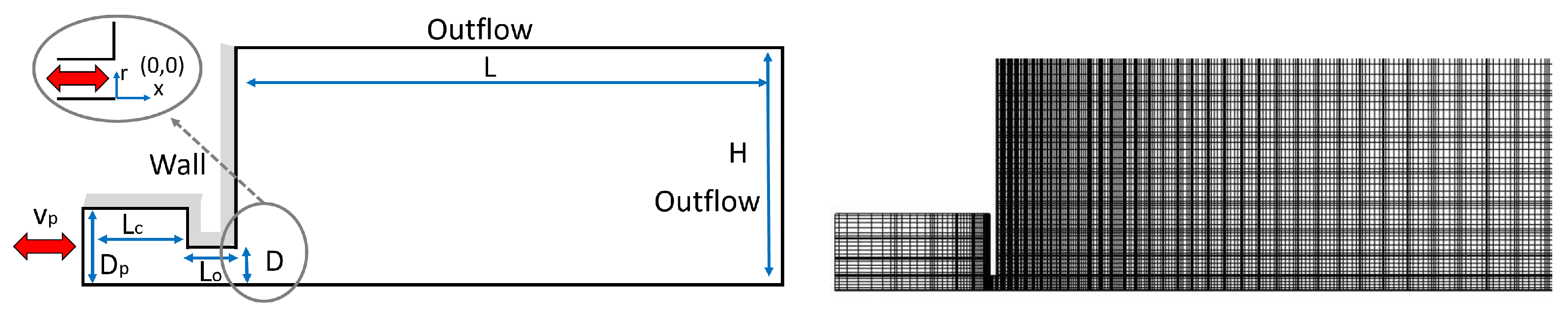
Figure 1 shows the computational domain of the numerical simulations, where axi-symmetric condition is imposed in the bottom side of the domain. The remaining boundary conditions and dimensions of the computational domain are set as in [30,34]. Regarding the dimensions of the domain: the diameters of the jet nozzle and the piston are set as and , respectively; the cavity length, jet stroke, cavity radius and jet orifice radius are defined as , , and , respectively; finally, to avoid boundary reflections the length and radius of the computational domain are set as and , respectively. Regarding the boundary conditions: the inlet boundary (piston) is defined as and for the streamwise and radial velocity components, respectively, and Neumann boundary conditions for the pressure; zero-stress and Dirichlet boundary conditions are imposed for the velocity ( = 0, with unit normal) and pressure (), respectively, in the top and outflow surfaces of the domain, while non-slip boundary conditions () are imposed in the wall of the jet and left surfaces of the domain.
A grid independence study and the validation of the numerical simulations with experiments have been carried out in [30]. The simulations have been performed varying the polynomial order as . The dominant frequency calculated in several points of the computational domain is St (similar to the experimental results) in the cases with and 10, varying in the 6th decimal digit, thus the polynomial order is set as .
3. The DMD-Based ROM: A Reduced Order Model Based on HODMD
Higher-order dynamic mode decomposition (HODMD) [24] is an extension of DMD [23] recently introduced for the analysis of noisy experimental data, non-linear dynamical systems and complex flows [35,36,37]. As with DMD, HODMD decomposes spatio-temporal data collected at time , , as an expansion of M Fourier-like modes as
where are the DMD modes, weighted with the amplitudes , oscillating and growing/decaying in time with frequency and growth rate . HODMD is a data-driven method, applied to analyze some data collected in the time interval to construct the previous DMD expansion. Nevertheless, for accurate calculations of such expansion, it is possible to either reconstruct the original data sequence (interpolation) or to predict temporal events (extrapolation), by means of adjusting the temporal term . This is the basic idea behind using HODMD as a ROM for data forecasting, with the aim at reducing the computational time in numerical simulations [25]. In other words, (i) a set of data are collected in the transitory of a numerical simulation, (ii) HODMD is applied to analyze the data and to construct the DMD expansion (4), (iii) to predict the attractor, only the permanent modes are retained to construct the previous expansion, these are the modes whose growth rate is close to zero (in the transitory all the modes either grow or decay in time, but the real dynamics is represented by a group of modes with relatively small growth rate, see [25]), (iv) the temporal term is adjusted to predict the attractor. A good way to select the permanent modes composing (4) is to establish a criterion based on a tolerance for the growth rates, thus the permanent modes are those whose growth rate is defined as . Once the DMD expansion (4) is constructed, the growth rate of such modes could be forced to be exactly equal to zero, , although for small values of , it is possible to maintain the real growth rate of such modes [26,27].
Algorithm
HODMD algorithm is briefly introduced in this section. A more detailed description can be found in Ref. [24]. For simplicity, before proceeding with HODMD algorithm, a group of K spatio-temporal snapshots are collected in the following snapshot matrix as
The dimension of the matrix is , with , being and the number of grid points defined along the streamwise and radial spatial components of the domain. The data are equidistant in time, with time interval . In this problem, each snapshot represents the velocity vectors and corresponding to the streamwise and radial spatial directions, organized in columns.
HODMD algorithm can be encompassed in three main steps.
- Step 1: SVD. With the aim at removing spatial redundancies or noise, SVD is applied to the snapshot matrix (5), aswhere the unit matrix, the diagonal of matrix contains the singular values , and is the reduced snapshot matrix, of dimension . Based on a tolerance (set by the user), it is possible to determine the number of N singular values retained in the previous equation, asAt this step, the spatial complexity of the data J is reduced to a set of N linearly independent vectors, determining the spatial dimension of the system, generally .In the analysis of complex data, SVD is replaced by a high-order singular value decomposition (HOSVD) [38], leading to the called multi-resolution HODMD algorithm. This decomposition organizes the original snapshot matrix in tensor form as , with being the number of velocity components ( and ), for ; and . HOSVD algorithm applies an SVD to the three matrices whose columns are formed by each one of the 3 data variables (similar to the fibers of a tensor). Thus, this method provides the following decomposition for each velocity component l (for simplicity the solution is particularized for a single velocity component)where is a third-order tensor (called the core tensor) and the columns of the matrices , and are known as the modes of the decomposition (two spatial and one temporal modes, respectively). The rank reduction in Equation (7) is then applied to each one of these modes. The temporal modes are used to construct the reduced snapshot matrix. Due to the complexity of the data analyzed in this article, this multi-resolution algorithm is used to construct the DMD-based ROM (see more details about the algorithm in [14]).
- Step 2: the DMD-d algorithm. DMD algorithm [23] is combined with the Takens’ delay embedding theorem [39], providing the following high order Koopman assumption that is applied to the reduced snapshot matrix asThe dynamics of the system is contained in the reduced Koopman operators , , ⋯, . These operators are encompassed into a single matrix. The eigenvalues of such matrix provide the frequencies and growth rates of the DMD expansion (4), and the eigenvectors are used to construct the DMD modes . It is remarkable that for values of , this algorithm is similar to standard DMD [23], providing similar solutions. Nevertheless, in the analysis of complex dynamical system, composed by large number of frequencies, transient modes, or even noisy data, values of will provide accurate approximations of the expansion (4), required to construct a ROM and to predict the attractor (note that the errors grow exponentially with time).
- Step 3: Amplitude calculations and RRMS error. The amplitude weighting the DMD modes are calculated in this step. For proper reconstruction of the original data (interpolation), a good way to calculate the amplitudes is by least squares fitting of the expansion (4). This amplitude will determine the number of M DMD modes retained in the expansion as function of a second tolerance , asOnce the DMD expansion (4) is approximated, the relative root mean square error (RRMSE) is used to quantify the difference between the original data and the approximated solution (4), aswhere represents the Frobenius norm.To minimize this error, the method is applied iteratively. In other words, the algorithm is applied over the solution reconstructed in (4), obtaining new reconstructions, until the number of singular values N is maintained similar in two consecutive iterations. It is possible to download a MATLAB [40] version of the HODMD algorithms in Ref. [41].
4. The DMDlr-ROM: A Low-Rank Spatial Approximation for the Data-Driven ROM
Generally, the storage and analysis of databases describing complex or turbulent flows implies using sophisticated and powerful computers. The size of each snapshot composing the snapshot matrix (5) varies from a few megabytes to hundred gigabytes in data generated in numerical simulations describing turbulent flows [28], making prohibitively expensive using HODMD algorithm for the analysis of flow structures. This section presents a low-rank approximation of the snapshot matrix (5) to construct the data-driven ROM based on HODMD previously introduced, which will reduce the computational cost. This new algorithm, presented for the first time in this article to the author knowledge, is known as DMD low-rank ROM (DMDlr-ROM). The methodology can be encompassed in three main Stages.
- Stage 1: rank reduction and generation of the new snapshot matrix. SVD is applied to reduce the spatial dimension of the original snapshots. In contrast to Step 1 from HODMD algorithm, SVD is applied separately to each one of the snapshots composing the snapshot matrix (5). Thus, the information contained in each snapshot is organized in tensor form as for and . For each snapshot k the SVD leads aswhere the dimension of is , the dimension of is and the dimension of is . This decomposition has been carried out using the function svd in MATLAB [40]. The spatial matrices and contain information related to the streamwise and radial spatial components, respectively, and is the matrix containing the singular values . The spatial matrices are weighted with the square root of the singular values asandbeing the matrix composed by the square root of the singular values .The same process is repeated for each one of the K snapshots of the initial snapshot matrix (5) for each velocity component and . Two new snapshot matrices are constructed with the results previously obtained, the called X-snapshots defined asand the called Y-snapshots, defined asIt is remarkable that matrices (15) and (16) are composed by sub-matrices of dimension and , respectively, thus the most efficient way to organize this information is in tensor form as and , being the variable defining the number of singular values, for . For each velocity component l the previous expressions lead as and .The reduction of memory size in the previous snapshot matrices is dependent on the number of singular values N retained in each one of such matrices. To ensure the proper performance of the model proposed, N can be determined according to a certain tolerance, as in Equation (7), or simply by identifying changes in the tendency of the singular values obtained in the SVD analysis carried out for each snapshot.
- Stage 2: modal decomposition using HODMD. The multi-resolution HODMD algorithm is applied to each one of the tensors obtained in the previous step, and . The following DMD expansion is obtained for the X-snapshots (for simplicity particularized of one velocity component)and for the Y-snapshots (for one velocity component)where and are the DMD modes retained for each expansion, and are the amplitudes and and are the DMD modes. Please note that the number of modes composing each expansion can be different, meaning that the amplitude of each mode describing the dynamics of the system varies in each analysis.
- Stage 3: temporal predictions and data reconstruction. The attractor is predicted by simply adjusting the time as in (17) and (18). Then, the new data predicted by the previous models are reconstructed as (for each velocity component)in matrix form defined aswhere the dimension of is and the dimension of is .As previously mentioned, the number of DMD modes defining each spatial matrix can be different, since the amplitude of the most relevant flow dynamics varies in the spatial domain. Thus, for some groups of tolerances , it is possible obtaining DMD modes defining expansion (17) and modes in expansion (18). Similarly, for some tolerances it is possible that and . Depending on the complexity of the data analyzed, and the influence of the global dynamics related to each spatial direction, a good alternative to reconstruct the solution predicted in time is using the following expansionwhere is the tensor obtained in Stage 1 of this algorithm. Similarly, the predicted solution could be reconstructed aswhere is the tensor obtained in Stage 1.
5. Generating Artificially the Optimal Vortex: A Way to Predict the Perfect Set-Up in Synthetic Jets
This section presents a new theoretical and simple approach suitable to predict the artificial generation of the optimal vortex using synthetic jets. Gharib et al. [6] identified the formation number to generate the optimal vortex as for values of Re . These authors also relate such number with the running mean of the piston velocity and the piston oscillation period as
Thus, it is possible to relate with the oscillation frequency and the formation number as . The oscillatory movement of the piston can be approximated by a simple sinusoidal function, encouraging the flow to continuously leave and re-enter into the cavity, as presented in Section 2. Since this function is even (zero net mass flow), the proper way to define the piston oscillation velocity is considering half of the oscillation period (), as
It is remarkable that these authors identified the piston velocity as the velocity scale defining the flow dynamics, nevertheless the present article considers the mean flow velocity leaving the jet nozzle as the characteristic velocity scale of the flow (see more details in Refs. [14,15,30]).
Gharib et al. [6] introduced the definition of the running mean of the piston velocity as
Following the work presented in [14,15,30], as introduced in Section 2, the piston velocity varying with time is defined as . Introducing this equation into (25), leads to the following integral, defining the piston velocity in half period of the oscillatory movement as
Comparing terms in Equations (24) and (26), it is possible to obtain the following expression for the frequency
This value defines the optimal oscillation frequency of the piston required to generate the optimal vortex, which depends on the jet nozzle diameter and the amplitude of the piston oscillations.
To relate this solution to the bifurcation diagram presented in Ref. [15], it is necessary to calculate the frequency in terms of the non-dimensional Strouhal number, defined in Section 2 as . The characteristic velocity scale is defined by the mean flow velocity leaving the jet nozzle, which was related with the piston velocity and dimensions in Equation (3) as . Taking into account the relationship between the diameter of the piston and the jet nozzle, defined as , it is possible to approximate the mean flow velocity as
This expression defines a way to calculate the (non-dimensional) frequency required to generate artificially an optimal vortex using synthetic jets with rounded cavity and nozzle, depending on the amplitude of the piston velocity and the diameter of the jet nozzle. Generally, for non-dimensional values, the jet diameter is set as , thus the previous expression only depends on the piston velocity amplitude.
For values of the frequency is St (regime(i) in Ref. [15]). On the contrary, if then the frequency is St (regime (ii) in Ref. [15]). As seen, the efficiency of the system is defined by the amplitude of the piston oscillation, which is in good agreement with the quantity of energy necessary to produce such amplitude, using for instance an engine. The artificial generation of the optimal vortex assumes amplitude values as (minimizing the quantity of external energy), meaning that the oscillation frequency required to generate such optimal vortex is St ≃ 0.022. This result is in good agreement with the bifurcation diagram presented by Carter & Soria [15] and the experiments carried out by Daribi et al. [16]. On the one hand, Figure 5 in Ref. [15] shows that for values of Re and St the flow regime is described by a laminar jet (regime (i)), while for values of St the flow regime is conformed by vortex rings (regime (ii)). From these experimental results it is possible to guess that the transition point between these two regimes is defined by Strouhal values defined in the interval St . On the other hand, when Daribi et al. [16] studied in detail the swimming motion of 7 types of jellyfish, the authors showed that the most efficient jellyfish were producing a jet stream defined in regime (ii) (St ), while the highest impulse was generated by the jellyfish producing a jet stream defined in regime (i) (St ). This result connects system efficiency with the energy introduced to the system, by means of controlling the piston oscillation amplitude. As seen, the generation of the optimal vortex lies in the transition between regions (i) and (ii), meaning that this vortex will produce the highest impulse using the minimum amount of energy possible. Increasing the frequency to values larger than will lead to energetic rises coming from the higher amplitude of the piston oscillation required to generate the vortex, and consequently diminishing the system efficiency.
Finally, it is remarkable that the formation number given by Gharib et al. [6] was calculated for values of Re (these authors defined the Reynolds number as function of the vortex circulation as , which is equivalent to Re using the jet nozzle diameter and the jet nozzle mean flow velocity as characteristic scales). As explained by Bandyopadhyay & Beal [22], the frequency is not the only parameter that guarantees the presence of the optimal vortex. Thus, based on practical experience, to guarantee the generation of the optimal vortex it is necessary to follow the diagram by Carter & Soria [15] and to fix the Reynolds number within the interval Re . The results presented in such diagram show that for values of Re , the transition point is always located in the interval St , suggesting that St is the critical value to generate the optimal vortex. Please note that the equations presented in this section related to the formation number were formulated for Re ; however, the Reynolds number of the results presented in the numerical simulations is Re , which confirms that these equations are valid for smaller Reynolds numbers, showing that the optimal vortex is generated for values of St and Re .
The artificial generation of the optimal vortex has been studied in detail comparing numerical results with the previous theoretical approach. Figure 2 compares the topology patterns of three different test cases calculated at Re , these are St (regime (ii)), St (critical value) and St (regime (i)). The figure shows contours of instantaneous spanwise vorticity and the streamlines describing the vortex ring in the jet flow at a representative time instant of the injection phase, when the vortex ring leaves the cavity. As seen, at St it is possible to distinguish two different vortex rings ejected from the cavity, while at St a single vortex ring followed by a laminar jet with a well-defined structure is clearly identified. The transition between these two regimes is clearly shown at St , where a single vortex ring leaving the cavity is followed by a small vortex in a continuous structure, suggesting the presence of a laminar jet.
6. A ROM to Predict Spatio-Temporal Flow Structures in Synthetic Jets
This section presents a data-driven ROM based on HODMD that predicts spatio-temporal structures in synthetic jets. The main goal of this model is to approximate solutions converged in time from a reduced number of snapshots collected in the transitory region of a numerical simulation, when the solution is still continuously changing due to the presence of many non-permanent modes, decreasing in time. The model has been tested using four different configurations of the database generated from the numerical simulations calculated at St . Due to the presence of flow instabilities in the laminar jet stream combined with the flow instabilities related to the periodic vortex ring ejected from the cavity [30,31], this test case is the most complex of the three test cases simulated. Nevertheless, as it will be shown below, the versatility of this method makes that this tool can be successfully applied to construct ROMs in the data obtained at St and obtaining similar results (similar speed-up factor and RRMS error, not shown on this paper for the sake of brevity). Two different models will be presented below. In the first case, the standard DMD-based ROM is applied to predict the flow features in synthetic jets, with the aim at showing the good performance of this technique to predict spatio-temporal data in this type of problems. In the second case, the novel approach DMDlr-ROM is applied to predict the previous spatio-temporal flow structures, using only the 30% of the total memory necessary to solve the initial problem with the DMD-based ROM, and reducing the computational time in the generation of the model by a factor of ~3.
6.1. Predictions Using the DMD-Based ROM
In all the cases presented, a group of K snapshots, equidistant in time with are collected starting at time , thus they are defined in the time interval , with . The number of piston cycles contained in each snapshot group is given by , with being the period of each oscillation. The parameters used for each HODMD analysis are and the value of d is adjusted proportional to the number of snapshots collected in each case as (the value of the tolerances and d is based on the results presented in [30,31]). In all cases, the DMD expansion (4) is constructed to create a ROM. The temporal term is then adjusted to time , representing the 10th cycle of oscillation. Then, the solution is predicted 15 more cycles, up to time . The speed-up factor of the numerical code is measured with the ratio . Table 1 summarizes the analyses carried out and includes the number of DMD modes retained in each case, being and M the total number of modes and the number of permanent modes, respectively, which are defined in this example as the modes with growth rate , with and . The RRMSE made in the prediction of the 15 time intervals in the near and far fields and in the complete field are represented by RRMSE-N, RRMSE-F, and RRMSE, respectively.
As seen, the number of permanent modes retained in the DMD expansion (4) increases with the number of snapshots used in the analysis. This explains that the model predicts the real solution with smaller errors, although it is necessary to assume a penalty in the speed-up factor of the code. Moreover, increasing the number of snapshots in the original data analyzed, also increases the complexity in the DMD analysis meaning that for large three-dimensional databases representing complex flows (i.e., transitional or turbulent flows), it could be necessary to combine HODMD with the low-rank strategy to reduce the spatial dimension of the data, as it will be presented in the next section. The error made in the predictions of the data is larger than 60% in Models 1 and 2 and ~34% in Models 3 and 4, with the exception of Model 4 using predictions with and , where the error is larger than 55%. The RRMS error in the near field of Models 3 and 4 is ~23%, meaning that the performance of the model is better predicting the near field than the far field. The speed-up factor in Model 3 is , while in Model 4 , suggesting that Model 3 is the best model for temporal predictions in synthetic jets. It is remarkable the large RRMS error made in these calculations, ~34%, nevertheless, the main goal of this DMD-based ROM is to predict the global dynamics representing the main temporal patterns describing the flow and the evolution of the periodic ejection of vortices. As it will be seen below, the model perfectly predicts the general dynamics driving the flow in synthetic jets, represented by the large size flow structures. Increasing the snapshot number, and collecting data in the permanent region of the numerical simulations, will diminish the RRMS error providing information related to the small-size flow scales; however, this will substantially increase the computational cost of the simulations. This work presents a balanced relationship between minimizing the error in the data predicted while minimizing the computational cost of the simulations. Although it is possible to diminish the RRMS error of the data predicted using lager number of snapshots paying a small penalty in the speed-up factor of the code (i.e., Model 4 compared to Model 3), the accuracy in the prediction of the large size flow structures will be kept almost invariant (the error is slightly reduced, some clarifications will be presented below), suggesting that it is better to assume the error with the aim at obtaining large benefits related to the reduction of the computational time.
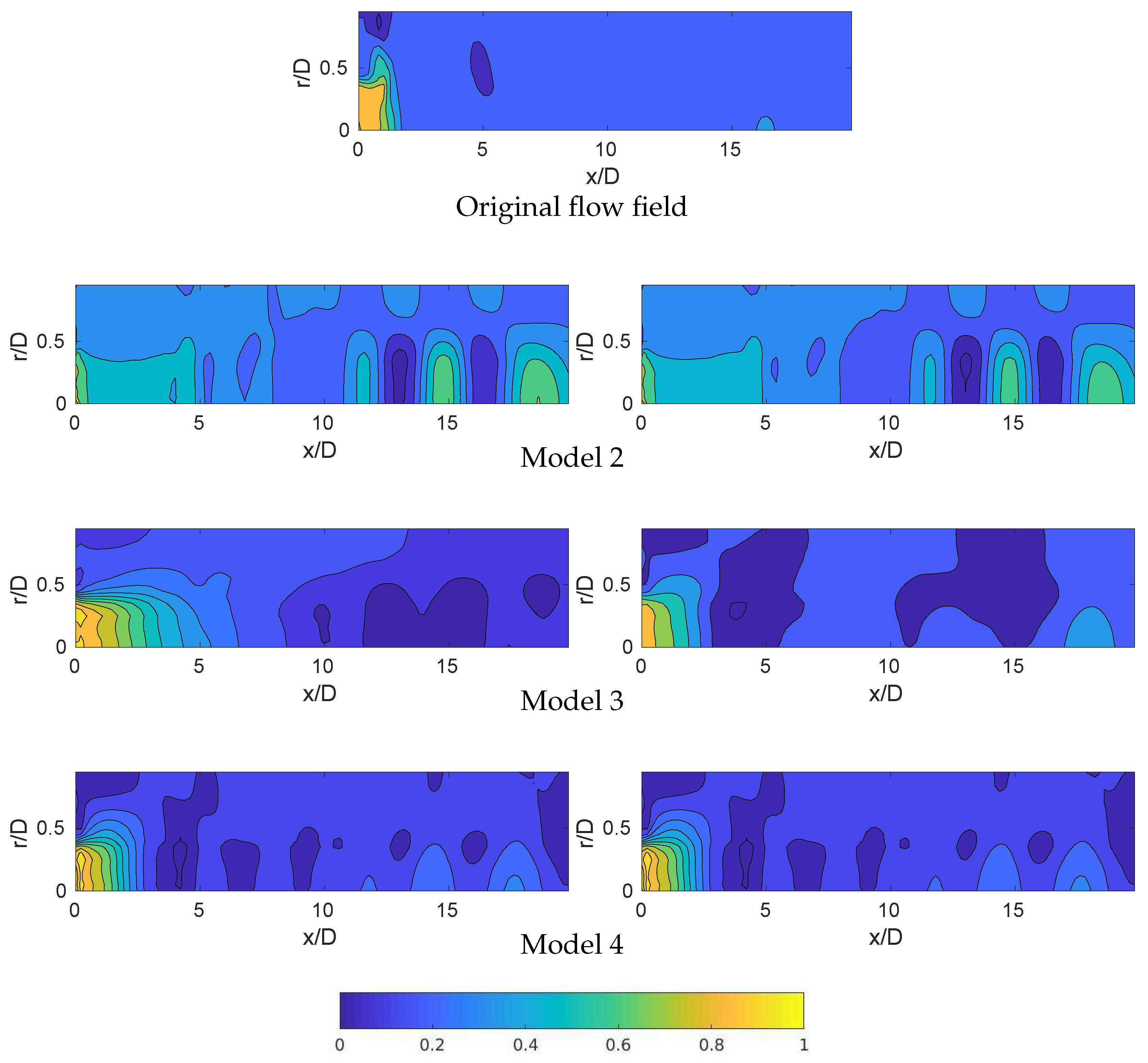
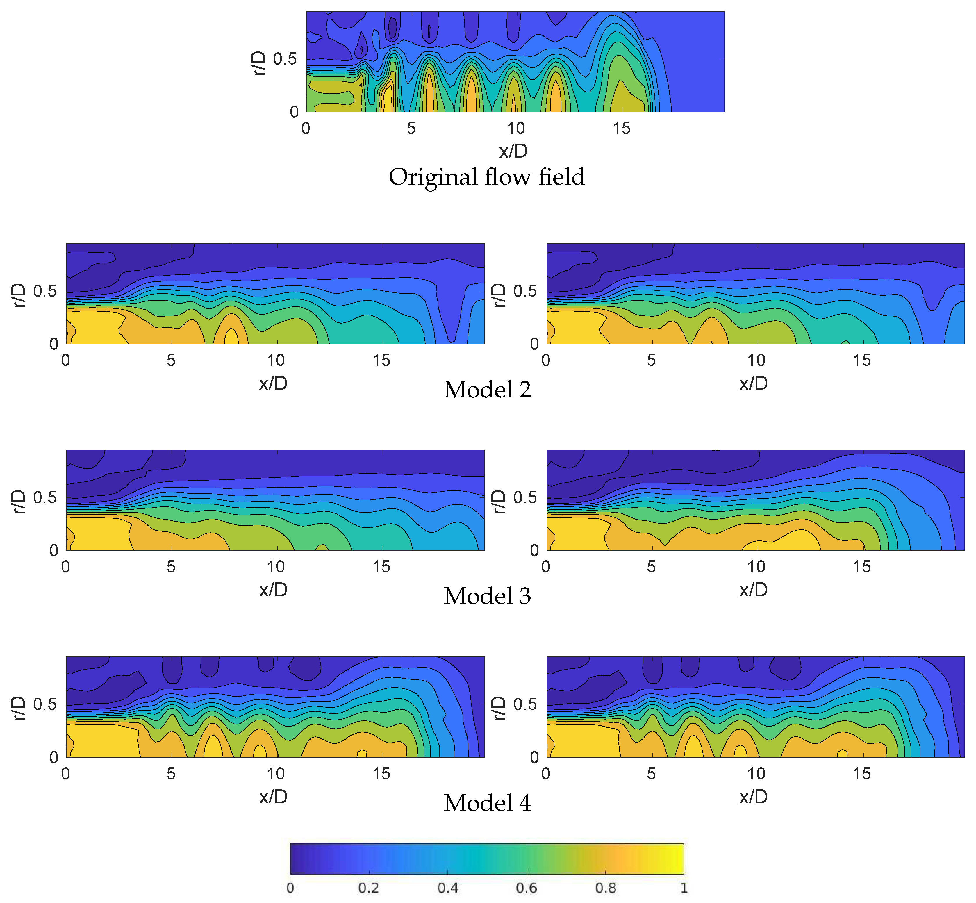
Figure 3 and Figure 4 compare the original solution at time and with the predictions carried out in Models 2, 3, and 4. The results for Model 1 are omitted, since they are completely spurious, nevertheless the remaining cases succeed in the prediction of the large flow structures. The smallest flow structures, identified in the original data as small spatial elements (that could be compared with noise), are missing in all the DMD-based models. The jet flow structures in the near and far field are better represented by Model 4 than Models 2 and 3, being the representation of Model 3 better than Model 2. In the results provided by Model 4, it is possible to distinguish (i) the small-size element leaving the jet cavity, related to the vortex ring, and (ii) a group of medium-size structures in the far field, , possibly related with high-frequency temporal patterns. The presence of these structures is attenuated in Model 3, especially in the case with , and in Model 2, where the wake of the jet start vanishing at spatial positions and the near field of the jet is not properly represented.
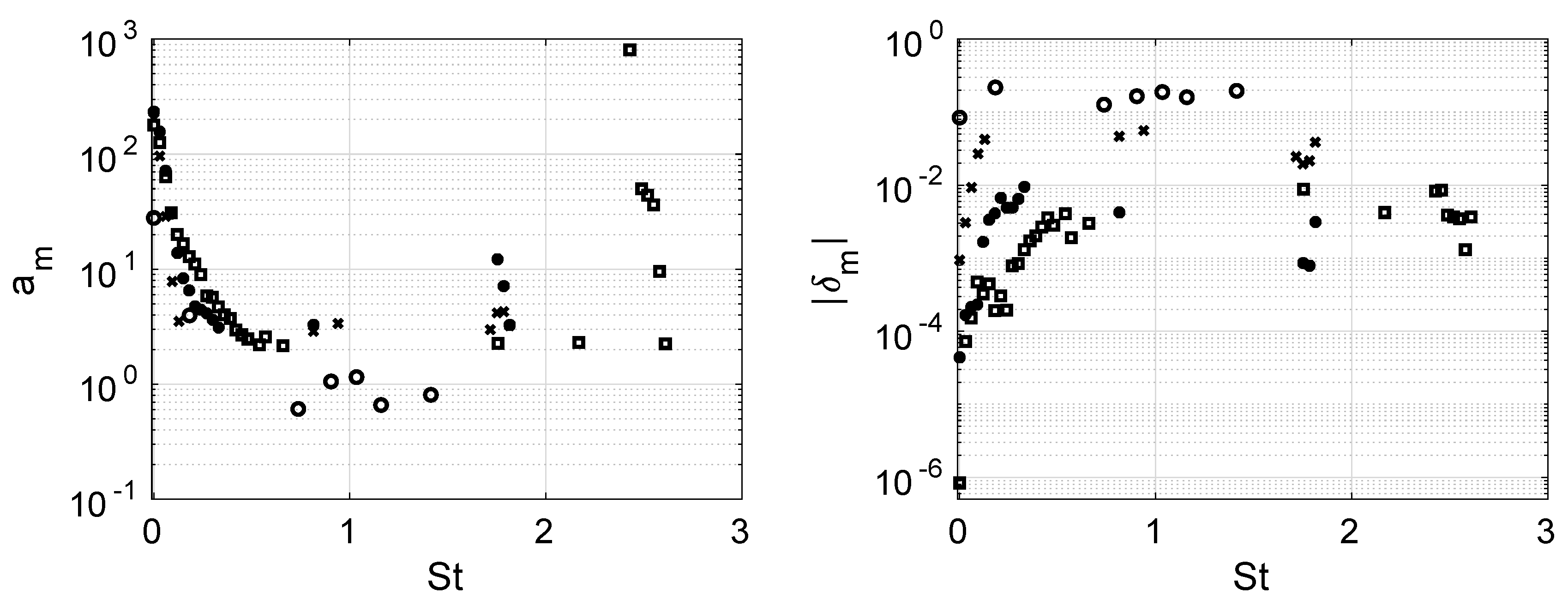
Figure 5 compares the frequencies vs. amplitudes and growth rates calculated in Models 1, 2, 3, and 4. The method retains a group of low-amplitude high-frequency spurious modes in Model 1, on the contrary, the remaining models retain a group of periodic modes, with leading frequency St (forcing frequency), representing the general dynamics of the flow (see [14] for more details). The main differences found in these analyses lies in the (i) calculations of the growth rates, defining the accuracy of the frequency values (the more accurate, the smaller growth rate), showing that the modes are better calculated in Model 4, followed by Model 3 and Model 2, and in (ii) the number of high-frequency modes retained, which represent the flow physics of the far field, related to the small-size periodic flow structures identified in Figure 4. Model 4 retains a larger number of high-frequency modes than Model 3 and Model 2, explaining the better performance of the former model. Nevertheless, the RRMS error in the total interval predicted , is very similar in Models 3 and 4, suggesting that both models perfectly predict the general dynamics in synthetic jets for large time periods.
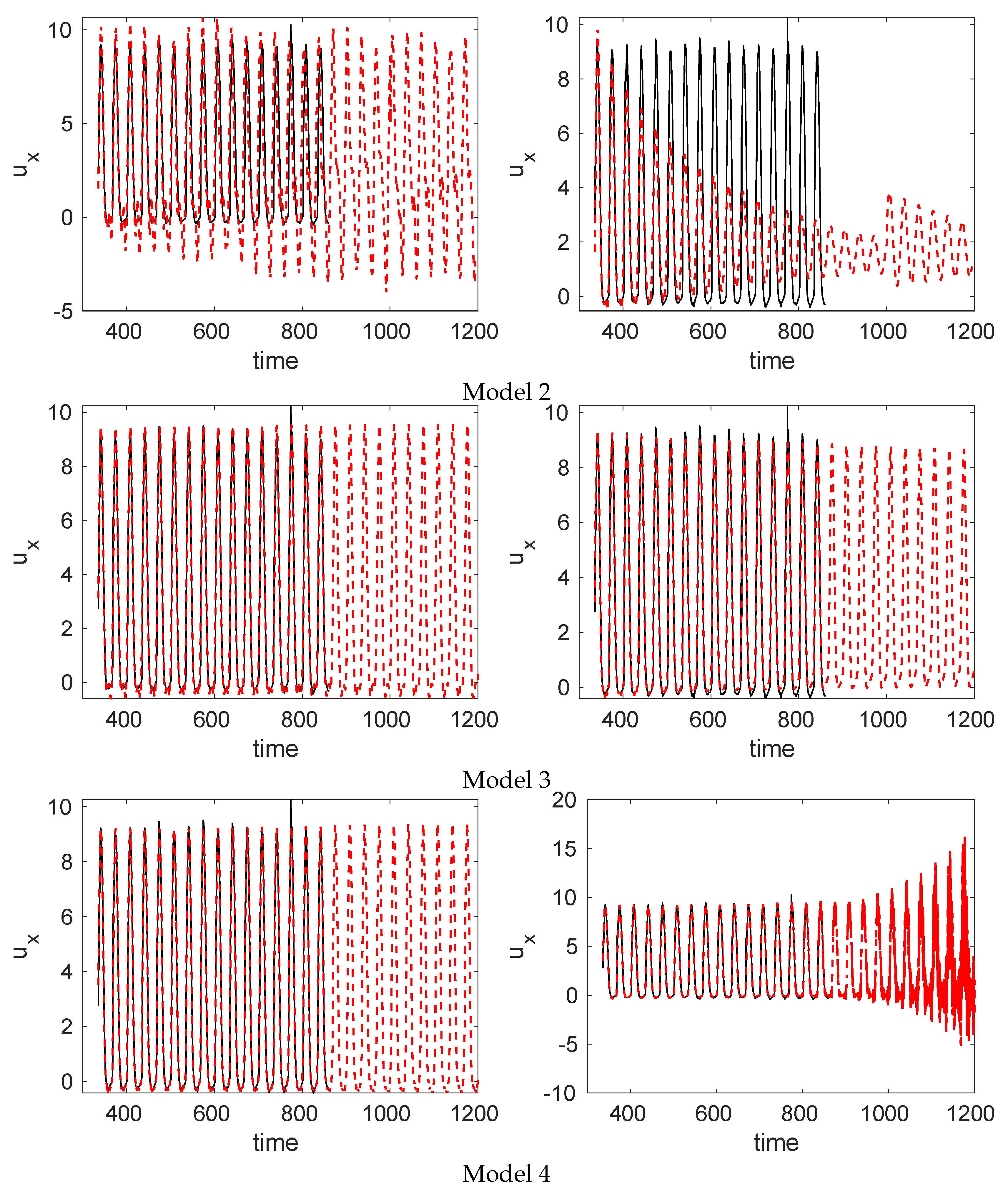
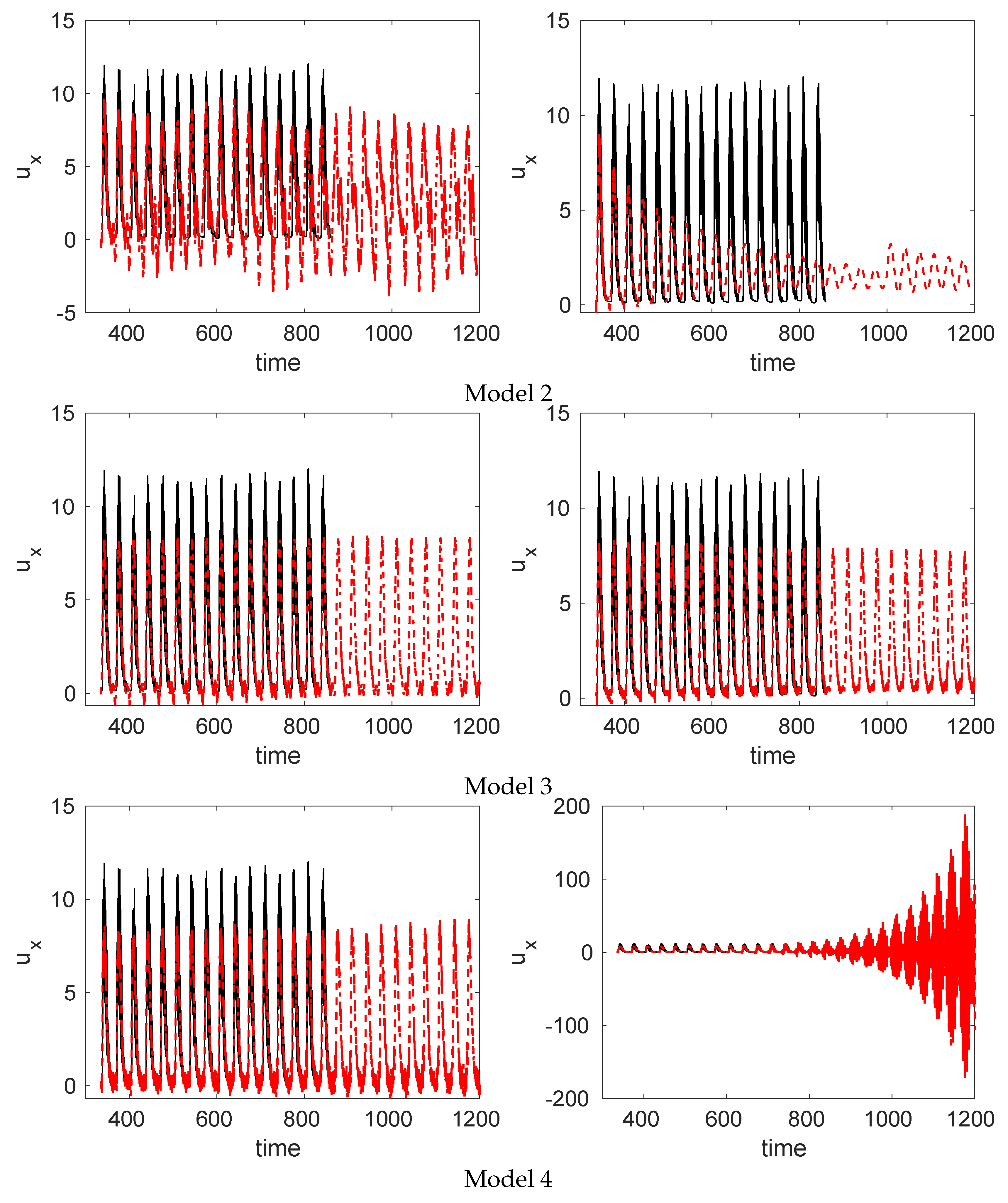
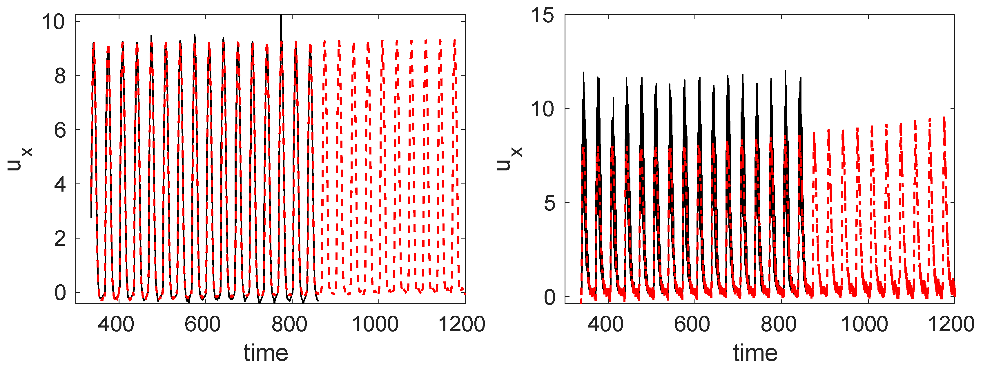
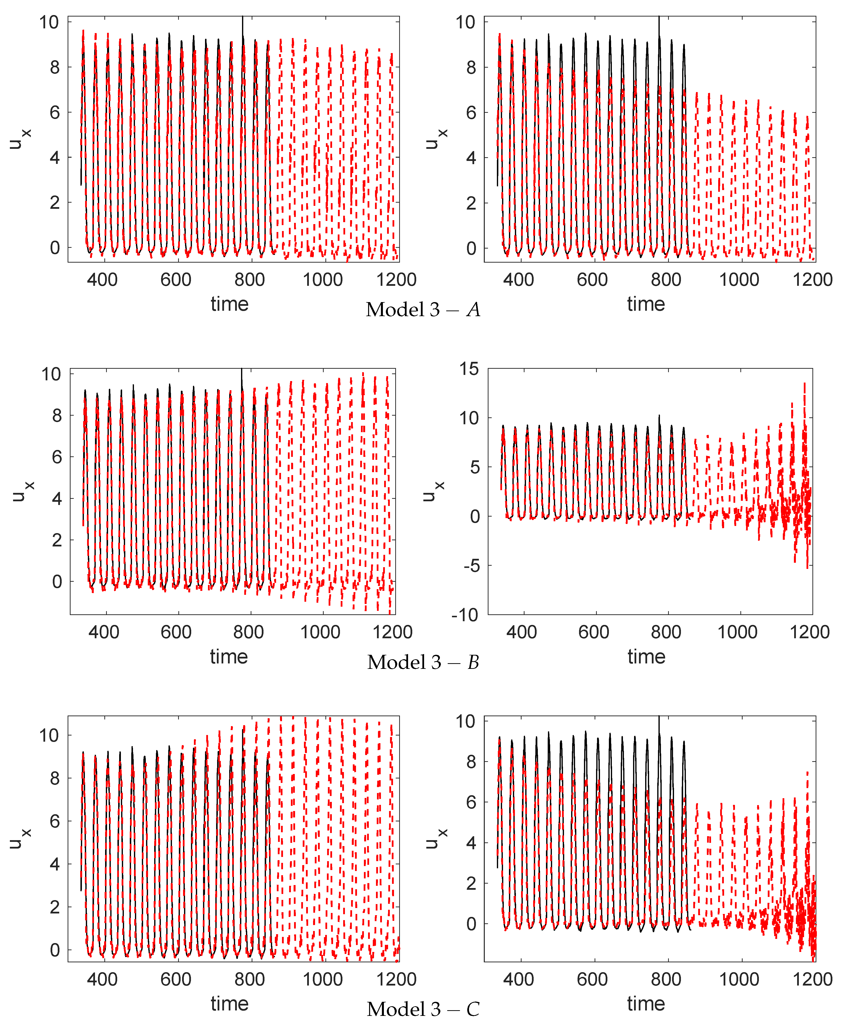
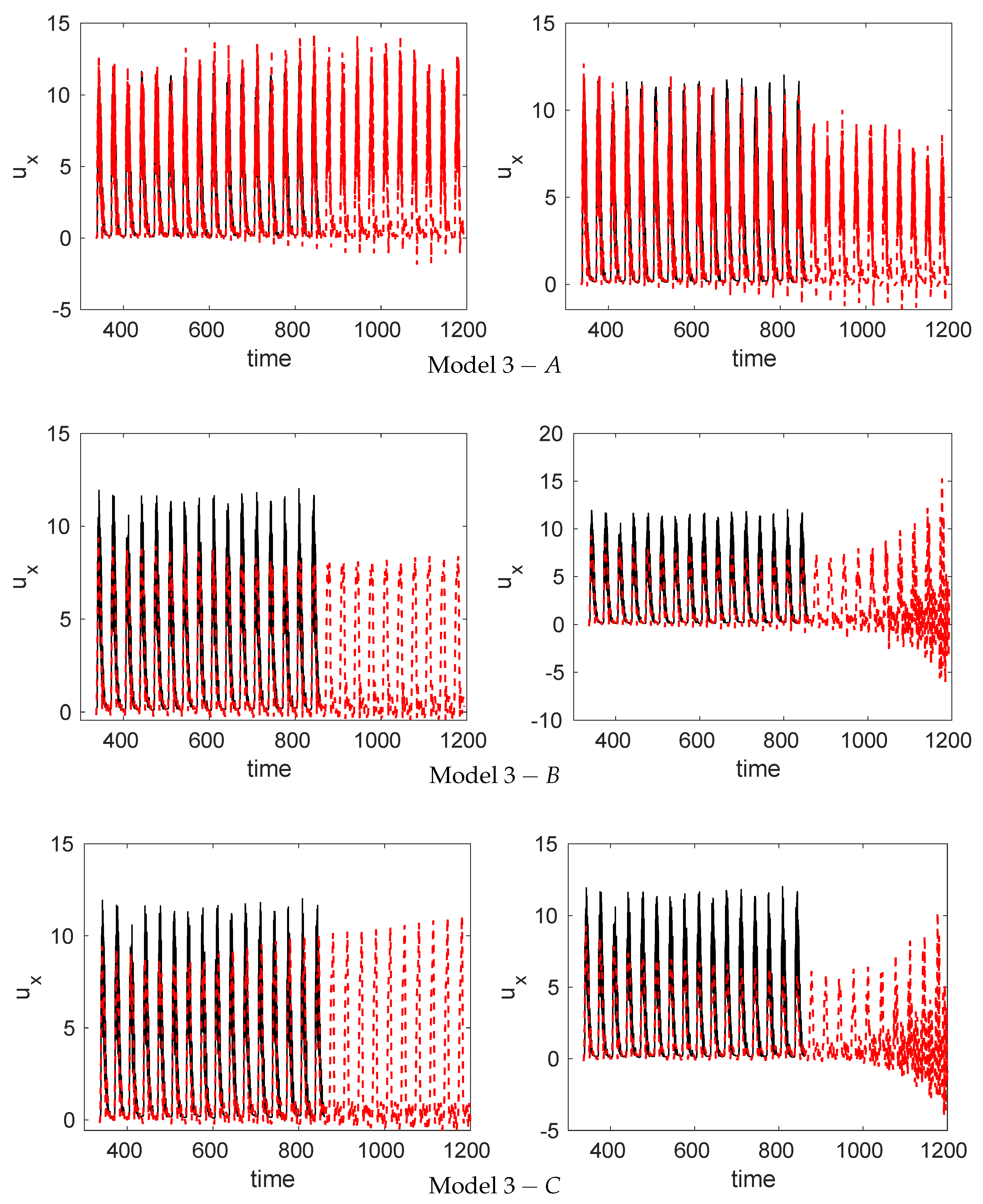
The temporal evolution of Models 2, 3, and 4 is compared with the original solution in Figure 6 and Figure 7 in two representative points of the computational domain, extracted in the near and far fields. As predicted by the RRMS error (>60%), Model 2 fails in the prediction of the 15 cycles, while models 3 and 4 perfectly predicts both the near and far fields up for 26 cycles (from cycle 10 to cycle 36), with the exception of Model 4 using and , whose solution diverges in time. It is possible to overcome such problem using instead, as shown in Figure 8, where Model 4 provides similar solutions as Model 4 with and Model 3.
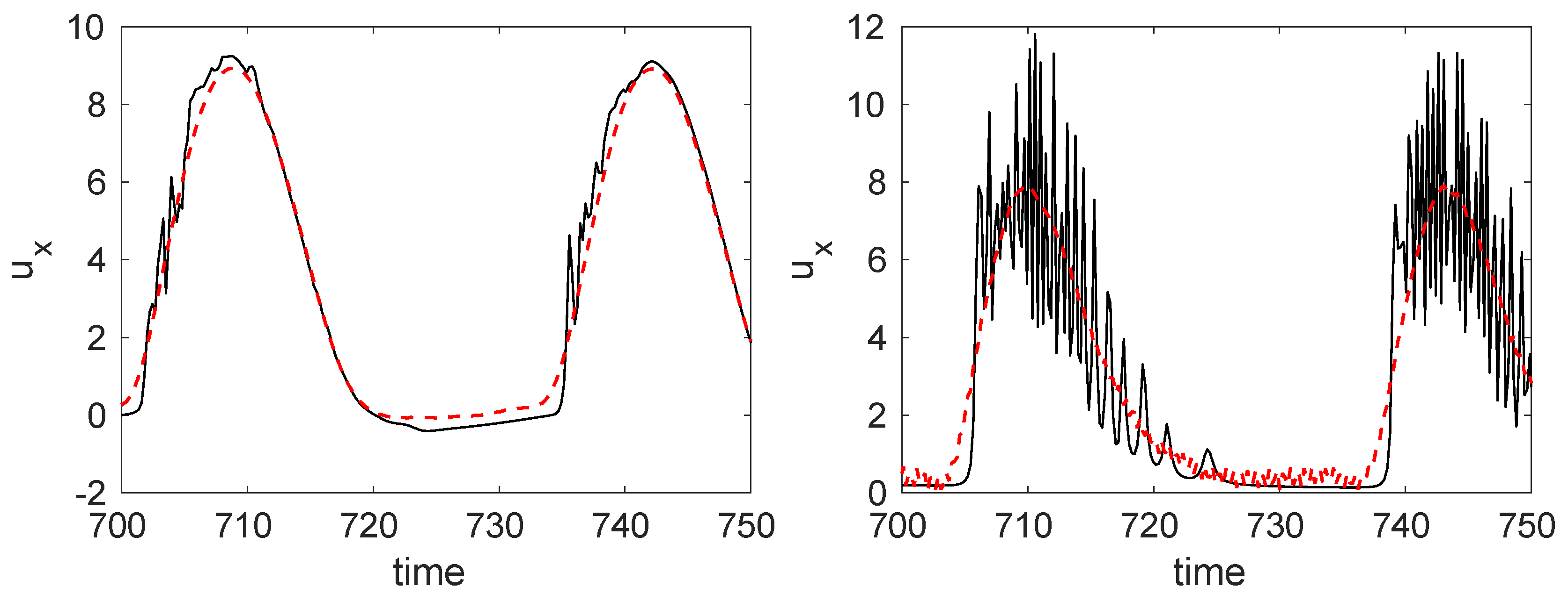
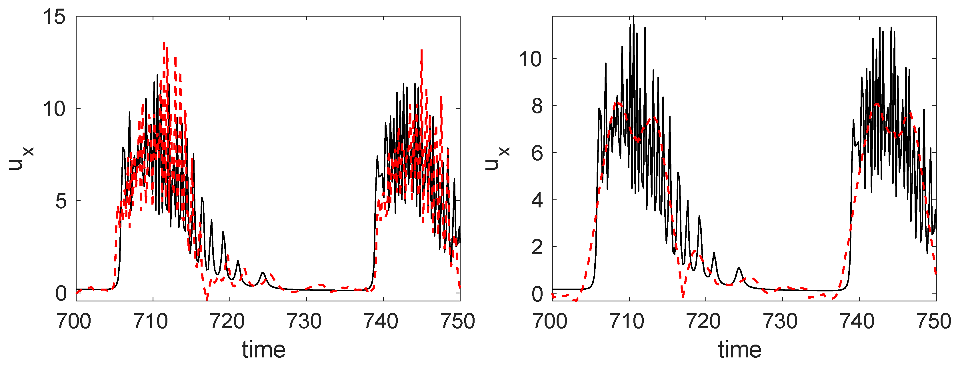
The previous figures suggest that the qualitative error made in the calculations of the flow structures in the near field is smaller than 23%, and in the far field is smaller than ~34%, as predicted in the RRMSE calculations presented in Table 1. Thus, the high value presented in such calculations could be related with the small-size flow structures defining the flow. This fact is confirmed in Figure 9, comparing the real solution with the velocity fields predicted in the near and far fields in cycle 22 (predictions up to cycle 25). The general dynamics, the large size flow scales, are predicted with RRMS error smaller than 3% (calculated with the flow field averaged in time); however, the method is not able to predict some very high-frequency flow oscillations, related with low-amplitude/small-size flow structures or with the medium-size structures describing the wake of the jet. This fact confirms the good performance of Model 3 as a DMD-based ROM to predict large size flow structures in synthetic jets with speed-up factor of and errors smaller than 3% in the streamwise velocity. Please note that the smaller size structures could be predicted with smaller error (i) using larger number of snapshots, with smaller temporal distant to construct the snapshot matrix (5) and (ii) using information of the numerical simulations converged in time, but these two steps will increase the computational cost of the ROM and will not provide additional information of the general flow dynamics, which is the main scope of this paper, although it remains as open topic for future research. Finally, it is remarkable that similar results are found for the normal velocity component, not shown for the sake of brevity, since such vector field is one order of magnitude smaller than the streamwise velocity field.
6.2. Efficient Computations Using the DMDlr-ROM
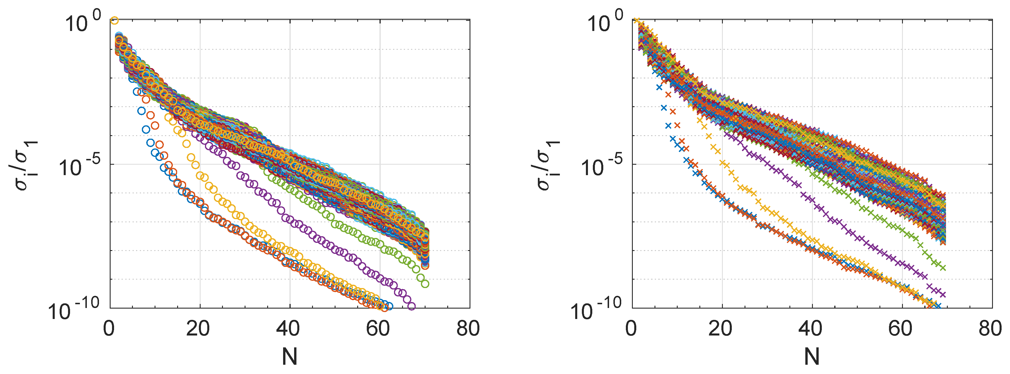
The previous section shows that Model 3 provides a good general approximation of the flow field in the temporal predictions carried out, thus this is the model selected to perform the low-rank approximation to construct the DMDlr-ROM. The parameters set for the DMD analysis are listed in Table 1 (snapshot number K, d, , and for Model 3). Before starting with the DMD analysis, it is necessary to set the value of N singular values that will be retained to construct the X-snapshot and Y-snapshot tensors (15) and (16). Figure 10 shows the evolution of the singular values calculated in 1873 snapshots. A clear change of tendency is observed in a few snapshots for values of , while this change of tendency is observed in the remaining snapshots for values closer to . To ensure the proper performance of this ROM, the number of singular values is set as . The size of the snapshot matrix is reduced by ~70%, from Gb to 472 Mb and 330 Mb for the X-snapshot and Y-snapshot tensors, respectively, and the computational time required to construct the model is also reduced by ~70%, from to seconds for each case.
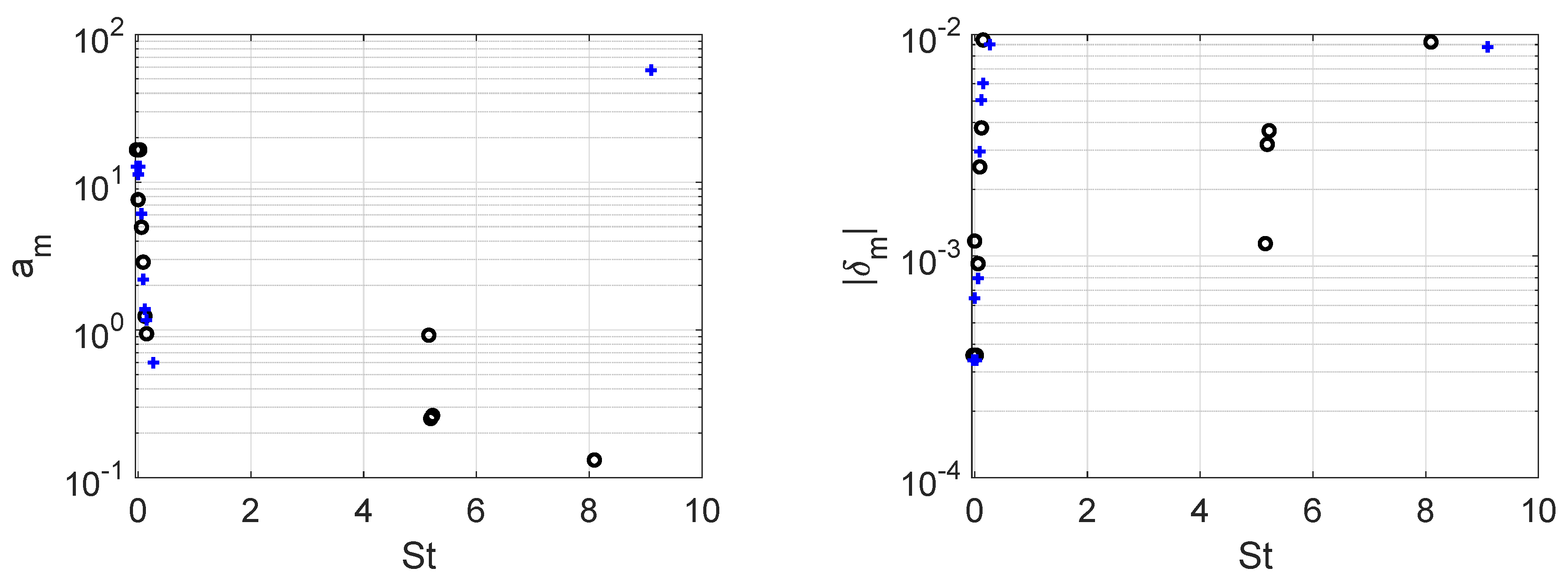
HODMD is applied using the tolerances retaining 19 and 0 modes in the expansions (18) and (17), respectively, suggesting that the X-snapshot tensor (15) is related with smaller amplitude modes. Thus, the same analysis is carried out to such tensor, using the tolerances and , retaining 15 modes. The frequencies vs. amplitudes and growth rates calculated for each analysis are compared in Figure 11.
From the 15 modes calculated in the X-snapshot tensor (low tolerances), 12 of them represent the periodic modes with leading frequency St , one of them represent the steady mode with zero frequency, and the two remaining modes are related with high frequencies, decaying in time with growth rate ~10−2 (note that the modes include their complex conjugate counterpart). On the contrary, in analysis of the Y-snapshot tensor (high tolerances), the method retains 10 periodic modes, the zero-frequency mode, and a group of high-frequency modes. This fact suggests that the high-frequency spatio-temporal structures found in the wake of the jet, shown in Figure 4 presents higher amplitude in the data represented in the Y-snapshot tensor.
The predictions of the flow structures in the time interval are carried out using expansions (17) and (18), and the data are reconstructed using the three different models defined by Equations (19), (21) and (22). Table 2 presents the RRMS error made in the predictions of the near and far fields and the complete flow field. The error made in the results presented in Model using is smaller than ~25% in both the near and far field calculations, improving the results obtained in the previous section, without any rank reduction. This model predicts the spatio-temporal flow structures only considering the temporal variations found in X, related to the low-amplitude modes, mainly represented by the periodic modes with leading frequency St . On the contrary, the largest errors are found in Model , which considers the variations in time of the X and Y spatial components. This fact suggests that the complex flow patterns describing the vortex ring and the wake in synthetic jets is related to small amplitude variations in time along the streamwise direction, while the temporal variations along the radial component remain almost constant.
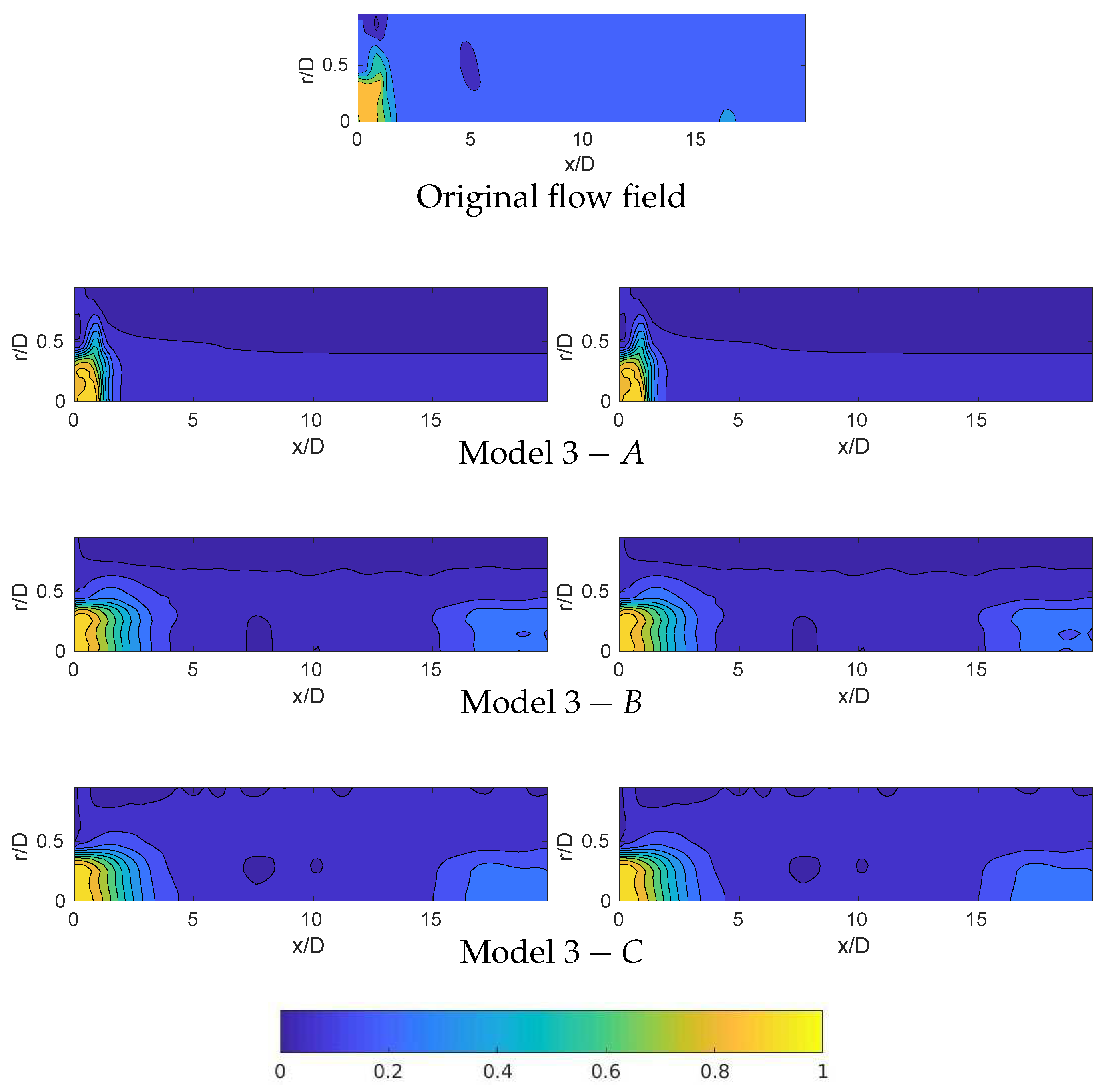
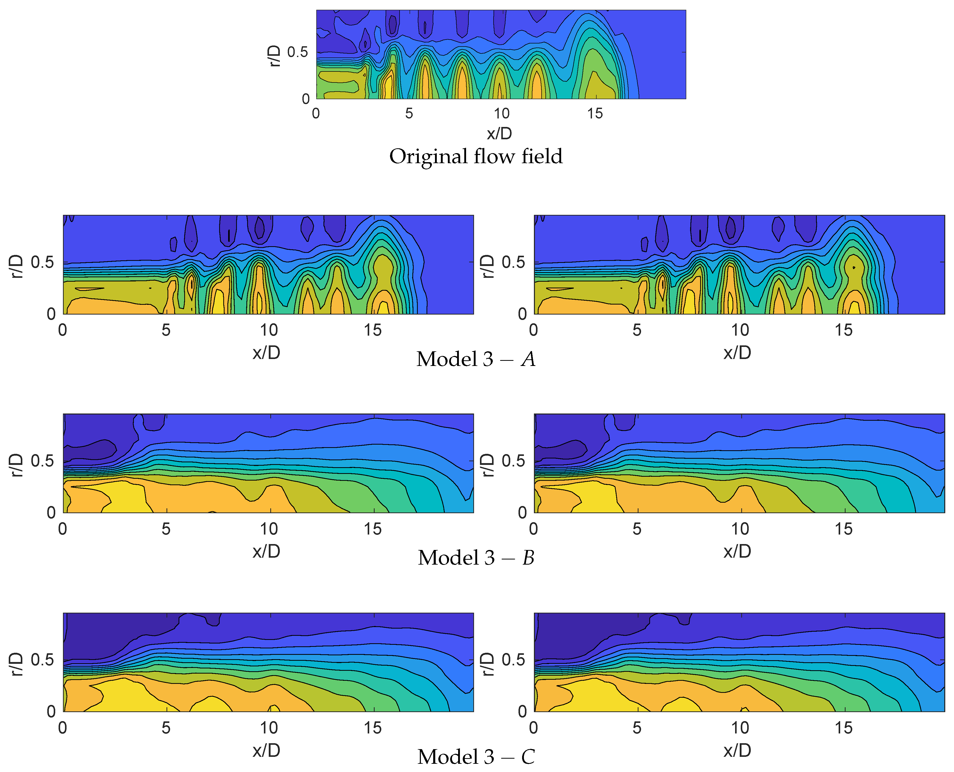
Figure 12 and Figure 13 compare the streamwise velocity contours of the original flow field with the solution obtained with Models , , and . The figures show qualitatively the good performance of the three models to predict the large size flow structures, and especially Model , which also predicts the medium-size structures in the wake of the jet.
The temporal evolution of these three models is shown in Figure 14 and Figure 15. In contrast to Model 3 presented in the previous section, the performance of these low-rank approximations is better using in the permanent modes. For values of , all the models diverge as time passes by. Regarding the models with , the best performance is described by Model , whose predictions could be extended up to time 1200 (36 cycles). The performance of Model is also good, although this model starts slowly diverging after cycle 25. Finally, Model slowly diverges after cycle 18. The worsen performance of Models and compared to Model could be related to the high amplitude high-frequency modes retained by these models associated with the radial spatial component (Y-snapshots). On the contrary, Model only considers the temporal evolution of the small amplitude periodic modes related to the streamwise direction. The high-frequency modes describing the medium-size flow structures forming the wake of the jet seems to be related with a group of very low-amplitude modes found in the radial component (velocity fluctuations).
This fact is confirmed in Figure 16 that shows a zoomed-in view of Models and in a representative point extracted in the far field in cycle 22. As seen, Model predicts some of the very high-frequency flow oscillations, while Model provides the average of the flow oscillation related to the large size flow structures. Model uses the full model for the Y-snapshot tensor (radial component), which also includes the small amplitude high-frequency modes, related to the medium-size flow structures of the wake of the jet. On the contrary, in Model only a few modes, related to the large size flow structures, approximates the radial component.
To sum up, the DMDlr-ROM predicts the general dynamics in synthetic jets providing information about the flow physics and the main global temporal patterns. On the one hand, the mechanism describing the periodic formation of the characteristic vortex ring, which travels upstream, is driven by small amplitude periodic modes with leading frequency St (forcing frequency). These modes describe the global dynamics of the flow, composed by large size flow structures. On the other hand, a group of very small amplitude and very high-frequency modes related to the radial component, which are connected with the velocity fluctuations, describe the group of medium-size flow structures found in the wake of the jet, suggesting the connection of these modes with the main mechanism leading to the bifurcation process (from large size to small-size flow scales) carried out in the wake of the jet.
7. Conclusions
This article presents three strategies to predict spatio-temporal structures in synthetic jets. This first method is a simple theoretical approach, connecting experimental and numerical results, which predicts the perfect set-up in synthetic jets with circular cavity to generate artificially the optimal vortex: the vortex that maximizes thrust and system efficiency. This approach is confirmed with results obtained in numerical simulations. The second method is a data-driven ROM that uses HODMD to predict the temporal evolution of the main flow structures describing the flow, with the aim at reducing the computational time in numerical simulations. This method predicts the large size flow structures with a speed-up factor of in the simulations. Finally, the third strategy is an extension of the second method that uses a low-rank approximation of the spatial information, reducing the size of the data analyzed by 70% and reducing the computational time to create the model by 3. This novel approach perfectly predicts the large size flow structures maintaining the speed-up factor to , and provides a deepen insight into the flow physics. The model shows that the periodic generation and convection of the vortex ring is driven by a group of low-amplitude periodic modes in the streamwise direction, with leading frequency the forcing frequency of the jet. Moreover, the medium-size flow structures describing the wake of the jet are connected with small amplitude and very high-frequency modes in the radial spatial component.
Funding
This research received no external funding.
Acknowledgments
The author acknowledges José M. Vega and Julio Soria for fruitful discussions and previous collaborations that motivated to continue with this work.
Conflicts of Interest
The author declares no conflict of interest.
References
- Bandyopadhyay, P.R. Trends in Biorobotics Autonomous Undersea Vehicles. IEEE J. Ocean. Eng. 2005, 30, 109–139. [Google Scholar] [CrossRef]
- Nawroth, J.C.; Lee, H.; Feinberg, A.W.; Ripplinger, C.M.; McCain, M.L.; Grosberg, A.; Dabiri, J.O.; Parker, K.K. A tissue-engineered jellyfish with biomimetic propulsion. Nat. Biotechnol. 2012, 30, 792–797. [Google Scholar] [CrossRef]
- Ajith, A.M.; Sachin, K.S.; Sudheer, A.P. Design, fabrication and analysis of a bio-inspired tuna Fish Robot. ACM Int. Conf. Proc. Ser. 2015. [Google Scholar] [CrossRef]
- Aminur, R.B.A.M.; Hemakumar, B.; Prasad, M.P.R. Robotic Fish Locomotion Propulsion in Marine Environment: A Survey. In Proceedings of the 2nd International Conference on Energy, Power and Environment: Towards Smart Technology, Shillong, India, 1–2 June 2018. [Google Scholar]
- Buren, T.V.; Floryan, D.; Smits, A.J. Bio-inspired underwater propulsors. arXiv 2018, arXiv:1801.09714v2. [Google Scholar]
- Gharib, M.; Rambod, E.; Shariff, K. A universal time scale for vortex ring formation. J. Fluid Mech. 1998, 360, 121–140. [Google Scholar] [CrossRef]
- Glezer, A.; Amitay, M. Synthetic jets. Annu. Rev. Fluid Mech. 2002, 34, 503–529. [Google Scholar] [CrossRef]
- DeMont, E.; Gosline, J. Mechanics of jet propulsion in the hydromedusan jellyfish, polyorchis penicillatus. J. Exp. Biol. 1998, 134, 347–361. [Google Scholar]
- Wang, H.; Menon, S. Fuel-air mixing enhancement by synthetic microjets. AIAA J. 2001, 39, 2308–2319. [Google Scholar] [CrossRef]
- Pavlova, A.; Amitay, M. Electronic cooling using synthetic jet impingement. J. Heat Transf. 2006, 128, 897–907. [Google Scholar] [CrossRef]
- Cattafesta, L.M.; Sheplak, M. Actuators for active flow control. Annu. Rev. Fluid Mech. 2010, 43, 247–272. [Google Scholar] [CrossRef]
- Lin, C.-Y.; Lin, J.L. Flow characteristics of two-dimensional synthetic jets under diaphragm resonance excitation. Aircraft Eng. Aerosp. Technol. 2019. [Google Scholar] [CrossRef]
- Zong, H.; Kotsonis, M. Formation, evolution and scaling of plasma synthetic jets. J. Fluid Mech. 2018, 837, 147–181. [Google Scholar] [CrossRef]
- Le Clainche, S.; Vega, J.M.; Soria, J. Higher Order Dynamic Mode Decomposition for noisy experimental data: Flow structures on a Zero-Net-Mass-Flux jet. Exp. Therm. Fluid Sci. 2017, 88, 336–353. [Google Scholar] [CrossRef]
- Carter, J.E.; Soria, J. The evolution of round zero-net-mass-flux jets. J. Fluid Mech. 2002, 472, 167–200. [Google Scholar]
- Dabiri, J.O.; Collin, S.P.; Karija, K.; Costello, J.H. A wake-based correlate of swimming performance and foraging behaviour in seven co-occurring jellyfish species. J. Exp. Biol. 2010, 213, 1217–1225. [Google Scholar] [CrossRef]
- Mu, H.; Yan, Q.; Wei, W.; Sullivan, P.E. Unsteady simulation of a synthetic jet actuator with cylindrical cavity using a 3-D lattice Boltzmann method. J. Aerosp. Eng. 2018, 2018, 9358132. [Google Scholar] [CrossRef]
- Ziadé, P.; Feero, M.A.; Sullivan, P.E. A numerical study on the influence of cavity shape on synthetic jet performance. Int. J. Heat Fluid Flow 2018, 74, 187–197. [Google Scholar] [CrossRef]
- Holman, R.; Utturkar, Y.; Mittal, R.; Smith, B.L.; Cattafesta, L. Formation Criterion for Synthetic Jets. AIAA J. 2005, 43, 2110–2116. [Google Scholar] [CrossRef]
- Dabiri, J.O. Optimal Vortex Formation as a Unifying Principle in Biological Propulsion. Annu. Rev. Fluid Mech. 2009, 41, 17–33. [Google Scholar] [CrossRef]
- Krueger, P.S. The Significance of Vortex Ring Formation and Nozzle Exit Overpressure to Pulsatile Jet Propulsion. Ph.D. Thesis, California Institute of Technology, Pasadena, CA, USA, 2001. [Google Scholar]
- Bandyopadhyay, P.R.; Beal, D.N. Exception to Triantafyllou’s Strouhal number rule of flapping. In Proceedings of the American Physical Society, 60th Annual Meeting of the Divison of Fluid Dynamics, Salt Lake, UT, USA, 18–20 November 2007. [Google Scholar]
- Schmid, P. Dynamic mode decomposition of numerical and experimental data. J. Fluid Mech. 2010, 656, 5–28. [Google Scholar] [CrossRef]
- Le Clainche, S.; Vega, J.M. Higher Order Dynamic Mode Decomposition. SIAM J. Appl. Dyn. Syst. 2017, 16, 882–925. [Google Scholar] [CrossRef]
- Le Clainche, S.; Vega, J.M. Higher order dynamic mode decomposition to identify and extrapolate flow patterns. Phys. Fluids 2017, 29, 084102. [Google Scholar] [CrossRef]
- Le Clainche, S.; Ferrer, E. A Reduced Order Model to Predict Transient Flows around Straight Bladed Vertical Axis Wind Turbines. Energies 2018, 11, 566. [Google Scholar] [CrossRef]
- Kou, J.; Le Clainche, S.; Zhang, W. A reduced-order model for compressible flows with buffeting condition using higher order dynamic mode decomposition with a mode selection criterion. Phys. Fluids 2018, 30, 016103. [Google Scholar] [CrossRef]
- Vinuesa, R.; Schlatter, P.; Malm, J.; Mavriplis, C.; Henningson, D.S. Some mathematical notes on three-mode factor analysis. Psikometrica 1966, 31, 279–311. [Google Scholar]
- Soria, J. Experimental Studies of the Near-Field Spatio-Temporal Evolution of Zero-Net-Mass-Flux (ZNMF) Jets. Fluid Mech. Its Appl. 2015, 111, 61–92. [Google Scholar]
- Le Clainche, S.; Viturro, M.; Vega, J.M.; Soria, J. Near and far field laminar flow structures in a zero-net-mass-flux jet. J. Fluid Mech. 2019. submitted. [Google Scholar]
- Viturro, M.; Le Clainche, S.; Vega, J.M.; Soria, J. The influence of the cavity in the flow structures of a zero-net-mass-flux jet. In Proceedings of the AIAA Fluid Dynamics Conference, Atlanta, GA, USA, 25–29 June 2018. [Google Scholar]
- Fischer, P.F.; Lottes, J.W.; Kerkemeier, S.G. Nek5000. Available online: https://nek5000.mcs.anl.gov (accessed on 12 December 2018).
- Ohlsson, J.; Schlatter, P.; Fischer, P.F.; Henningson, D.S. Direct numerical simulation of separated flow in a three-dimensional diffuser. J. Fluid Mech. 2010, 650, 307–381. [Google Scholar] [CrossRef]
- Kotapati, R.B.; Mittal, R.; Cattafesta, L.N., III. Numerical study of a transitional synthetic jet in quiescent external flow. J. Fluid Mech. 2007, 581, 287–321. [Google Scholar] [CrossRef]
- Le Clainche, S.; Moreno-Ramos, R.; Taylor, P.; Vega, J.M. New robust method to study flight flutter testing. J. Aircraft 2019, 56, 336–343. [Google Scholar] [CrossRef]
- Le Clainche, S.; Lorente, L.; Vega, J.M. Wind Predictions Upstream Wind Turbines from a LiDAR Database. Energies 2018, 11, 543. [Google Scholar] [CrossRef]
- Le Clainche, S.; Pérez, J.M.; Vega, J.M. Spatio-temporal flow structures in the three-dimensional wake of a circular cylinder. Fluid Dyn. Res. 2018, 50, 051406. [Google Scholar] [CrossRef]
- Tucker, L.R. Direct numerical simulation of the flow around a wall-mounted square cylinder under various inflow conditions. J. Turbulence 2015, 16, 555–587. [Google Scholar]
- Takens, F. Detecting Strange Attractors in Turbulence; Lecture Notes in Mathematics; Rand, D.A., Young, L.-S., Eds.; Springer: Berlin, Germany, 1981; pp. 366–381. [Google Scholar]
- MATLAB. Available online: www.mathworks.com (accessed on 12 December 2018).
- Code in Matlab: Higher Order Dynamic Mode Decomposition (HODMD). Available online: https://github.com/LeClaincheVega/ (accessed on 12 December 2018).
Figure 1.
(Left): computational domain for the numerical simulations of the ZNMF jet. The jet nozzle is located at point . (Right): Zoomed-in view of the mesh in the near field of the jet.
Figure 1.
(Left): computational domain for the numerical simulations of the ZNMF jet. The jet nozzle is located at point . (Right): Zoomed-in view of the mesh in the near field of the jet.

Figure 2.
Streamlines and instantaneous spanwise vorticity calculated in a representative time instant of the injection phase in a synthetic jet at Re . From left to right: piston oscillation frequency defined with St , and .
Figure 2.
Streamlines and instantaneous spanwise vorticity calculated in a representative time instant of the injection phase in a synthetic jet at Re . From left to right: piston oscillation frequency defined with St , and .

Figure 3.
Instantaneous streamwise velocity calculated at time in a synthetic jet at Re and St . Original data and spatio-temporal prediction using a DMD-based ROM with the models defined in Table 1 with . (Left): extrapolation with permanent modes setting . (Right): extrapolation with .
Figure 3.
Instantaneous streamwise velocity calculated at time in a synthetic jet at Re and St . Original data and spatio-temporal prediction using a DMD-based ROM with the models defined in Table 1 with . (Left): extrapolation with permanent modes setting . (Right): extrapolation with .

Figure 4.
Counterpart of Figure 3 at time .
Figure 4.
Counterpart of Figure 3 at time .

Figure 5.
Frequencies (non-dimensional St) vs. amplitudes (left) and growth rates (right) calculated in the DMD analyses carried out in Models 1 (o), 2 (+), 3 (*) and 4 (square).
Figure 5.
Frequencies (non-dimensional St) vs. amplitudes (left) and growth rates (right) calculated in the DMD analyses carried out in Models 1 (o), 2 (+), 3 (*) and 4 (square).

Figure 6.
Temporal evolution of the streamwise velocity in 36 piston cycles defined in the point extracted at . Black continuous line and red dashed lines correspond to the real solution and the solution obtained using the models defined in Table 1 and . (Left): extrapolation with permanent modes defining . (Right): extrapolation with .

Figure 7.
Counterpart of Figure 6 in point extracted at .
Figure 7.
Counterpart of Figure 6 in point extracted at .

Figure 8.
Temporal evolution of the streamwise velocity. Black continuous and red dashed lines correspond to the real solution and the solution obtained with the permanent modes in Model 4. (Left): point extracted at . (Right): point extracted at .
Figure 8.
Temporal evolution of the streamwise velocity. Black continuous and red dashed lines correspond to the real solution and the solution obtained with the permanent modes in Model 4. (Left): point extracted at . (Right): point extracted at .

Figure 9.
Zoomed-in view in point extracted at (left) and (right) in Model 3 with .

Figure 10.
Singular values calculated in 1873 spatial snapshots in the streamwise (left) and normal (right) velocity components. Each color represents the singular values calculated in a different snapshot. Zoomed-in view in the interval .
Figure 10.
Singular values calculated in 1873 spatial snapshots in the streamwise (left) and normal (right) velocity components. Each color represents the singular values calculated in a different snapshot. Zoomed-in view in the interval .

Figure 11.
Frequencies vs. amplitudes (left) and growth rates (right) calculated to construct the DMD expansions (17) (blue +) and (18) (black o).


Figure 16.
Left Model , right Model both with .


Table 1.
Parameters set to generate 4 different DMD-based ROMs without rank reduction. Data collected using K snapshots, in the time interval , representing piston cycles. The speed-up factor in the predictions is presented as . The general solution obtained by DMD-d retains modes. The DMD-based ROM is constructed retaining M permanent modes, identified as , with and in brackets. Each model is constructed enforcing and leaving to its value approximated. RRMSE-N, RRMSE-F, and RRMSE represent the RRMSE made in the predictions of the near field, , the far field , and in the entire flow field, respectively.
| Model | K | d | M | = 0 | RRMSE-N | RRMSE-F | RRMSE | |||||
|---|---|---|---|---|---|---|---|---|---|---|---|---|
| 1 | 625 | 1 | 344 | 13 | 0 (0) | Yes | ||||||
| No | 1 | 1 | 1 | |||||||||
| 2 | 1249 | 2 | 688 | 21 | 7 (0) | Yes | ||||||
| No | ||||||||||||
| 3 | 1873 | 3 | 1032 | 31 | 31 (13) | Yes | ||||||
| 31 | No | |||||||||||
| 13 | No | |||||||||||
| 4 | 3121 | 5 | 5 | 1720 | 57 | 57 (29) | Yes | |||||
| 57 | No | |||||||||||
| 29 | No |
Table 2.
Parameters set to generate 3 different DMDlr-ROMs with , using Model 3 with defined in Table 1. RRMSE-N, RRMSE-F, and RRMSE represent the RRMSE made in the predictions of the near field with , the far field with , and in the entire flow field.
Table 2.
Parameters set to generate 3 different DMDlr-ROMs with , using Model 3 with defined in Table 1. RRMSE-N, RRMSE-F, and RRMSE represent the RRMSE made in the predictions of the near field with , the far field with , and in the entire flow field.
| Model 3 | Eq. | RRMSE-N | RRMSE-F | RRMSE | |
|---|---|---|---|---|---|
| A | (21) | Yes | |||
| No | |||||
| B | (22) | Yes | |||
| No | |||||
| C | (19) | Yes | |||
| No |
© 2019 by the author. Licensee MDPI, Basel, Switzerland. This article is an open access article distributed under the terms and conditions of the Creative Commons Attribution (CC BY) license (http://creativecommons.org/licenses/by/4.0/).
Share and Cite
MDPI and ACS Style
Le Clainche, S. Prediction of the Optimal Vortex in Synthetic Jets. Energies 2019, 12, 1635. https://0-doi-org.brum.beds.ac.uk/10.3390/en12091635
AMA Style
Le Clainche S. Prediction of the Optimal Vortex in Synthetic Jets. Energies. 2019; 12(9):1635. https://0-doi-org.brum.beds.ac.uk/10.3390/en12091635
Chicago/Turabian StyleLe Clainche, Soledad. 2019. "Prediction of the Optimal Vortex in Synthetic Jets" Energies 12, no. 9: 1635. https://0-doi-org.brum.beds.ac.uk/10.3390/en12091635
Note that from the first issue of 2016, this journal uses article numbers instead of page numbers. See further details here.