Detection and Analysis of Multiple Events Based on High-Dimensional Factor Models in Power Grid


1
Department of Electrical Engineering, Center for Big Data and Artificial Intelligence, State Energy Smart Grid Research and Development Center, Shanghai Jiaotong University, Shanghai 200240, China
2
Department of Electrical and Computer Engineering, Tennessee Technological University, Cookeville, TN 38505, USA
*
Author to whom correspondence should be addressed.
Energies 2019, 12(7), 1360; https://0-doi-org.brum.beds.ac.uk/10.3390/en12071360
Submission received: 21 March 2019
/
Revised: 31 March 2019
/
Accepted: 5 April 2019
/
Published: 9 April 2019
(This article belongs to the Special Issue Data-Driven Methods in Modern Power Engineering)
Abstract
:Multiple event detection and analysis in real time is a challenge for a modern grid as its features are usually non-identifiable. This paper, based on high-dimensional factor models, proposes a data-driven approach to gain insight into the constituent components of a multiple event via the high-resolution phasor measurement unit (PMU) data, such that proper actions can be taken before any sporadic fault escalates to cascading blackouts. Under the framework of random matrix theory, the proposed approach maps the raw data into a high-dimensional space with two parts: (1) factors (spikes, mapping faults); (2) residuals (a bulk, mapping white/non-Gaussian noises or normal fluctuations). As for the factors, we employ their number as a spatial indicator to estimate the number of constituent components in a multiple event. Simultaneously, the autoregressive rate of the noises is utilized to measure the variation of the temporal correlation of the residuals for tracking the system movement. Taking the spatial-temporal correlation into account, this approach allows for detection, decomposition and temporal localization of multiple events. Case studies based on simulated data and real 34-PMU data verify the effectiveness of the proposed approach.
1. Introduction
A multiple event is composed of several constituent components that occur successively within a short time period in the power system, such as load fluctuations, oscillations and faults. For a large-scale power grid, multiple events can hardly be identified properly as it is difficult to distinguish their features via the raw data. The uncertainty and non-transparency of multiple events pose a serious threat to the system; it may lead to wide-spread blackouts, such as the August 2003 U.S. northeastern blackouts and the July 2012 India blackouts [1,2].
The development of data-driven algorithms [3,4], and the increasing deployment of synchronous phase measurement units (PMUs) allow for real-time situational awareness of the system. However, it is not feasible for us to process the raw data in a handcrafted way, which motivates the need for multivariate statistical approaches to assist multi-event detection and analysis. For example, in [5], Rafferty utilized moving-window principal component analysis (PCA) for real-time multiple event detection and classification. In his approach, a threshold of the cumulative percentage of total variation is selected in advance and then the number of principal components is determined accordingly. The proposed statistics and Q are derived from the above PCA model. In [6], sequential events can be effectively distinguished if their occurring time is sufficiently apart such that the event signal can be segmented into ones from multiple single events. In [7], Wang proposed the nonnegative sparse event unmixing (NSEU) approach to extract each single event from the mixed multiple event in a small power grid. They then extended their work to large-scale power systems through cluster-based sparse coding in [8]. Some other research on multiple event analysis are mainly model-based [9,10]. They use many power system parameters to model the power grid and strongly depend on the topology of the grid network.
Along the well-established research line of random matrix theory (RMT) [11,12,13,14], this paper proposes a novel statistical approach, namely, high-dimensional factor models, for the multiple event detection, decomposition and temporal localization in a modern grid. Given the characteristics of PMU measurements, we explore the spatial correlation (cross-correlation) and temporal correlation (autocorrelation) in PMU data structure. The autocorrelation exists between the measurements of adjacent sampling points, whereas the cross-correlation exists between different PMUs at different locations [15,16]. The proposed method extracts spatial-temporal information from the raw data, respectively, in the form of factors (principal components) and residuals. The factors are related to some certain events (anomaly signals or faults) occurring in a power grid, whereas the residuals are associated with white/non-Gaussian noises or normal fluctuations within the raw PMU measurements. The formulation of both time and space jointly is very demanding analytically. Due to the special feature of free probability (a modern tool in random matrix theory), the analytical difficulty is first overcome in [17], and in recent years, it has been well studied in economics [18] and statistics [19]. This paper, for the first time, extends their approach to the context of a power grid.
The main advantages of our approach are summarized as follows: (1) It takes advantage of unique properties of high-dimensional factor models: under reasonable assumptions of noise distributions (white/non-Gaussian), the PMU data matrix can be exactly decomposed into a signal subspace and a noise subspace by minimizing the distance between two spectrums. Then, the spatial correlation and the temporal correlation in the PMU data matrix are extracted from the signal subspace and the noise subspace, respectively, in the form of the number of factors and the autoregressive rate of residuals. (2) The number of factors can reflect the number of constituent components and their respective details (e.g., occurring timings) in a multiple event, so as to realize the multi-event decomposition. (3) The autoregressive rate of residuals can extract the temporal correlation within noises or fluctuations, so as to track the system movement. It is noted that the proposed approach has the advantage of handling both white and non-Gaussian noises. (4) This approach is purely data-driven, requiring no knowledge of topologies or parameters of the power system, which makes it able to adapt to changes in topology. (5) It is practical for both on-line and off-line analysis using moving-split windows.
To the best of our knowledge, for the first time, an algorithm aiming at multiple event detection and analysis (in which successive constituent components occurring within a short time period) for power systems based on random matrix theory has been proposed. The rest of this paper is organized as follows. In Section 2, the raw PMU data is processed into a normalized spatial-temporal matrix, and the main idea of high-dimensional factor models is introduced. In Section 3, the concrete formulation of high-dimensional factor models is given. The number of factors and the autocorrelation rate of residuals are estimated by minimizing the distance between two spectrums. In Section 4, both simulated data and real 34-PMU data are utilized to validate the effectiveness of the proposed approach. Comparisons with other algorithms for feature selection, such as deep learning and principal component analysis (PCA), are included in Section 5. Conclusions of this research is given in Section 6.
2. Problem Formulation
In this section, we first construct the PMU data into a spatial-temporal matrix and normalize it. Then, we give the general idea of high-dimensional factor models.
2.1. Data Processing
In this paper, PMU measurements (e.g., voltage magnitudes data, power flow data) are employed as status data for analysis. We consider N observation variables jointly for a duration of T sampling points. The observation window is represented by a matrix of size . With sampling points at time , the spatial-temporal matrix of PMU measurements is formed as
where is the N-dimensional vector measured at sampling time t. If we keep the last sampling time as the current time, with the moving split-window, the real-time analysis can be conducted.
Then, we convert the raw data matrix obtained at each sampling time t into a standard non-Hermitian matrix with the following normalization:
where , , , and . is the normalized spatial-temporal matrix built at sampling time t.
2.2. High-Dimensional Factor Models
For a certain window, i.e., the one obtained at sampling time t, we aim to decompose the standard non-Hermitian matrix , as given in Equation (2), into factors and residuals as follows:
where p is the number of factors, is the factor, is the corresponding loading, and is the residual. Usually, only is available, whereas , and need to be estimated.
Factor model aims to simultaneously provide estimators of the number of factors and the autocorrelation rate of residuals. Considering a minimum distance between the empirical spectral distribution and the theoretical spectral distribution , the parameter-estimation problem is turned into a minimum-distance problem. The empirical one , depending on the sampling data, is obtained as empirical spectral distribution (ESD) of in Equation (6), and the theoretical one , based on Sokhotskys formula, is given as in Equation (10). Therefore, we turn the factor model estimation problem into a classical optimization as
where D is a spectral distance measure or loss function. The solution of this minimization problem gives the number of factors, in the form of , and the parameter for the autocorrelation structure of residuals, in the form of . It is noted that the proposed approach considers the spatial-temporal correlation of the PMU data structure. It explores the spatial- (cross-) correlation of the data by estimating the factors. Meanwhile, it measures the temporal correlation (autocorrelation) by analyzing the residuals obtained by subtracting factors from the raw data.
3. High-Dimensional Factor Model Analysis
In this section, we further discuss the calculation of the high-dimensional factor models, so as to obtain the spatial indicator p and the temporal indicator b. In this process, free random variable techniques proposed in Burda’s work [20] are used to calculate the modeled spectral density. Then, Jensen-Shannon divergence is used to find the optimal parameter set .
3.1. Empirical Spectral Distribution
According to Equation (3), p-level empirical residuals are generated as:
where is a matrix of p factors, each row of which is the j-th principal component of , is an matrix of factor loadings, estimated by multivariate least squares regression of on . Then the covariance matrix of p-level residuals is obtained as
The subscript “real” indicates that is obtained from real data. The idea behind this is simple. We keep subtracting factors until the bulk spectrum from the residuals using real data becomes close to that from modeled residuals. The steps are summarized in Table 1.
3.2. Theoretical Spectral Distribution
Reference [21] provides a fundamental formulation to model noises. We assume there are cross- and auto-correlated structures within the noises such that is represented as
where is an matrix with independent identically distributed (i.i.d) Gaussian entries, and and are and symmetric non-negative definite matrices, representing cross- and auto-correlations, respectively. The theoretical spectral distribution with general and , however, is difficult to be obtained due to too much computation via Stieltjes transform. To simplify the modeling, referring to Yeo’s work [17], we make two assumptions here.
- The cross-correlations are effectively removed by subtracting p principal components, where p is the true number of factors, and the residual has sufficiently negligible cross-correlations: .
- The autocorrelations of are exponentially decreasing. That is, is in the form of exponential decays with respect to time lags, as: , where is the distance between time i and time j, . This is equivalent to modeling the residual as an autoregressive model, i.e., the AR(1) process: , where . When , the AR(1) process degenerates into Gaussian white noise.
As a result, the correlation structure of the time-series residuals following autoregressive processes can be represented as . This simplification enables us to calculate the modeled spectral density much more easily. In this paper, we calculate using free random variable techniques proposed in [20]. For the autoregressive model , by using the Moment Generating Function , and its inverse relation to N-transform, we can derive the polynomial equation as Equation (8), by solving which we can obtain . Then, we can calculate the Green’s function by Equation (9). The theoretical spectral density can be reconstructed from the imaginary part of by using the Sokhotsky’s formula as Equation (10).
The steps of calculating are summarized as follows. For the key concepts and derivation details of the calculation process, please refer to Appendix A.
Steps of calculating :
(1) Solve the polynomial equation for (, , ):
(2) The Green’s Function can be obtained from the Moment Generating Function
(3) Get the theoretical spectral density from the Green’s Function by using Sokhotsky’s formula:
3.3. Distance Measure
The spectral distance measure D is used to find the optimal parameter set by minimizing the distance between and . Since the empirical spectrum contains spikes, a distance measure which is sensitive to the presence of spikes should be given. This paper uses Jensen-Shannon divergence, which is a symmetric version of Kullback-Leibler divergence. Jensen-Shannon divergence is defined as follows:
where and are probability densities, . Equations (12) and (13) are given to calculate the Kullback-Leibler divergence used in Equation (11).
where with eigenvalue grid size h. To deal with zero elements that may appear in , we use:
where is a small enough positive number. Denote the number of zero elements in as , . In this way, the probability density satisfies . Note that the Kullback-Leibler distance becomes larger if one density has a spike at a point while the other is almost zero at the same point. It is sensitive to the presence of spikes.
Based on Section 3.1, Section 3.2 and Section 3.3, the spectrum of the PMU data is decomposed into two parts: spikes and a bulk. As we subtract p factors from data, then p spikes that correspond to the p largest eigenvalues are removed from the spectrum of the original data. Meanwhile, the parameter b controls the region of smaller eigenvalues. The parameters p and b give an overall description of the PMU measurements.
4. Case Studies
In this section, the proposed method is tested with both the simulated data from the IEEE 118 bus system and real 34-PMU data. The MATPOWER package is used to generate the simulated PMU data [22]. To mimic the normal fluctuations of active load, noise is added so that the signal-to-noise ratio (SNR) is set as 22 dB. In these simulations, three kinds of events, i.e., a short-circuit fault, a disconnection fault, and a generator tripping event, are considered as constituent components of a multiple event, respectively, whereas the magnitudes of bus voltages are used as raw data for analysis. The topology of the IEEE 118 bus system is shown in Figure 1.
4.1. Case Study with Simulated Data
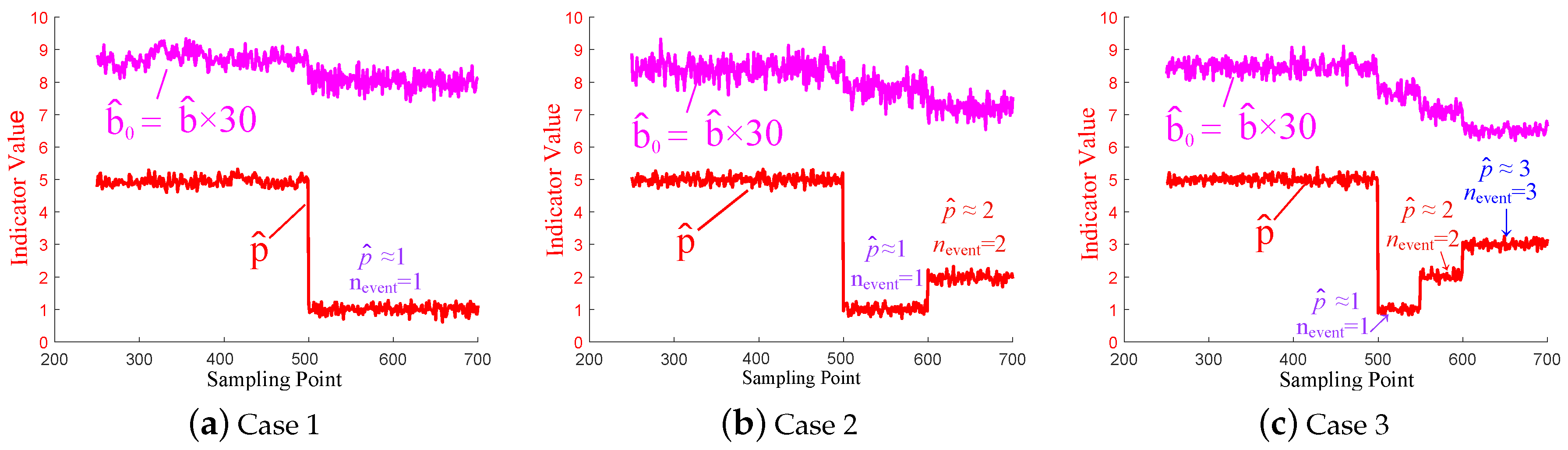
In this set of cases, the simulated data contains 118 voltage measurements with 700 sampling points, respectively. The size of the moving split-window is set as , i.e., . Then, Equation (4) is used in each split-window to estimate the parameters p and b as and : the for the number of the constituent components in a multiple event, and the for the autocorrelation structure of the residuals. The idea behind this is as follows. First, raw voltage magnitude data in each split-window is normalized using Equation (2). Then, we keep subtracting different numbers of factors from the normalized voltage magnitude data using Equation (5) until the residuals become close to the autoregressive model with autoregressive rate b as we calculate in Equation (8). The Jensen-Shannon divergence in Equation (11) is utilized to measure how “close” the two residual spectral distributions are close to each other. The optimal parameter set is finally obtained once the Jensen-Shannon divergence is minimized. Three cases are designed in this part to validate the proposed approach. In Section 4.1.1, Section 4.1.2 and Section 4.1.3, we set different numbers of constituent components in a multiple event, and the corresponding results are shown in Figure 2a–c. The experiments are repeated for 20 times and the results are averaged. We need to point out that the estimation of p and b begins at = 250 due to the length of the split-window. We amplify the value of for thirty times to make it obvious in Figure 2, i.e., .
4.1.1. Case 1—A Single Event
In Case 1, a single event, i.e., a short-circuit fault is set at Bus 64, which is shown in Table 2.
Figure 2a shows that:
- During the sampling time (250 = 1 (the beginning of the signal) + 250 (length of the split-window) − 1). and remain steady.
- At = 500, starts to decline to around 1. Also, declines slightly.
Actually, as can be seen from Table 2: no events occur in the system when keeps steady. Right at = 500, a short-circuit fault happens at Bus 64. Therefore, we can conduct the single event detection with the proposed approach. Moreover, in this case, for the split-window to , there exists a single event (a short-circuit fault at Bus 64 at = 500) and 1 factor, i.e., 1 event, .
4.1.2. Case 2—A Multiple Event with Two Constituent Components
In this case, a multiple event is set with two constituent components. One is a short-circuit fault at Bus 64, and the other is a disconnection fault at the line connected by Bus 23 and Bus 24, which is shown in Table 3.
Figure 2b shows that:
- During the sampling time , and remain steady, which is consistent with Table 3: no events occur.
- At = 500, starts to decline and then keeps around 1 till = 599. For the split-window to , there exists a single event (the short-circuit fault at Bus 64 at = 500) and 1 factor, i.e., 1 event, .
- At = 600, starts to raise and then keeps around 2. For the split-window to , there exist two constituent components (a short-circuit fault at Bus 64 at = 500 and a disconnection fault at the line connected by Bus 23 and Bus 24 at = 600) and 2 factors, i.e., 2 constituent components, .
4.1.3. Case 3—A Multiple Event with Three Constituent Components
In this case, a multiple event is set with three constituent components at Bus 64, the line connected by Bus 23 and Bus 24, and Bus 107, respectively, which is shown in Table 4.
Figure 2c shows that:
- During the sampling time , and remain steady, which is consistent with Table 4: no events occur.
- At = 500, starts to decline and then keeps around 1 till = 549. For the split-window to , there exists a single event (a short-circuit fault at Bus 64 at = 500) and 1 factor, i.e., 1 event, .
- At = 550, starts to raise and then keeps around 2 till = 599. For the split-window to , there exist two constituent components (a short-circuit fault at Bus 64 at = 500 and a disconnection fault at the line connected by Bus 23 and Bus 24 at = 550) and 2 factors, i.e., 2 constituent components, .
- At = 600, raises again and then keeps around 3. For the split-window to , there exist three constituent components (a short-circuit fault at Bus 64 at = 500, a disconnection fault at the line connected by Bus 23 and Bus 24 at = 550, and a generator tripping event at Bus 107 at = 600) and 3 factors, i.e., 3 constituent components, .
4.1.4. More Discussions of
The results of Section 4.1.1, Section 4.1.2 and Section 4.1.3 are summarized in Table 5. Based on the three cases, we can deduce that the estimated value of factors () is equal to the number of constituent components in a multiple event ().
To validate the above conclusion, we explore the empirical spectral distribution (ESD) of the covariance matrix of in Case 3. The ESD typically exhibits two aspects: a bulk and several spikes (i.e., the deviating eigenvalues). The bulk arises from noise or normal fluctuations, while the spikes are caused by faults.
Figure 3 shows that:
- At = 400, no spikes (factors) are observed. It is noted that remains almost at 5 in Figure 2c when no events occur. The most likely explanation is that some normal fluctuations of active load create several weak factors. Our approach is sensitive to weak factors under normal operating conditions. However, this phenomenon does not interfere with the judgment of the number of constituent components in a multiple event, because the number of factors is stable under normal conditions, whereas when a multiple event occurs, the change of the number of factors has a regularity.
- At = 520, one spike (factor) is observed. It is caused by the single event in the window, which is consistent with the results in Table 5.
- At = 570, two spikes (factors) are observed. They are caused by the two constituent components of a multiple event in the window.
- At = 620, three spikes (factors) are observed. They are caused by the three constituent components in the multiple event.
Note that is a spatial indicator that maps the events occurring in the system.
4.1.5. More Discussions of
In Figure 3, we can see that the estimations of and are simultaneous and interdependent. The deviating eigenvalues are factors, whose number is estimated by the indicator , whereas the region of the bulk is closely related to . In other words, derives from the signal subspace, denoting the number of signals or events, whereas derives from the noise subspace, denoting the autocorrelation rate of residuals. The number of factors can be determined only if the bulk is well fitted by the theoretical autoregressive model with parameter .
For the PMU data structure, reveals the correlation (cross-correlation) in space, and meanwhile, tracks that in time (autocorrelation). Although the number of constituent components within a multiple event is contained in the spatial information, we can see that the parameter can also reflect the status of the system based on the results in the above results. Every time a constituent component of the multiple event occurs, changes together with and can act as a temporal indicator to assist judgment.
4.2. Case Study with Real Data
In this section, we evaluate the proposed algorithm with real 34-PMU data. In the following experiment, the real power flow data of a multiple event happened in the China power grids in 2013 is utilized as the raw data for analysis. The PMU number, the sampling rate and the total sampling time are 34, 50 Hz and 284 s, respectively. The multiple event happened from 65.4 s to 73.3 s. Figure 4a,b depict the three-dimensional power flow data under normal conditions and in the case of multiple events. It can be seen that the power flow is relatively steady in the normal state whereas changes irregularly when the multiple event occurs.
In this experiment, we use a window of size (i.e., ) and move it at each sampling point. In each split-window, we estimate the number of factors and the autoregressive rate of residuals of the power flow data as the synthetic voltage magnitude data we deal with in Section 4.1. Near the occurrence of the multiple event, and are estimated, and the indicators are shown in Figure 5. From the and curves, we can realize multiple event detection and analysis as follows:
- From 60.00 s to 65.38 s, the values of and remain steady, indicating that no events occur during this period. It is noted that the value of stays around 7 rather than 5 as it is in the simulated data. One explanation is that even though noise with an SNR of 22 dB is added to the simulated data, it is still difficult to accurately mimic the fluctuations of real PMU data. The normal fluctuations of real power flow data cause some weak factors, which are detected by our algorithm.
- At 65.40 s, decreases to 1 and remains at 1 until 69.68 s. One factor is detected during this period, indicating that the first constituent component is observed in the split-window.
- From 69.70 s to 72.98 s, two factors are observed. We can speculate that at 69.70 s, the second constituent component of the multiple event occurs.
- At 73.30 s, the value of increases by 1, indicating that the third constituent component of the multiple event occurs at this moment.
As the window continues to move, the number of constituent components in the window decreases, corresponding to the decrease of value from 73.38 s to 80.98 s. In addition, as a temporal indicator to describe the autocorrelation of residuals, decreases every time a new constituent component occurs. , together with , reveals the occurrence of the multiple event.
5. Comparisons and Discussions
In this section, we compare our algorithm with two frameworks for feature selection, i.e., deep learning and PCA. We first give a review of the frameworks, and then make further analysis and comparisons.
5.1. Comparison with Deep Learning
In recent years, deep artificial neural networks have undergone a rapid development in pattern recognition and machine learning. The deep learning algorithms can automatically select features from massive data sets. The most successful form of deep learning, is supervised learning. In a typical supervised deep-learning system, hundreds of millions of labelled examples are needed to train the deep neural networks [23]. However, the real data deficiency of multiple events, especially those with labels, has greatly hindered the practical application of the supervised learning technology. In addition, the interpretability and robustness of deep learning are still being questioned [24,25,26,27]. The undesirable behaviour of deep learning has brought about concerns for AI safety [28], making it difficult to be applied to power grids with high security requirements as a result.
In contrast, the proposed high-dimensional factor model is not only “label-free”, but also has no requirements for data quantity. Moreover, our method is deeply rooted in random matrix theory and has the advantage of transparency in that our results are provable. With the aid of Equation (7), our approach is capable of dealing with spatial-temporal correlation, which is a difficulty for many common algorithms. Using powerful capabilities of free probability, Equation (7) can be analyzed in a closed form so iterative procedures can be developed to search for the two fundamental parameters, i.e., and , as defined in Equation (4).
5.2. Comparison with Principal Component Analysis (PCA)
Principal Component Analysis (PCA) is a classical method for feature selection and dimensionality reduction. It transforms highly correlated variables in the datasets into a set of simplified, uncorrelated variables that best summarize the information in the raw data. These simplified, uncorrelated variables are called Principal Components (PCs). They are ordered and preserve most of the variation that was present in the original data [29]. For more details of the PCA algorithm, readers can refer to [29].
We compare our method with PCA using moving split-windows. That is, we first choose a threshold of cumulative variance contribution rate, and then the number of PCs is determined according to the empirically determined threshold defined as follows.
where is the eigenvalue of the raw matrix after subtracting mean values within each dimension. The eigenvalues are sorted in descending order and m is their total number. is the cumulative variance contribution rate of the front k PCs and is the pre-defined threshold, . The idea behind this is simple, we keep adding the eigenvalues from large to small until the inequation (15) holds for the first time, and the k is the number of PCs we need.
Apparently, the number of PCs is closely related to the predetermined cumulative variance contribution rate . In this experiment, we choose different cumulative variance contribution rates as shown in Figure 6. Real 34-PMU data in Section 4.2 is utilized for analysis. The size of the split-window is set the same as in Section 4.2, i.e., , so that the multiple events are the same in each split-window of the two comparative experiments, and the two methods can be compared directly.
Figure 7 is a top view of Figure 6, and the number of principal components is shown by the color bar on the right side. The two figures indicate that the cumulative variance contribution rate has a significant influence on the number of principal components. The threshold, however, is set empirically in advance. Furthermore, Figure 7 shows that the number of PCs determined by PCA cannot effectively reflect the number of constituent components in the multiple event no matter what cumulative variance contribution rate we choose.
In contrast, our method can determine the number of factors without any pre-defined conditions and thus outperforms the moving split-window PCA. Both spatial and temporal information are taken into account and the respective parameters and are selected automatically to detect and analyze the multiple events.
6. Conclusions
Based on high-dimensional factor models, this paper proposes a data-driven method for multiple event detection and analysis.Jointly considering both spatial and temporal correlation, this approach is able to reveal (or even decompose) a multiple event: its constituent components and their respective details, e.g., occurring timings. This joint consideration is made possible by the recent advance in random matrix theory-based statistical methods. In particular, following [17], we model the joint correlation using Equation (7). This model is very difficult to solve analytically. Using free random variables, the analytical solution is possible. Our paper exploits this mathematical trick.
The proposed method is purely data-driven, requiring no prior knowledge of the network topology or parameters, which enables it to adapt to topology changes. Both simulated data and real PMU data is used to verify the effectiveness of the algorithm. In the future work, more extensions are possible. For example, more general modeling for noise can be employed. If we consider the auto regressive and moving average model ARMA(1,1) process, we have up to 6-th order polynomial equations [20].
Author Contributions
Conceptualization, R.C.Q.; methodology, Z.L.; software, F.Y.; validation, H.Y.; formal analysis, F.Y.; resources, R.C.Q.; writing—original draft preparation, Y.F.; writing—review and editing, X.H.; visualization, F.Y.; supervision, R.C.Q.; project administration, R.C.Q.; funding acquisition, R.C.Q.
Funding
This work is supported by the National Key R&D Program of China under Grant 2018YFF0214705 and N.S.F of China under Grant No. 61571296.
Conflicts of Interest
The authors declare no conflict of interest.
Appendix A. Key Concepts and Derivation Details
We summarize the key concepts and derivation details of free random variable techniques that we employ to derive in Section 3.2. First, consider the relationship between the Green’s Function () and the spectral density ().
Definition A1.
The Green’s Function (or Stieltjes Transform).
where , , is the spectral density of the random Hermitian matrix and is defined as , where denote the N eigenvalues of .
can be reconstructed from the imaginary part of the Green’s Function .
Then, we explore the relationship between the Green’s Function and the Moment Generating Function.
Definition A2.
Moment.
where is the n-th moment of .
Definition A3.
Moment Generating Function.
Therefore, the relationship between and is
The N-transform is the inverse transform of the Moment Generation Transform.
Definition A4.
N-transform.
Now, recall the residual defined in Equation (7). Its covariance matrix can be expressed as follows.
The N-transform of can be derived as
where free random variable (FRV) multiplication law and the cyclic property of trace are used. Note that .
Using the Moment Generating Function and its inverse relation to N-transform, we can obtain
For the AR(1) process we assume in Section 3.2, the cross-correlation matrix is . Then, . Therefore, Equation (A10) can be written as
Then we need to find the Moment Generation Function of . Recall that the auto-covariance matrix of AR(1) process can be written as in Section 3.2. Using its Fourier-transform, we can derive as
Therefore, we can obtain Equation (8).
References
- Dagle, J.E. Data management issues associated with the August 14, 2003 blackout investigation. In Proceedings of the Power Engineering Society General Meeting, Denver, CO, USA, 6–10 June 2004; Volume 2, pp. 1680–1684. [Google Scholar]
- Lai, L.L.; Zhang, H.T.; Lai, C.S.; Xu, F.Y.; Mishra, S. Investigation on July 2012 Indian blackout. In Proceedings of the International Conference on Machine Learning and Cybernetics, Lanzhou, China, 13–16 July 2014; pp. 92–97. [Google Scholar]
- Roman, R.C.; Precup, R.E.; David, R.C. Second order intelligent proportional-integral fuzzy control of twin rotor aerodynamic systems. Proc. Comput. Sci. 2018, 139, 372–380. [Google Scholar] [CrossRef]
- Han, J.; Wang, H.; Jiao, G.; Cui, L.; Wang, Y. Research on active disturbance rejection control technology of electromechanical actuators. Electronics 2018, 7, 174. [Google Scholar] [CrossRef]
- Rafferty, M.; Liu, X.; Laverty, D.M.; Mcloone, S. Real-time multiple event detection and classification using moving window PCA. IEEE Trans. Smart Grid 2016, 7, 2537–2548. [Google Scholar] [CrossRef]
- Bykhovsky, A.; Chow, J.H. Power system disturbance identification from recorded dynamic data at the Northfield substation. Int. J. Electr. Power Energy Syst. 2003, 25, 787–795. [Google Scholar] [CrossRef]
- Wang, W.; He, L.; Markham, P.; Qi, H. Detection, recognition, and localization of multiple attacks through event unmixing. In Proceedings of the IEEE International Conference on Smart Grid Communications, Vancouver, BC, Canada, 21–24 October 2013; pp. 73–78. [Google Scholar]
- Song, Y.; Wang, W.; Zhang, Z.; Qi, H.; Liu, Y. Multiple event detection and recognition for large-scale power systems through cluster-based sparse coding. IEEE Trans. Power Syst. 2017, 32, 4199–4210. [Google Scholar] [CrossRef]
- Huang, Z.; Wang, C.; Ruj, S.; Stojmenovic, M.; Nayak, A. Modeling cascading failures in smart power grid using interdependent complex networks and percolation theory. In Proceedings of the Industrial Electronics and Applications, Melbourne, VIC, Australia, 19–21 June 2013; pp. 1023–1028. [Google Scholar]
- Soltan, S.; Mazauric, D.; Zussman, G. Cascading failures in power grids: analysis and algorithms. In Proceedings of the 5th International Conference on Future Energy Systems, Cambridge, UK, 11–13 June 2014; pp. 195–206. [Google Scholar]
- He, X.; Ai, Q.; Qiu, R.C.; Huang, W.; Piao, L.; Liu, H. A big data architecture design for smart grids based on random matrix theory. IEEE Trans. Smart Grid 2017, 8, 674–686. [Google Scholar] [CrossRef]
- Chu, L.; Qiu, R.C.; He, X.; Ling, Z.; Liu, Y. Massive streaming PMU data modeling and analytics in smart grid state evaluation based on multiple high-dimensional covariance tests. IEEE Trans. Big Data 2016, 4, 55–64. [Google Scholar] [CrossRef]
- He, X.; Qiu, R.C.; Ai, Q.; Chu, L.; Xu, X.; Ling, Z. Designing for situation awareness of future power grids: An indicator system based on linear eigenvalue statistics of large random matrices. IEEE Access 2016, 4, 3557–3568. [Google Scholar] [CrossRef]
- Qiu, R.C.; Antonik, P. Smart Grid and Big Data: Theory and Practice; Wiley: Hoboken, NJ, USA, 2017. [Google Scholar]
- Chakhchoukh, Y.; Vittal, V.; Heydt, G.T. PMU based state estimation by integrating correlation. IEEE Trans. Power Syst. 2014, 29, 617–626. [Google Scholar] [CrossRef]
- Hassanzadeh, M.; Evrenosoğlu, C.Y.; Mili, L. A short-term nodal voltage phasor forecasting method using temporal and spatial correlation. IEEE Trans. Power Syst. 2016, 31, 3881–3890. [Google Scholar] [CrossRef]
- Yeo, J.; Papanicolaou, G. Random matrix approach to estimation of high-dimensional factor models. arXiv, 2016; arXiv:1611.05571. [Google Scholar]
- Forni, M.; Giovannelli, A.; Lippi, M.; Soccorsi, S. Dynamic factor model with infinite-dimensional factor space: Forecasting. J. Appl. Econ. 2018, 33, 625–642. [Google Scholar] [CrossRef] [Green Version]
- Sun, Z.; Liu, X.; Wang, L. A hybrid segmentation method for multivariate time series based on the dynamic factor model. Stoch. Environ. Res. Risk Assess. 2017, 31, 1291–1304. [Google Scholar] [CrossRef]
- Burda, Z.; Jarosz, A.; Nowak, M.A.; Snarska, M. A random matrix approach to VARMA processes. New J. Phys. 2010, 12, 075036. [Google Scholar] [CrossRef] [Green Version]
- Lixin, Z. Spectral Analysis of Large Dimentional Random Matrices. Ph.D. Thesis, National University of Singapore, Singapore, 2007. [Google Scholar]
- Zimmerman, R.D.; Murillo-Sánchez, C.E.; Thomas, R.J. MATPOWER: Steady-state operations, planning, and analysis tools for power systems research and education. IEEE Trans. Power Syst. 2011, 26, 12–19. [Google Scholar] [CrossRef]
- LeCun, Y.; Bengio, Y.; Hinton, G. Deep learning. Nature 2015, 521, 436. [Google Scholar] [CrossRef] [PubMed]
- Dumitru, M.A.K.R.M.; Pieter, E.B.K.S.D.; Kindermans, J.; Schütt, K.T. Learning how to explain neural networks: Patternnet and patternattribution. In Proceedings of the International Conference on Learning Representations, Vancouver, BC, Canada, 30 April–3 May 2018. [Google Scholar]
- Ribeiro, M.T.; Singh, S.; Guestrin, C. Why should i trust you? Explaining the predictions of any classifier. In Proceedings of the 22nd ACM SIGKDD International Conference on Knowledge Discovery and Data Mining, San Francisco, CA, USA, 13–17 August 2016; pp. 1135–1144. [Google Scholar]
- Lee, K.; Lee, H.; Lee, K.; Shin, J. Training confidence-calibrated classifiers for detecting out-of-distribution samples. arXiv, 2017; arXiv:1711.09325. [Google Scholar]
- Liang, S.; Li, Y.; Srikant, R. Enhancing the reliability of out-of-distribution image detection in neural networks. arXiv, 2017; arXiv:1706.02690. [Google Scholar]
- Amodei, D.; Olah, C.; Steinhardt, J.; Christiano, P.; Schulman, J.; Mané, D. Concrete problems in AI safety. arXiv, 2016; arXiv:1606.06565. [Google Scholar]
- Jolliffe, I. Principal Component Analysis; Springer: Berlin, Germany, 2011. [Google Scholar]
Figure 1.
Topology of the standard IEEE 118-bus system.

Figure 2.
Case Study with Simulated Data. The estimated number of constituent components in a multiple event, i.e., , is equal to the actual number of constituent components, i.e., nevent that we assume in a multiple event.
Figure 2.
Case Study with Simulated Data. The estimated number of constituent components in a multiple event, i.e., , is equal to the actual number of constituent components, i.e., nevent that we assume in a multiple event.

Figure 3.
The ESD of the covariance matrix of at different sampling points in Case 3. The bulk can be fitted well by our built model with . The numbers of spikes are different when different numbers of constituent components occurring within a multiple event, which is consistent with the results in Table 5.

Figure 4.
The real 34-PMU power flow data. (a) The real 34-PMU power flow data under normal conditions; (b) The real 34-PMU power flow data when the multiple event occurs.
Figure 4.
The real 34-PMU power flow data. (a) The real 34-PMU power flow data under normal conditions; (b) The real 34-PMU power flow data when the multiple event occurs.

Figure 5.
Indicators of the real 34-PMU power flow data around the occurrence of the multiple event.
Figure 5.
Indicators of the real 34-PMU power flow data around the occurrence of the multiple event.

Figure 6.
The number of principal components (PCs) of the real 34-PMU power flow data when different cumulative variance contribution rates are selected under the framework of PCA.
Figure 6.
The number of principal components (PCs) of the real 34-PMU power flow data when different cumulative variance contribution rates are selected under the framework of PCA.

Figure 7.
A top view of Figure 6. The number of principal components is shown by the color bar on the right side of the figure.
Figure 7.
A top view of Figure 6. The number of principal components is shown by the color bar on the right side of the figure.


Table 1.
Steps of calculating .
| (1) Calculate : each row of which is the j-th principal component of ; denote as: . |
| (2) Calculate least squares regression of on : . |
| (3) Calculate the p-level residual: . |
| (4) Calculate the covariance matrix of the p-level residual: . |
| (5) Calculate the empirical spectral distribution of . |
Table 2.
A single event assumed in Case 1.
| Bus | Sampling Time | Assumed Events |
|---|---|---|
| 64 | A short-circuit fault |
Table 3.
A multiple event with two constituent components assumed in Case 2.
| Bus | Sampling Time | Assumed Events |
|---|---|---|
| 64 | A short-circuit fault | |
| 23, 24 | A disconnection fault at the line connected by Bus 23 and Bus 24 |
Table 4.
A multiple event with three constituent components assumed in Case 3.
| Bus | Sampling Time | Assumed Events |
|---|---|---|
| 64 | A short-circuit fault | |
| 23, 24 | A disconnection fault at the line connected by Bus 23 and Bus 24 | |
| 107 | A generator tripping event |
Table 5.
Relationship between the number of constituent components in a multiple event () and the number of factors ().
Table 5.
Relationship between the number of constituent components in a multiple event () and the number of factors ().
| Case | Split-Window | ||
|---|---|---|---|
| 1 | 1 | 1 | |
| 2 | 1 | 1 | |
| 2 | 2 | 2 | |
| 3 | 1 | 1 | |
| 3 | 2 | 2 | |
| 3 | 3 | 3 |
© 2019 by the authors. Licensee MDPI, Basel, Switzerland. This article is an open access article distributed under the terms and conditions of the Creative Commons Attribution (CC BY) license (http://creativecommons.org/licenses/by/4.0/).
Share and Cite
MDPI and ACS Style
Yang, F.; Qiu, R.C.; Ling, Z.; He, X.; Yang, H. Detection and Analysis of Multiple Events Based on High-Dimensional Factor Models in Power Grid. Energies 2019, 12, 1360. https://0-doi-org.brum.beds.ac.uk/10.3390/en12071360
AMA Style
Yang F, Qiu RC, Ling Z, He X, Yang H. Detection and Analysis of Multiple Events Based on High-Dimensional Factor Models in Power Grid. Energies. 2019; 12(7):1360. https://0-doi-org.brum.beds.ac.uk/10.3390/en12071360
Chicago/Turabian StyleYang, Fan, Robert C. Qiu, Zenan Ling, Xing He, and Haosen Yang. 2019. "Detection and Analysis of Multiple Events Based on High-Dimensional Factor Models in Power Grid" Energies 12, no. 7: 1360. https://0-doi-org.brum.beds.ac.uk/10.3390/en12071360
Note that from the first issue of 2016, this journal uses article numbers instead of page numbers. See further details here.