Are Exports More Responsive to Clean or Dirty Energy? The Case of Vietnam’s Exports to 54 Countries

Abstract

In this paper we examine the influence of clean (hydropower) or dirty (fossil fuel generated) energy on bilateral exports. We focus on bilateral exports from Vietnam, a developing nation with a fast-growing economy propelled by international trade, to her top 54 trading partners over the period 1986–2010. Our key results suggest that there is a significant, positive, and stable long-term relationship between electricity and exports, with some variations across the regional panels of the trading partners and electricity sources. Trading partners of Vietnam are sensitive to how electricity is generated. For trading partners from regions excluding low income Asia, bilateral exports respond more to renewables than fossil fuel generated electricity, which indicates that exports are sensitive to certain qualities of energy sources, namely reliability and price competitiveness.

1. Introduction

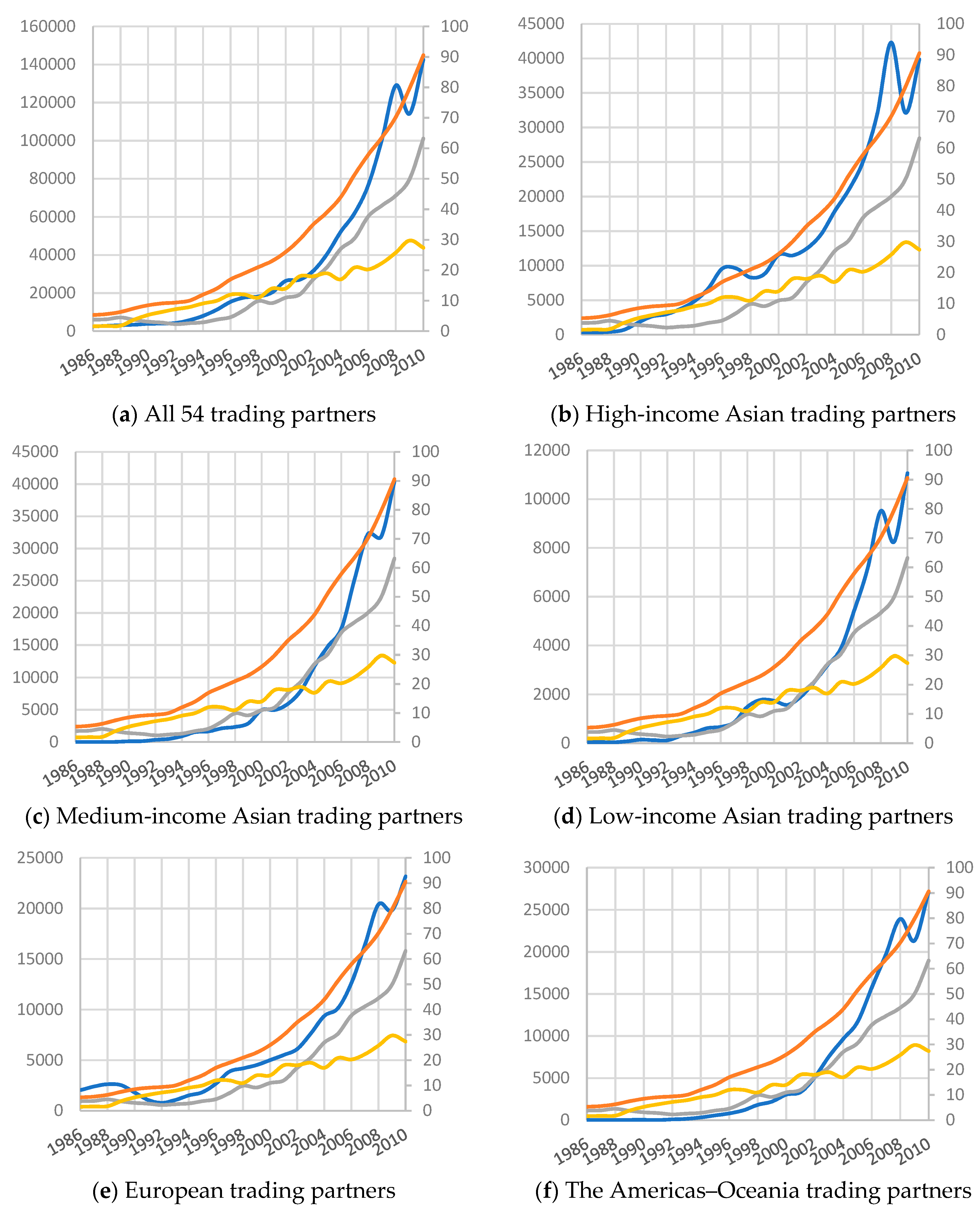
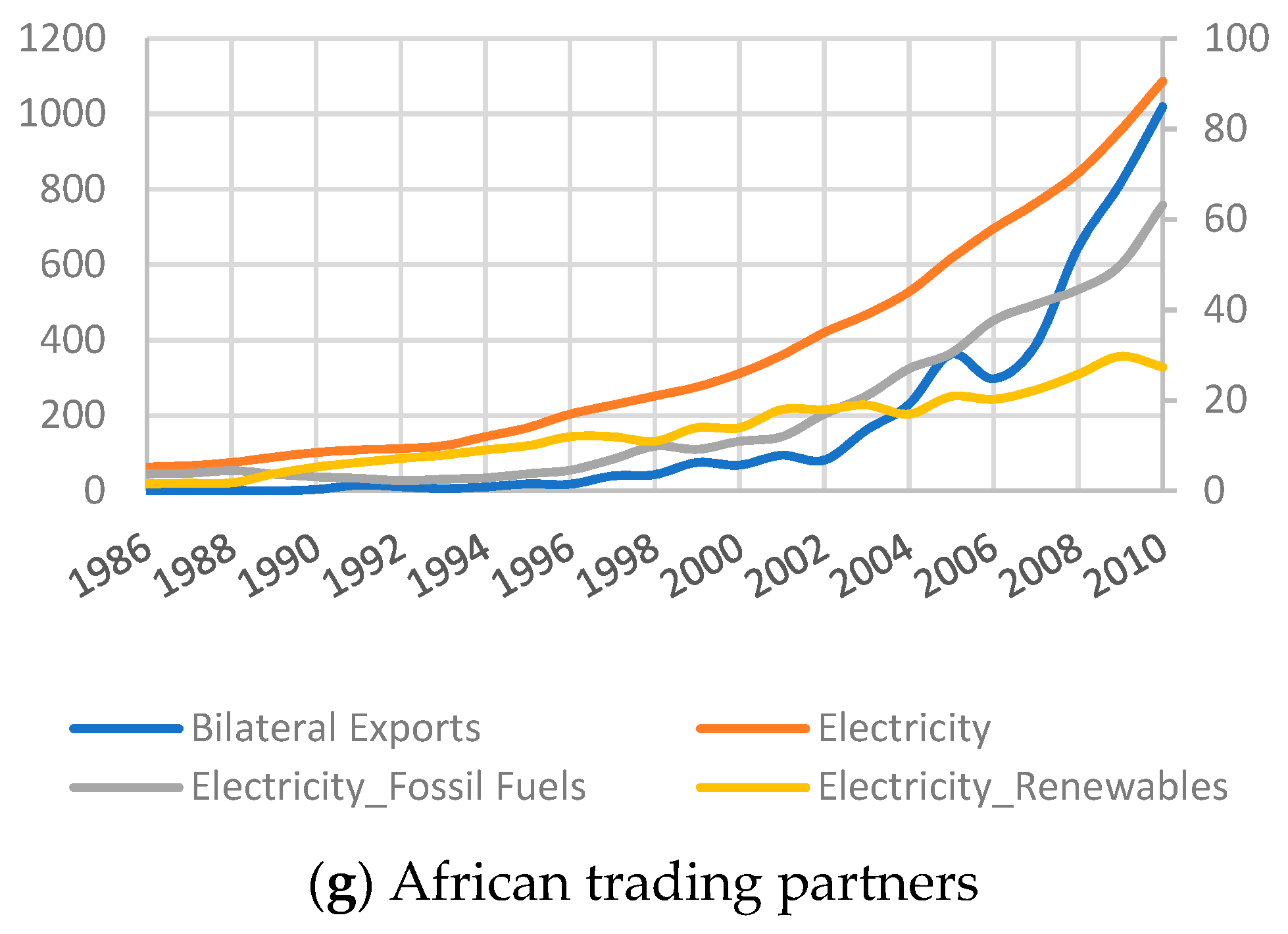
This paper investigates the role of clean and dirty energy in the export industries of Vietnam, a developing nation. For developing nations, exports have become an important driver of economic prosperity. In Vietnam, exports contributed 66.8% on average to its gross domestic product (GDP), becoming the most important driver of economic activity over the period 2000–2010 [1]. Over the period 1986–2010, Vietnamese exports accounted for 46.1% of GDP [1]. Economic prosperity has often come at the expense of environmental degradation, where energy generation has played a critical role. In many developing nations, export led growth has needed to be sustained by substantial increases in electricity generation. Often, to keep up with the ever-growing demand for energy, developing nations have resorted to using more non-renewables than renewables (see Figure 1 for the case of Vietnam). Incidentally, trade-related activities, predominantly in less industrialised countries, tend to increase a nation’s greenhouse gas (GHG) related emissions burden [2]. Hence, for developing nations, an understanding of the influence of clean versus dirty energy sources on their export industries is imperative to developing energy policies that reduce GHG emissions and promote economic growth.

The link between total energy and aggregate exports has been explored by several studies, starting with [3] (see review in Section 2). As noted above, the need to focus on the energy mix, or in this case electricity mix, has become imperative to developing modern energy policies. Energy policies across the world, including Vietnam, are still placing more reliance on fossil fuels than renewables for electricity generation. In Vietnam, fossil fuels are still the dominant source in the electricity mix, although renewable energy (almost 100% of which came from hydroelectricity) also has a strong role (

Table 1. Electricity mix in Vietnam by fossil fuels and renewables.

	Fossil Fuel	Hydro	Biomass & Waste	Wind
Panel 1: Electricity mix (billion Kwh): 1980–2014
1980–2004	6.85	7.92	0.00	0.00
2005	30.45	20.85	0.05	0.00
2006	37.68	20.20	0.07	0.00
2007	41.26	22.29	0.08	0.00
2008	44.51	25.73	0.06	0.00
2009	49.94	29.68	0.06	0.01
2010	63.21	27.28	0.06	0.05
2011	59.23	40.52	0.06	0.09
2012	60.77	52.27	0.06	0.09
2013	68.58	51.44	0.06	0.09
2014	77.29	57.96	0.06	0.09
Panel 2: Electricity mix: 2008–2014
Average quantity (billion Kwh)	60.50	40.69	0.06	0.06
Energy Mix (%)	59.72	40.17	0.06	0.06
Renewable Energy Mix (%)		99.72	0.14	0.14

Source: US Energy Information Administration.

). Electricity generation in Vietnam mainly uses fossil fuels and hydropower, contributing 55% and 45% to the electricity mix respectively (see Table 1). In comparison, when we look globally, electricity is still largely generated by non-renewables (76%), with renewables only generating 24% of the world’s electricity, of which hydropower contributes around 17% [4].

While renewables and fossil fuels are fundamentally different—the former is a clean energy source and the latter is a dirty energy source—the global trend suggests that their demand has mainly depended on energy policy, price competitiveness, reliability, and easy access. A global study by the International Renewable Energy Agency [5] showed that hydropower is more competitive than fossil fuel. The US National Hydropower Association (NHA) notes that consumers pay lower electricity costs in those American states that get the majority of their electricity from hydropower, namely Idaho, Washington, and Oregon. A US study shows that hydropower has the lowest levelized cost of electricity (accounting for the different technologies needed to collect, process and transport energy) across all major fossil fuel and renewable energy sources (see, http://www.hydro.org/why-hydro/affordable/).

However, as in the case of Vietnam, hydroelectricity is found to be unreliable. Supply outages often coincide with extreme weather conditions, such as drought. Extreme wet seasons also pose serious flooding threats for communities, particularly those in low-lying areas, close to dams that are often structurally weak. Further, while Vietnam has many hydro dams across the country, construction of new dams often generates significant opposition, based on the potential threat they pose to the local environment and livelihoods (for details, see http://factsanddetails.com/southeast-asia/Vietnam/sub5_9g/entry-3486.html).

Concern among energy users about the reliability of renewables is present in countries integrating green energy into the grid. This concern has triggered a number of researchers to examine the reliability of renewables and to develop approaches to make green energy sources more reliable (for a review on the reliability and economic evaluation of power systems with renewables, see [6]). A US study concluded that hydropower is a reliable energy source, but federal government regulations limit access to this option [7] and inhibit its development in the US. As noted by [8], fossil fuel companies have a strong influence on energy policy in the US and it is difficult to envisage full political support for renewables, unless the fossil fuel companies become politically disconnected. Notwithstanding, often when there is a political will to integrate renewables into the grid, several issues—such as those outlined for Vietnam—emerge. Academic research is making progress in identifying approaches that can ensure further reliability of renewables. In a review of the integration of renewables in Germany, [8] notes that “…a grid that derives over a quarter of its power from renewables can become a global leader in supply security—in terms of SAIDI (System Average Interruption Duration Index)—given ample reserve capacities and well-developed interconnections with neighbouring grids”. Renewables have an increasing share of the energy market in France, where the aim is to have all power supplied by the renewables sector by 2050. A study assessing the current reliability of the French power sector concludes that there is a need to install additional back-up or storage capacity to fill in the gaps in the supply of electricity [9].

At present, fossil fuels—unlike renewables—provide a steady and reliable flow of energy and cater for sudden surges in demand. In fact, as seen in Figure 1, the exponential growth in Vietnam’s exports has been largely supported by fossil fuel generated electricity. Given the differences in the two energy sources, we expect to see some differences in the sensitivity of exports to renewables and fossil fuels.

In this study we examine bilateral export relations between Vietnam and each of her top 54 trade partners. This is unlike the literature which has captured energy effects on total exports only (see a review of the literature in Section 2). Our approach allows us to test for the presence of heterogeneity in the impact of electricity (or electricity mix) on importers (organised by region) of goods made in Vietnam. We expect some variations across the regions for at least two reasons. First, the contribution to Vietnam’s exports by each region differs significantly. Over the period 1986–2010, Asia, Europe, the Americas–Oceania, and Africa contributed 59.9%, 29.7%, 10.1%, and 0.3%, respectively, to Vietnam’s total exports (see Table 4 in [10] who use the same sample as the present study). In the more recent decade (2000–2010), the average share of exports to total Vietnamese exports to these top 54 trading nations increased for Asia to 63.7%; the Americas–Oceania to 18.0% and Africa to 0.5%, and deteriorated in the case of Europe to 17.8% (see Table 4 in [10]). Second, the export mix from Vietnam varies significantly (see Table S1). Accordingly, the energy requirement of the export mix differs from one trading partner to the next. Consequently, some heterogeneity, in terms of the magnitude of the effects of energy on export by different regions, can be expected.

Foreshadowing our key results, we find strong evidence of a positive linkage between electricity and exports in the long run. This finding is robust across the panels developed according to the regions of the trading partners. Our findings suggest that the long-term electricity generated by renewables is price competitive, yet more disruptive than fossil fuel, in impacting exports.

The balance of this paper is organised in the following manner. The next section briefly reviews the strands of energy economics literature related to this study. Section 3 presents the empirical model (the gravity model), the estimation procedures and the results. Section 4 summarises the key findings and suggests policy implications.

2. Literature Review: The Link between Exports and Electricity

Two established strands of the energy economics literature, most relevant here, study the energy–trade or energy–economic growth relationship using cointegration and Granger causality approaches. Evidence of a unidirectional long-term link between electricity and trade, flowing from electricity to exports, is most common (see [3] for six middle Eastern countries; [11] for several high-, middle- and low-income countries; and [12] for Vietnam). In the short run, some studies found that exports also encourage electricity generation (see [13] for eight middle Eastern countries; [14] for Vietnam; and [15] for Portugal). Several studies showed a significant and positive relationship between trade and electricity in the short and/or long run. In other words, an increase in electricity supply leads to an increase in trade [11,13,16,17]. Some studies found significant positive effects of electricity on economic activity in the short and/or long run [12,15,18,19,20,21,22,23,24,25,26]. However, there are others that found no link between electricity and trade/output [3,27]. Some specific studies showed that economic growth in Vietnam drives energy consumption [14], while others indicated that higher energy consumption increases Vietnam’s output, stressing the importance of energy for Vietnam’s economic growth ([12,28]. Evidence of the trade impact of non-renewable energy on Vietnam, a net importer of refined petroleum, comes from [29], who suggested that oil price significantly and negatively impacted the Dong-USD exchange rate over the period 1999–2009. This implies that lower fuel prices improve the competitiveness of Vietnam’s exports. In this study we directly check whether fossil fuel generated electricity increases exports.

Between the two literature strands, research on the impact of energy mix on trade is still rather scarce, but there is ample evidence connecting economic growth with carbon emissions, which is a product of fossil fuel energy production [30,31,32,33,34]. In terms of developing nations, [35] showed that, for 30 Chinese provinces over the period 1985–2007, a 1% increase in real GDP increased carbon emissions by approximately 0.41–0.43%. In [36], the authors found a positive link between economic growth and emissions for countries in the Middle East, South Asia, East Asia, Latin America and Africa in the short- and long-term. Only in the case of Middle Eastern and South Asian countries did they find that the long-term effect of economic activity is less than the short-term, implying that carbon emissions fell with an increase in income.

Several recent studies showed that economic growth is driven by renewable energy in developing nations (see [28] for a review). We found only two studies that examine the link between renewables and trade [32,37]. In [37], the authors found no short- or long-term causality over the period 1980–2008 between renewable energy consumption and trade in 11 African countries. For a panel of 69 countries, over the period 1980–2010, [32] found that a 1% increase in renewable energy increases exports by 0.07% in the long-term.

In all, the focus of the literature is mainly on energy and trade in aggregate terms. In this study, we consider the electricity mix and bilateral trade relations in light of the preferences given to one energy source (fossil fuels) over the other (renewables) and the need for modern energy policies to be sensitive to exports.

3. Empirical Analysis

3.1. Empirical Model

To model the impact of the electricity mix on exports, we used the export gravity model. The export gravity model of Vietnam is expected to depend on various factors such as national income, per capita income, and additional elements such as distance and trade block preferences, including membership of ASEAN (Association of South East Asian Nations), APEC (Asia–Pacific Economic Co-operation) and the WTO (World Trade Organization) ([10]; also see variations of the Vietnam gravity model in [38]). We extended the gravity model [10] to account for the impact of total electricity generated and that of electricity generated by renewables and fossil fuels.

Following [39], we used a two-step procedure that separates the estimations of time variant and time invariant gravity variables. As a first step we estimated:

$$ln{X}_{ij,t}={\delta }_1+{\delta }_2\ln Electricit{y}_{it}+{\delta }_3{Z}_t+SE+{\epsilon }_{ijt}$$

(1)

where $X_{ijt}$ is export flow from Vietnam, $i$, to j trading partner at time point over the period 1986–2010. $Electricit{y}_{it}$ is either total electricity, fossil fuel (FOSSIL) or renewables (or hydro) (RENEW) generated electricity in Vietnam. Consistent with the literature, we expected to see positive effects of energy on exports. $Z_t$ captures the key determinants of exports under the trade gravity model, namely, income (Y), exchange rate (ERN), trade openness for Vietnam (VNTRADE) and Vietnam’s trading partners (PTRADE). Following previous studies, income (Y) of country $i$ or $j$ is represented as: product of GDP ($Y)$; product of GDP per capita ($PY)$; and the difference between Vietnam’s and a trading partner’s GDP per capita ($DPY).$ Given strong correlations between these three income variables (see Table S2, each of these income variables was captured into the equations one at a time. This means that we estimated three versions (a-c) of equation 1, with Y, PY, DPY captured, respectively, in models (a-c). In terms of the expected impact of the income factors, the product of GDPs (Y) captures a nation’s economic size, which should positively influence trade. This means that an increase in the size of an economy should see an increase in trade. Similarly, the product of Vietnam’s per capita GDP and trading partner j’s per capita GDP (PY) captures the level of economic development that should encourage the export flow from Vietnam. The impact of the difference of per capita incomes (DPY) depicts the difference in endowment and its impact on trade can be explained by two trade theories. Heckscher–Ohlin (H–O) theory calls for a positive impact of difference in endowment on trade, emphasising that trade volume increases as factor endowments between the countries diverge. In contrast, [40]’s hypothesis implies a negative effect of the gap in endowment, suggesting that two nations will trade more if their factor endowments are similar.

$ER{N}_{ij,t}$ is the exchange rate between Vietnam (i) and trading partner (j) at time t. Depreciation of the exchange rate (here, the Vietnamese Dong in terms of the trading partner currency) makes domestic exports relatively more competitive; hence the exchange rate effect on trade is expected to be positive. $VNTRAD{E}_{it}$ and $PTRAD{E}_{jt}$, respectively, capture trade openness of Vietnam and trading partners (js) measured as a ratio of total trade to GDP at time t. Export volume is likely to grow as Vietnam or her trading partners become more open to the world market; as a result, VNTRADE and PTRADE are expected to exert positive effects on bilateral exports.

Equation (1) is a representation of long-term models of interest to this study. This equation also forms the basis for our cointegration test for the prevalence of a stable long-term relationship between the variables. Equation (1) is estimated using the fixed effect method, allowing us to extract the specific country effects (SE), which are used to estimate the effect of the time invariant variables as part of the second step:

$$SE= {\delta }_1+{\delta }_{2}lnDis{t}_{ij}+{\delta }_3{D}_{ASEAN}+{\delta }_4{D}_{APEC}+{\delta }_5{D}_{WTO}+{ϵ}_{ijt}$$

(2)

where the specific country effects (SE) are from model (1); and DIST_ij (in natural logs form) indicates the geographic distance between Vietnam (country i) and country j. Dummies indicate whether Vietnam, i, and a trading partner, j, are in the same trading or regional blocks (ASEAN, APEC, and WTO), where the dummies are respectively D_ASEAN; D_APEC; and D_WTO, in which the values of these dummies take 1 if Vietnam and a trading partner in the dataset are in the same trade group, or take 0 otherwise.

Preferential trade agreements create favorable trading conditions for member countries; as a result, dummies for ASEAN, APEC, and WTO membership are expected to induce positive impacts on export flows. Distance between Vietnam and a trading partner inflates the cost of the transport of traded commodities; therefore, this link should bear a negative sign. Common language or common borders, which are readily used in other studies, are not captured in model (2). A common language between Vietnam and the 54 trade partners does not exist. Only three of her Asian trade partners share a border with Vietnam.

3.2. Data

To estimate the above models, annual data over the period 1986–2010 were covered for Vietnam and her top 54 trading partners. Two different sets of data were applied. The first set comprises data relating to Vietnam’s total electricity generation, and electricity generated using fossil fuels and renewables (Table 1). These time series data were sourced from the Energy Information Administration agency of the US government (see

Table 2. Variables and their definition and sources.

Variables	Definition	Sources
$i$	Home country—Vietnam
$j$	Trading partner countries
$t$	Time point
ELEC	Total electricity generated in Vietnam	US Energy Information Administration: http://www.eia.gov
FOSSIL	Total electricity of Vietnam generated by fossil fuels	US Energy Information Administration: http://www.eia.gov
RENEW	Total electricity of Vietnam generated by renewables	US Energy Information Administration: http://www.eia.gov
X	Total bilateral trade value	IMF—Direction of Trade
Y	Income variable = GDPi × GDPj	World Bank Database, GSO, Author’s calculation
PY	Per capita GDP = Per capita GDPi × Per capital GDPj	World Bank Database, GSO, Author’s calculation
DPY	Different per capita GDP = Per capita GDPi − Per capita GDPj	World Bank Database, GSO, Author’s calculation
ERN	Nominal Exchange rate of Vietnamese currency against trading partners’	IMF and Author’s calculation
VNTRADE	The openness level of Vietnam measured by the ratio of total trade to GDP	IMF and Author’s calculation
PTRADE	The openness level of trading partner j measured by the ratio of total trade to GDP	IMF and Author’s calculation
DIST	Distance between Vietnam and country j	www.cepii.fr/francegreapgh/bdd/distances.pdf
DASEAN; DAPEC; DWTO	Dummies for trade group membership, in which the values of these dummies take 1 if Vietnam and a trading partner in the dataset are in the same trade group/s (ASEAN, APEC, and WTO), or take 0 otherwise.	Author’s calculation

, rows 4–6).

The second set comprises export data of Vietnam to her 54 (main) trading partners and their determinants other than electricity. We adopted the same sample and independent variable series from the gravity bilateral trade of goods study by [10], although the present study only captures bilateral exports of goods, not exports plus imports of goods. These 54 trading partners shared approximately 96 percent of total Vietnamese exports between 1995 and 2009 (General Statistic Organization of Vietnam; accessed from: www.gso.org.vn). Exports from Vietnam to specific trading partners, income-sourced variables, and other important gravity variables were drawn from the IMF International Financial Statistics and Direction of Trade Statistics; the World Bank Database; WTO information, the French Research Centre in International Economics (CEPII), and the General Statistics Office of Vietnam (GSO). All the variables are defined in Table 2.

The data is grouped by region. The regional panels are developed based on the United Nations Classification. These include Europe (SMEUROPE) with 22 countries; Africa (SMAFRICA) with four countries; and the Americas and Oceania (SMAMERICA) with 10 countries. With only two trading partners, Australia and New Zealand, representing the Oceania region, we incorporated these into the Americas group.

Given the diversity by income within the Asian group, we split Asia into three smaller groups: high-income, with a per capita GDP equal or higher than US $12,476 (SMASIAH); medium-income, with a per capita GDP of between US $1400 and US $4035 (SMASIAM); and the low-income Asian group, with a per capita GDP lower than US $1400 (SMASIAL). These divisions are based on the World Bank income classification.

This grouping scheme was utilised when conducting panel analysis. In total we developed seven panels: SMEUROPE; SMAFRICA; SMAMERICA; SMASIAH; SMASIAM; and SMASIAL, as well as the full sample of the 54 trading partners. The specific countries in each group are listed in

Table 3. Trading partner groupings by geographical classifications.

Geographical Groups `	Group Names	Member Countries	Definitions
Asia	SMASIAH High income Asia	Hong Kong, Israel, Japan, Korea Republic, Saudi Arabia, Singapore, United Arab Emirates	Asian countries with a high income level, with a per capita Gross Domestic Product (GDP) equal to or higher than US $12,476 #
	SMASIAM Middle income Asia	China, Iran, Malaysia, Thailand, Turkey	Asian countries with a middle income level, with a per capita GDP over US$ 1400 and under US $4035 #
	SMASIAL Low income Asia	India, Indonesia, Lao PDR, Pakistan, Philippines	Asian countries with a low income level and a per capita GDP lower US $1400 #
Europe	SMEUROPE	Austria, Belgium, Bulgaria, Czech Republic, Denmark, Finland, France, Germany, Greece, Hungary, Ireland, Italy, Netherlands, Norway, Poland, Portugal, Romania, Russian Federation, Spain, Sweden, Switzerland, UK
Africa	SMAFRICA	Algeria, Egypt Arab Republic, Nigeria, South Africa
The Americas and Oceania	SMAMERICA	Argentina, Australia, Brazil, Canada, Chile, Cuba, Mexico, New Zealand, Panama, USA

Notes: ` Country sample division by geographical location (based on United Nations Classification). ^# Country sample division by income level (Classification of World Bank)).

.

3.3. Preliminary Analysis

Tables S3 and S4 provide selected descriptive statistics on the dataset comprising the export gravity factors other than electricity. Table S3 describes the dependent variable, exports, by full sample and regional groups. Over the period 1986–2010, total Vietnamese exports to regions is, on average, highest for the high-income Asian (SMASIAH) countries, followed by the middle-income Asian (SMASIAM), the Americas–Oceania (SMAMERICA), low-income Asian (SMASIAL), European ((SMEUROPE), and African (SMAFRICA) regions.

Table S4 presents the descriptive statistics on the independent variables other than electricity. It reports the size of the economy (Y), the standard of living (PY), or difference in endowment (DPY). The Americas are ahead of Europe in terms of average size of economy, but the Americas–Oceania are behind European countries, as a group, in terms of standard of living. The difference in endowment is, on average, greater between European countries and Vietnam compared to the Americas–Oceania and Vietnam. Distance is, on average, furthest between Vietnam and the Americas group, followed by Africa and the European group. Trade openness, measured as the sum of exports and imports as a percentage of GDP, averaged 100% and 80%, respectively, for Vietnam and the full sample of trading partners. In the Asian region, Vietnam is less open to trade only to the high income Asian countries (149%).

3.3.1. Unit Root Tests

The panel unit root tests, namely, Im, Pesaran, Shin, IPS, [41]; Levin, Lau, Chu, LLC, [42]; and Fisher-type test [43] were applied to examine the time series properties of the dependent and independent variables in the models. These tests have the common null hypothesis of unit root and are conducted with an intercept and a trend.

For a panel series, $y_{it}$, which has a time dimension, t, (t = 1,…..,T) and individuals, i, (i = 1,……., N), its data generation process takes the following form:

$$\Delta y_{it}= {\beta }_{ai}+{\beta }_{bi}t + \theta y_{it-1}+ {ϵ}_{it }$$

(3)

The error ${ϵ}_{it}$ is identically independently distributed across individuals in the panel. It follows the moving average (MA) process with the form ${ϵ}_{it}= \sum _{h=1}^{\infty }{\phi }_{ih}{\theta }_{it-h}+ {\epsilon }_{it}$. ${ϵ}_{it}$ is assumed to be a stationary moving average, MA, process. ${\beta }_{ai}$ and ${\beta }_{bi}$ are parameters for the intercept and the time trend correspondingly, which vary across individual countries.

The LLC [42] tests the null hypothesis, $H_0,$ that all individual series of the panel contain a unit root ($\theta =0)$ against the alternative hypothesis $H_1:\theta <0$, and that all individual series are stationary. The LLC test assumes independence between cross sections and homogenous autoregressive estimators for all individuals in the panel. This means that $\theta$ is assumed to be the same for all individuals. The test statistic values to evaluate the null against the alternative hypotheses are derived from the pooled estimation across individual countries. Appropriate lag orders are applied to orthogonalize residuals of the auxiliary regressions, which can be expressed as:

$$\Delta y_{it }= \theta y_{it-1}+ {\displaystyle \sum }_{K=1}^{Z_i}{\phi }_{iK}\Delta y_{it-K}+ {\beta }_{Pi}{d}_{Pt}+{ϵ}_{it}$$

(4)

In model (4), the difference of each series is regressed on 1 to $Z_i$ lags ($K=1,\dots .,Z_i)$. The deterministic elements are captured in $d_{Pt}$. There is homogeneity of the autoregressive parameter, and heterogeneity in the error variance and the serial correlation structure of the errors.

The IPS [41] test is different from the LLC test in that the IPS test allows for heterogeneity of the autoregressive parameters for each individual country. The null hypothesis of the IPS test states that there is a common unit root test present for the panel, that is $H_0: {\theta }_i=\theta =0$ for all i. This is tested against the alternative hypothesis of the IPS test as: $H_1: {\theta }_i<0, i=1,\dots ..,H;and {\theta }_i=0, i=H+1, \dots \dots ,N$. There is a subset of series $y_{it}$ that is not stationary; hence the alternative hypothesis in IPS is not as restrictive as the LLC test.

The [44] test in [43] is a combination of several unit root tests, combining the p-values from different tests. The Fisher test works with the null hypothesis that there is a unit root for all $y_i, H_0: {\theta }_i=\theta$= 0, which is tested against the alternatives: (i) $H_1: {\theta }_i=\theta$< 0; or (ii) $H_1: {\theta }_i$ < 0 for $i=1,2,\dots .K;and {\theta }_i=0 for i=K+1,\dots \dots ,N.$ The scope of the alternative hypothesis in this case is broader under the Fisher test than for the LLC and IPS tests because the coverage of alternative hypotheses in the Fisher test accounts for both the LLC and IPS approaches. In [43], the authors note that the Fisher test is preferred to the IPS test in the case of unbalanced panel data.

Results presented in

Table 4. Testing the unit root for series of electricity generated in Vietnam with different regional country groups.

	$\mathit{E}\mathit{L}\mathit{E}\mathit{C}$			$\mathit{F}\mathit{O}\mathit{S}\mathit{S}\mathit{I}\mathit{L}$			$\mathit{R}\mathit{E}\mathit{N}\mathit{E}\mathit{W}$
Methods	LLC	IPS	ADF	LLC	IPS	ADF	LLC	IPS	ADF
SMASIAH	4.894	7.249	0.029	3.321	5.536	0.272	−1.306	1.521	6.179
	1.000	1.000	1.000	1.000	1.000	1.000	0.096	0.936	0.962
SMASIAL	4.137	6.127	0.020	2.807	4.679	0.194	−1.104	1.284	4.414
	1.000	1.000	1.000	0.998	1.000	1.000	0.135	0.900	0.927
SMEUROPE	8.677	12.852	0.090	5.887	9.814	0.854	−2.316*	2.702	19.420
	1.000	1.000	1.000	1.000	1.000	1.000	0.010	0.997	1.000
SMAFRICA	3.700	5.480	0.016	2.510	4.185	0.155	−0.987	1.147	3.531
	1.000	1.000	1.000	0.994	1.000	1.000	0.162	0.874	0.897
SMAMERICA	5.850	8.664	0.041	3.969	6.616	0.388	−1.561	1.820	8.827
	1.000	1.000	1.000	1.000	1.000	1.000	0.059	0.966	0.985

This table summarises unit root test results relating to three energy variables in level form: total electricity generated in Vietnam ($ELEC$); total electricity generated in Vietnam using fossil fuels $\left(FOSSIL\right)$; and total electricity generated in Vietnam from renewables $(RENEW$). Results are presented by regional group. Three unit root tests are applied with the series, including [41,42,43].

only relate to electricity variables for the seven panels. Almost always the three tests are unable to reject the null hypothesis of a unit root, implying that the variables are I(1). Our non-tabulated results suggest that for other time-variant independent and dependent variables (exports, income, per capita income, per capita income difference, exchange rate, Vietnam’s openness, and trading partners’ openness) across different region groups, the null hypothesis of a unit root cannot be rejected by at least two of the three tests. These results are available on request from the authors.

Only in the case of the middle-income Asian group did we find that exports are stationary at level form. With evidence of non-stationarity of the variables, we proceeded with the cointegration and the VECM analyses for all panels, except SMASIAM.

3.3.2. Pairwise Granger causality test

As part of the preliminary tests, we performed the pairwise Granger causality test where we tested whether: (a) electricity Granger causes exports; and (b) exports Granger causes electricity, using the following models:

$$ln \Delta X_{ij,t}={\delta }_1+{\delta }_2{\displaystyle \sum }_{p=1}^{p}ln\Delta X_{ij,t-p}+{\delta }_2{\displaystyle \sum }_{p=1}^p\ln Electricit{y}_{it-p}+{\epsilon }_{1t}$$

(5)

$$\ln Electricit{y}_{it}={\delta }_1+{\delta }_2{\displaystyle \sum }_{q=1}^q\ln Electricit{y}_{it-q}+{\delta }_2{\displaystyle \sum }_{q=1}^{q}ln\Delta X_{ij,t-q}+{\epsilon }_{2t}$$

(6)

Models (5) and (6) were estimated for total electricity, fossil fuel generated electricity and hydroelectricity. Here $\delta s$ are the parameters to be estimated; p and q are lag length, derived using the Schwarz information criteria; and $\epsilon$ is the disturbance term. The causality test is readily carried out in the Energy (E)–Income (Y) literature. Four hypotheses are relevant here: (1) the growth hypothesis suggests causality running from E to Y; the conservation hypothesis sees Y causing E; the feedback hypothesis treats both E and Y as leading each other; and the neutrality hypothesis sees no linkage between E and Y (refer to [45] and [28] for further explanation). As exports are an important engine of economic growth, we conducted the Granger causality test under the four E–Y hypotheses. The growth hypothesis justifies our study while the conservative hypothesis would suggest that trading partners can influence Vietnam’s energy policy.

The F-statistics and p-values relating to the models for total electricity, fossil fuel generated electricity and hydroelectricity are presented in Table S5. While Vietnam’s exports to these 54 trading partners are found to be Granger caused by electricity, the results are strongly dependent on the trading partners and electricity mix. In the case of total electricity, for all panels, except for those with Asian nations, the growth hypothesis is found to prevail, which means that total electricity promotes exports. For fossil fuel generated electricity, we found that a mixture of hypotheses were satisfied, depending on the panel examined: the feedback hypothesis applies for trade with the high-income Asian, European, and full sample of trading partners; the neutral hypothesis applies for the Americas; and the growth hypothesis applies in the case of low-income Asian nations and Africa.

In the case of renewables, for Europe, we noticed a feedback effect between exports and hydroelectricity, which means that there is a bi-directional link between exports and hydroelectricity. Most panels, namely the full sample, low-income Asia, Africa and the Americas seemed to show the prevalence of the conservative hypothesis, which suggests a uni-directional link flowing from exports to hydroelectricity. In contrast, the high-income Asian trading partners panel showed a neutral effect.

Next, we examined the long-term effects of total electricity and electricity mix on exports under a multivariate setting defined by the gravity export models (Equations (1–2)). Prior to estimating the long-term models, we tested for a cointegrating link between the variables in Equation (1).

3.4. Cointegration Test

We relied on [46] to conduct the cointegration tests. We only cover the time variant factors here. This test is a residual based test that assumes homogeneity of the panel data and tests the null hypothesis of no cointegration. In our panel analysis, the several data series, namely, exports, exchange rate between Vietnam and the 54 trading partners, and income variables relating to the 54 trading partners, vary by country. Our estimation scheme accounts for some cross-sectional heterogeneity in our sample by dividing the data into trading partners’ regional panels. In the case of Asia, we noted some heterogeneity, which led us to subdivide the sample by income (see Section 3.2). While we do not claim to have accounted for all heterogeneity in the panel data we use here, we have accounted for those that are related to regional and income difference. A similar panel scheme adopted by [10] showed that the Kao test gave consistent results for the gravity trade model as did another panel based cointegration test, namely the [47,48] test that accounted for heterogeneity and homogeneity of the panel data.

The Kao test considers strict regressors that are either endogenous or exogenous. Kao estimated a Least Squares Dummy Variable (LSDV) model with variables which are integrated to order one, I(1), to evaluate the long-term relationship between the dependent and independent variables:

$$y_{i.t}= {\phi }_i+\gamma x_{i,t}+{\epsilon }_{i,t }$$

(7)

with $i=1,2,\dots .,N;and t=1,2,\dots ,T$. $Y$ is the dependent variables while $X$ comprises independent variables in model 1. For model (7), the parameter ${\phi }_i$ may vary across the bilateral relationships covered while the coefficients for regressors, $\gamma$, are common across members. To test for cointegration, Kao employed the Dickey–Fuller autoregressive model and the Augmented Dickey–Fuller autoregressive model for testing the residuals, ${\epsilon }_{i,t }$, in (7). For the existence of a long-term relationship to the system (7), ${\widehat{\epsilon }}_{i,t}$ needs to be I(0).

Table 5. Cointegration between exports and electricity—the Kao test results.

	SMAFRICA		SMAMERICA		SMEUROPE		SMASIAH		SMASIAL
	Statistic	Prob.	Statistic	Prob.	Statistic	Prob.	Statistic	Prob.	Statistic	Prob.
1. Total electricity
Model a	−1.914	0.028	−6.320	0.000	−6.789	0.000	−1.686	0.046	−3.701	0.000
Model b	−1.976	0.024	−6.339	0.000	−6.830	0.000	−1.578	0.057	−3.712	0.000
Model c	−2.214	0.013	−6.708	0.000	−7.005	0.000	−1.592	0.056	−3.575	0.000
2. Fossil fuel generated electricity
Model a	−1.857	0.032	−5.056	0.000	−5.405	0.000	−1.695	0.045	−3.963	0.000
Model b	−2.003	0.023	−5.179	0.000	−5.332	0.000	−1.429	0.077	−3.991	0.000
Model c	−2.552	0.005	−6.652	0.000	−5.563	0.000	−1.674	0.047	−3.868	0.000
3. Renewable energy generated electricity
Model a	−1.891	0.029	−5.897	0.000	−6.559	0.000	−1.824	0.034	−3.158	0.001
Model b	−1.978	0.024	−5.912	0.000	−6.405	0.000	−1.651	0.049	−3.132	0.001
Model c	−3.102	0.001	−6.526	0.000	−5.461	0.000	−2.017	0.022	−3.061	0.001

This table reports the Kao test results. The null hypothesis of no co-integration among the variables in models a–c is tested. As shown in Table S2, due to the strong correlation of the three income-sourced variables: $ln{Y}_{ijt}$, $lnP{Y}_{ijt}$, and $lnDP{Y}_{ijt}$, three separate models are introduced here:$ln{X}_{ijt}={\delta }_{1 }+ {\delta }_{2}ln{Y}_{ijt}+{\delta }_{3}lnElectricit{y}_{it}+{\delta }_{4}lnER{N}_{ijt}+{\delta }_{5}VNTRAD{E}_{it}+{\delta }_{6}lnPTRAD{E}_{jt}+ {\epsilon }_{ijt}$ (a); $ln{X}_{ijt}={\delta }_{1 }+ {\delta }_{2}lnP{Y}_{ijt}+{\delta }_{3}lnElectricit{y}_{it}+{\delta }_{4}lnER{N}_{ijt}+{\delta }_{5}VNTRAD{E}_{it}+{\delta }_{6}lnPTRAD{E}_{jt}+ {\epsilon }_{ijt}$ (b); $ln{X}_{ijt}={\delta }_{1 }+ {\delta }_{2}lnDPY{N}_{ijt}+{\delta }_{3}lnElectricit{y}_{it}+{\delta }_{4}lnER{N}_{ijt}+{\delta }_{5}VNTRAD{E}_{it}+{\delta }_{6}lnPTRAD{E}_{jt}+ {\epsilon }_{ijt}$ (c). These are estimated for electricity variables, measured as: (1) total electricity; (2) fossil fuel generated electricity; or (3) renewable energy generated electricity. This means we estimate nine models for each subsample. The numbers in bold are test statistics, and those in italics indicate the probability of rejecting the null hypothesis.

summarises the Kao test results. For all panels we rejected the null hypothesis of no cointegration at 5% or better. A stable long-term relationship between the variables described in equation (1) is indicated by the test.

3.5. Long-Term Linkages

3.5.1. Electricity and Exports

Next, we examined the long-term relationship between electricity and bilateral exports of Vietnam.

Table 6. Long-term effect of electricity generated in Vietnam on exports: Full sample.

	Model	$\mathit{l}\mathit{n}\mathit{Y}$	$\mathit{l}\mathit{n}\mathit{P}\mathit{Y}$	$\mathit{l}\mathit{n}\mathit{D}\mathit{P}\mathit{Y}$	$\mathit{l}\mathit{n}\mathit{E}\mathit{R}\mathit{N}$	$\mathit{l}\mathit{n}\mathit{E}\mathit{l}\mathit{e}\mathit{c}\mathit{t}\mathit{r}\mathit{i}\mathit{c}\mathit{i}\mathit{t}\mathit{y}$	$\mathit{V}\mathit{N}\mathit{T}\mathit{R}\mathit{A}\mathit{D}\mathit{E}$	$\mathit{P}\mathit{T}\mathit{R}\mathit{A}\mathit{D}\mathit{E}$	$\mathit{l}\mathit{n}\mathit{D}\mathit{I}\mathit{S}\mathit{T}$	$\mathit{D}\mathit{A}\mathit{S}\mathit{E}\mathit{A}\mathit{N}$	$\mathit{D}\mathit{A}\mathit{P}\mathit{E}\mathit{C}$	$\mathit{D}\mathit{W}\mathit{T}\mathit{O}$	${\mathit{R}}^2$
1	2	3	4	5	6	7	8	9	10	11	12	13	14
Total	a	0.131			0.306 ***	2.687 ***	−0.007	−0.020 ***	−1.897 ***	0.365	1.171 ***	−0.225	0.8013
		0.332			0.000	0.000	0.417	0.000	0.000	0.109	0.000	0.113
	b		0.053		0.297 ***	2.856 ***	−0.008	−0.020 ***	−1.855 ***	0.222	1.315 ***	−0.233	0.8010
			0.708		0.000	0.000	0.347	0.000	0.000	0.338	0.000	0.107
	c			−0.092	0.293 ***	2.956 ***	−0.008	−0.020 ***	−1.741 ***	0.097	1.406 ***	−0.220	0.8012
				0.293	0.000	0.000	0.358	0.000	0.000	0.692	0.000	0.151
Fossil fuel	a	0.545 **			0.407 ***	0.617 *	0.019 **	−0.019 ***	−2.179 ***	0.965 ***	0.603 ***	−0.235	0.7885
		0.014			0.000	0.045	0.012	0.000	0.000	0.000	0.000	0.083
	b		0.451		0.413 ***	0.741 **	0.020 ***	−0.019 ***	−2.187 ***	0.566 ***	1.072 ***	−0.297 **	0.7859
			0.074		0.000	0.021	0.009	0.000	0.000	0.008	0.000	0.026
	c			−0.113	0.398 ***	1.133 ***	0.021 ***	−0.019 ***	−1.803 ***	0.109	1.370 ***	−0.242	0.7817
				0.185	0.000	0.000	0.009	0.000	0.000	0.654	0.000	0.111
Renewables	a	0.701 ***			0.154	1.327 ***	0.012 **	−0.018 ***	−1.988 ***	1.046 ***	0.512 ***	−0.178	0.7970
		0.000			0.059	0.000	0.015	0.000	0.000	0.000	0.000	0.177
	b		0.679 ***		0.139	1.409 ***	0.014 ***	−0.018 ***	−2.032 ***	0.595 ***	1.080 ***	−0.264 **	0.7943
			0.000		0.098	0.000	0.005	0.000	0.000	0.003	0.000	0.033
	c			0.031	−0.045	1.554 ***	0.027 ***	−0.018 ***	−1.427 ***	−0.023	1.456 ***	−0.165	0.7790
				0.796	0.422	0.000	0.000	0.000	0.000	0.922	0.000	0.260

This table shows the long-term effects of electricity, measured as total electricity, fossil fuel generated electricity, and renewable energy generated electricity on Vietnam’s exports for the total sample of 54 trading partners. Results relating to Equation (1) are displayed in columns 3-9 and are derived from: (a)$ln{X}_{ijt}={\delta }_{1 }+SE+{\delta }_{2}ln{Y}_{ijt}+{\delta }_{3}lnElectricit{y}_{it}+{\delta }_{4}lnER{N}_{ijt}+{\delta }_{5}VNTRAD{E}_{it}+{\delta }_{6}lnPTRAD{E}_{jt}+ {\epsilon }_{ijt}$; (b)$ln{X}_{ijt}={\delta }_{1 }+ SE+{\delta }_{2}lnP{Y}_{ijt}+{\delta }_{3}lnElectricit{y}_{it}+{\delta }_{4}lnER{N}_{ijt}+{\delta }_{5}VNTRAD{E}_{it}+{\delta }_{6}lnPTRAD{E}_{jt}+ {\epsilon }_{ijt}$; or (c)$ln{X}_{ijt}={\delta }_{1 }+SE+ {\delta }_{2}lnDP{Y}_{ijt}+{\delta }_{3}lnElectricit{y}_{it}+{\delta }_{4}lnER{N}_{ijt}+{\delta }_{5}VNTRAD{E}_{it}+{\delta }_{6}lnPTRAD{E}_{jt}+ {\epsilon }_{ijt}$. The impact of time-constant variables (in columns 10-13), is estimated on the SE which captures the specific effects corresponding to Equation (1), model (a), (b) or (c). The last column is the adjusted R-squared for each model. For each panel, the numbers in bold are coefficients while those in italics are respective probabilities of rejecting the null hypotheses proposed. Fixed effect estimation is used with [49] cross-section standard errors and covariance. *, ** and *** denote level of significance at 10%, 5% and 1%.

,

Table 7. Long-term influence of total electricity generated in Vietnam on its exports: Regional groups.

	Model	$\mathit{l}\mathit{n}\mathit{Y}$	$\mathit{l}\mathit{n}\mathit{P}\mathit{Y}$	$\mathit{l}\mathit{n}\mathit{D}\mathit{P}\mathit{Y}$	$\mathit{l}\mathit{n}\mathit{E}\mathit{R}\mathit{N}$	$\mathit{l}\mathit{n}\mathit{E}\mathit{l}\mathit{e}\mathit{c}\mathit{t}\mathit{r}\mathit{i}\mathit{c}\mathit{i}\mathit{t}\mathit{y}$	$\mathit{V}\mathit{N}\mathit{T}\mathit{R}\mathit{A}\mathit{D}\mathit{E}$	$\mathit{P}\mathit{T}\mathit{R}\mathit{A}\mathit{D}\mathit{E}$	$\mathit{l}\mathit{n}\mathit{D}\mathit{I}\mathit{S}\mathit{T}$	$\mathit{D}\mathit{A}\mathit{S}\mathit{E}\mathit{A}\mathit{N}$	$\mathit{D}\mathit{A}\mathit{P}\mathit{E}\mathit{C}$	$\mathit{D}\mathit{W}\mathit{T}\mathit{O}$	${\mathit{R}}^2$
1	2	3	4	5	6	7	8	9	10	11	12	13	14
SMASIAH	a	0.513 ***			0.147 ***	0.484 *	0.015 ***	−0.014 ***	−3.749 ***	4.368***	−0.209	−0.199	0.9178
		0.000			0.011	0.089	0.001	0.000	0.000	0.000	0.388	0.441
	b		0.421 ***		0.138 **	0.772 ***	0.013 ***	−0.014 ***	−3.511 ***	3.393***	0.461 *	−0.358	0.9153
			0.005		0.023	0.012	0.004	0.000	0.000	0.000	0.077	0.196
	c			0.502	0.019	1.404 ***	0.008 *	−0.014 ***	−3.449 ***	3.728***	0.220	−0.300	0.9139
				0.115	0.769	0.000	0.097	0.000	0.000	0.000	0.369	0.252
SMASIAL	a	−0.379 *			0.197 **	2.594 ***	0.004	−0.004	0.137	0.639	1.437 ***	−0.466	0.8158
		0.091			0.019	0.000	0.608	0.721	0.510	0.133	0.004	0.248
	b		−0.374 *		0.193 **	2.482 ***	0.005	−0.005	−0.650 ***	0.711 *	1.464 ***	−0.497	0.8159
			0.095		0.025	0.000	0.602	0.698	0.001	0.064	0.001	0.172
	c			0.040	0.276 ***	1.780 ***	0.010	−0.001	−0.779 ***	0.742 *	1.166 ***	−0.459	0.8126
				0.780	0.002	0.002	0.380	0.944	0.000	0.051	0.009	0.202
SMEUROPE	a	0.097			0.433 ***	3.112 ***	−0.016	−0.027 ***	3.205 ***		1.618 ***	−0.044	0.7653
		0.581			0.000	0.000	0.195	0.000	0.000		0.001	0.824
	b		0.027		0.425 ***	3.271 ***	−0.018	−0.027 ***	3.536 ***		1.795 ***	−0.049	0.7651
			0.877		0.000	0.000	0.156	0.000	0.000		0.001	0.810
	c			−0.715 ***	0.424 ***	3.525 ***	−0.015	−0.028 ***	6.914 ***		1.229 **	−0.033	0.7704
				0.011	0.000	0.000	0.190	0.000	0.000		0.035	0.884
SMAFRICA	a	0.397			0.592 ***	3.085 ***	−0.020*	−0.009	1.772 ***			−0.488 *	0.7232
		0.274			0.009	0.000	0.095	0.617	0.001			0.059
	b		0.312		0.565 ***	3.287 ***	−0.020	−0.011	1.819 ***			−0.394 *	0.7217
			0.371		0.014	0.000 ***	0.101	0.547	0.000			0.092
	c			−0.157	0.459 ***	3.480 ***	−0.015	−0.017	1.467 ***			−0.455 **	0.7212
				0.351	0.014	0.000	0.265	0.305	0.001			0.035
SMAMERICA	a	0.801 ***			0.409 ***	3.881 ***	−0.037 **	0.010	−2.569 ***		0.361 **	−0.179	0.8145
		0.008			0.000	0.000	0.046	0.410	0.000		0.016	0.340
	b		0.750 ***		0.408 ***	4.129***	−0.037 **	0.009	−1.742 ***		0.610 ***	−0.277	0.8136
			0.012		0.000	0.000	0.046	0.443	0.000		0.001	0.227
	c			0.440	0.292 ***	5.121***	−0.043 **	0.007	−2.670 ***		0.502 ***	−0.244	0.8083
				0.063	0.006	0.000	0.045	0.532	0.000		0.004	0.267

This table displays the effect of total electricity by the regions of the trading partners: SMASIAH, SMASIAL, SMEUROPE, SMAFRICA, and SMAMERICA. Results relating to Equation (1) are derived from: (a)$ln{X}_{ijt}={\delta }_{1 }+{\delta }_{2}ln{Y}_{ijt}+{\delta }_{3}lnElectricit{y}_{it}+{\delta }_{4}lnER{N}_{ijt}+{\delta }_{5}VNTRAD{E}_{it}+{\delta }_{6}lnPTRAD{E}_{jt}+ {\epsilon }_{ijt}$; (b)$ln{X}_{ijt}={\delta }_{1 }+{\delta }_{2}lnP{Y}_{ijt}+{\delta }_{3}lnElectricit{y}_{it}+{\delta }_{4}lnER{N}_{ijt}+{\delta }_{5}VNTRAD{E}_{it}+{\delta }_{6}lnPTRAD{E}_{jt}+ {\epsilon }_{ijt}$; or (c) $ln{X}_{ijt}={\delta }_{1 }+ {\delta }_{2}lnDP{Y}_{ijt}+{\delta }_{3}lnElectricit{y}_{it}+{\delta }_{4}lnER{N}_{ijt}+{\delta }_{5}VNTRAD{E}_{it}+{\delta }_{6}lnPTRAD{E}_{jt}+ {\epsilon }_{ijt}$. These equations relate to time-variant determinants on exports and are displayed in columns 3–9. The impact of time-constant variables (in columns 10-13) is estimated on the SE which captures the specific effects from Equation (1), model (a), (b) or (c).. The adjusted R-squared for each model is reported in the last column. For each panel the numbers in bold are coefficients while those in italics are respective probabilities. Fixed effect estimation is used with [49] cross-section standard errors and covariance. *, ** and *** denote level of significance at 10%, 5% and 1%.

,

Table 8. Long-term effects of electricity generated by fossil fuels on exports: Regional groups.

	Model	$\mathit{l}\mathit{n}\mathit{Y}$	$\mathit{l}\mathit{n}\mathit{P}\mathit{Y}$	$\mathit{l}\mathit{n}\mathit{D}\mathit{P}\mathit{Y}$	$\mathit{l}\mathit{n}\mathit{E}\mathit{R}\mathit{N}$	$\mathit{l}\mathit{n}\mathit{E}\mathit{l}\mathit{e}\mathit{c}\mathit{t}\mathit{r}\mathit{i}\mathit{c}\mathit{i}\mathit{t}\mathit{y}$	$\mathit{V}\mathit{N}\mathit{T}\mathit{R}\mathit{A}\mathit{D}\mathit{E}$	$\mathit{P}\mathit{T}\mathit{R}\mathit{A}\mathit{D}\mathit{E}$	$\mathit{l}\mathit{n}\mathit{D}\mathit{I}\mathit{S}\mathit{T}$	$\mathit{D}\mathit{A}\mathit{S}\mathit{E}\mathit{A}\mathit{N}$	$\mathit{D}\mathit{A}\mathit{P}\mathit{E}\mathit{C}$	$\mathit{D}\mathit{W}\mathit{T}\mathit{O}$	${\mathit{R}}^2$
1	2	3	4	5	6	7	8	9	10	11	12	13	14
SMASIAH	a	0.627 ***			0.174 ***	0.080	0.019 ***	−0.014 ***	−3.801 ***	4.505***	−0.313	−0.174	0.9172
		0.000			0.002	0.547	0.000	0.000	0.000	0.000	0.195	0.499
	b		0.614 ***		0.190 ***	0.155	0.020 ***	−0.014 ***	−3.514 ***	3.230***	0.557 **	−0.380	0.9139
			0.000		0.001	0.287	0.000	0.000	0.000	0.000	0.033	0.170
	c			0.811 **	0.089	0.578 ***	0.018 ***	−0.014 ***	−3.451 ***	3.515***	0.343	−0.327	0.9072
				0.023	0.199	0.001	0.001	0.000	0.000	0.000	0.153	0.201
SMASIAL	a	−0.220			0.527 ***	1.421 ***	0.014 *	0.003	−0.454	1.050**	1.207 **	−0.576	0.8211
		0.237			0.000	0.000	0.064	0.770	0.066	0.037	0.039	0.227
	b		−0.268		0.518 ***	1.443 ***	0.014 *	0.003	−0.897 ***	1.090**	1.254 **	−0.598	0.8218
			0.179		0.000	0.000	0.069	0.808	0.000	0.025	0.027	0.193
	c			0.073	0.539 ***	1.223 ***	0.013 *	0.005	−0.973 ***	1.052**	1.013	−0.545	0.8199
				0.582	0.000	0.000	0.088	0.688	0.000	0.029	0.068	0.229
SMEUROPE	a	0.647 **			0.488 ***	0.423	0.020 **	−0.024 ***	0.455		0.829	−0.023	0.7423
		0.025			0.000	0.322	0.050	0.000	0.500		0.063	0.898
	b		0.546 *		0.499 ***	0.560	0.020 **	−0.024 ***	1.441		2.352 ***	−0.064	0.7386
			0.080		0.000	0.198	0.046	0.000	0.065		0.000	0.753
	c			−0.782 ***	0.505 ***	1.267 ***	0.024 ***	−0.026 ***	7.352 ***		1.377 **	−0.037	0.7366
				0.014	0.000	0.001	0.012	0.000	0.000		0.021	0.873
SMAFRICA	a	0.830			0.722 **	0.814	0.007	−0.002	1.891 ***			−0.548 *	0.6899
		0.103			0.031	0.266	0.555	0.937	0.003			0.082
	b		0.642		0.670*	0.988	0.012	−0.005	2.018 ***			−0.350	0.6810
			0.203		0.061	0.175	0.395	0.798	0.001			0.212
	c			−0.375	0.538	1.388 **	0.018	−0.017	1.548 ***			−0.528	0.6831
				0.092	0.150	0.022	0.292	0.345	0.005			0.051
SMAMERICA	a	1.189 ***			0.697 ***	1.733 ***	−0.019	0.020	−1.303 ***		0.600 ***	−0.259	0.8064
		0.004			0.000	0.000	0.199	0.080	0.001		0.011	0.383
	b		1.112 ***		0.715 ***	1.893 ***	−0.017	0.019	−0.009		0.999 ***	−0.415	0.8030
			0.010		0.000	0.000	0.256	0.091	0.983		0.000	0.175
	c			0.515 **	0.649 ***	2.649 ***	−0.017	0.019	−1.320 ***		1.023 ***	−0.442	0.7887
				0.054	0.000	0.000	0.297	0.119	0.001		0.000	0.135

This table displays the effect of total electricity generated using fossil fuel (LFOSS) by the regions of the trading partners: SMASIAH, SMASIAL, SMEUROPE, SMAFRICA, and SMAMERICA. Results relating to Equation (1) are derived from: (a)$ln{X}_{ijt}={\delta }_{1 }+{\delta }_{2}ln{Y}_{ijt}+{\delta }_{3}lnElectricit{y}_{it}+{\delta }_{4}lnER{N}_{ijt}+{\delta }_{5}VNTRAD{E}_{it}+{\delta }_{6}lnPTRAD{E}_{jt}+ {\epsilon }_{ijt}$; (b)$ln{X}_{ijt}={\delta }_{1 }+{\delta }_{2}lnP{Y}_{ijt}+{\delta }_{3}lnElectricit{y}_{it}+{\delta }_{4}lnER{N}_{ijt}+{\delta }_{5}VNTRAD{E}_{it}+{\delta }_{6}lnPTRAD{E}_{jt}+ {\epsilon }_{ijt}$; or (c) $ln{X}_{ijt}={\delta }_{1 }+ {\delta }_{2}lnDP{Y}_{ijt}+{\delta }_{3}lnElectricit{y}_{it}+{\delta }_{4}lnER{N}_{ijt}+{\delta }_{5}VNTRAD{E}_{it}+{\delta }_{6}lnPTRAD{E}_{jt}+ {\epsilon }_{ijt}$. These equations relate to time-variant determinants on exports and results are displayed in columns 3-9. The impact of time-constant variables (in columns 10-13) is estimated on the SE which captures the specific effects from Equation (1), model (a), (b) or (c) (see Equation (2)). The adjusted R-squared for each model is reported in the last column. For each panel, the numbers in bold are coefficients while those in italics are respective probabilities. Fixed effect estimation is used with [49] cross-section standard errors and covariance. *, ** and *** denote level of significance at 10%, 5% and 1%.

and

Table 9. Long-term effects of electricity generated by renewable sources on exports: Regional groups.

	Model	$\mathit{l}\mathit{n}\mathit{Y}\mathit{N}$	$\mathit{l}\mathit{n}\mathit{P}\mathit{Y}\mathit{N}$	$\mathit{l}\mathit{n}\mathit{D}\mathit{P}\mathit{Y}\mathit{N}$	$\mathit{l}\mathit{n}\mathit{E}\mathit{R}\mathit{N}$	$\mathit{l}\mathit{n}\mathit{E}\mathit{l}\mathit{e}\mathit{c}\mathit{t}\mathit{r}\mathit{i}\mathit{c}\mathit{i}\mathit{t}\mathit{y}$	$\mathit{V}\mathit{N}\mathit{T}\mathit{R}\mathit{A}\mathit{D}\mathit{E}$	$\mathit{P}\mathit{T}\mathit{R}\mathit{A}\mathit{D}\mathit{E}$	$\mathit{l}\mathit{n}\mathit{D}\mathit{I}\mathit{S}\mathit{T}$	$\mathit{D}\mathit{A}\mathit{S}\mathit{E}\mathit{A}\mathit{N}$	$\mathit{D}\mathit{A}\mathit{P}\mathit{E}\mathit{C}$	$\mathit{D}\mathit{W}\mathit{T}\mathit{O}$	${\mathit{R}}^2$
SMASIAH	a	0.567 ***			0.057	0.423*	0.017 ***	−0.014 ***	−3.681 ***	4.653 ***	−0.442 *	−0.141	0.9180
		0.000			0.277	0.095	0.001	0.000	0.000	0.000	0.069	0.586
	b		0.545 ***		0.023	0.559 **	0.019 ***	−0.013 ***	−3.383 ***	3.610 ***	0.257	−0.305	0.9151
			0.000		0.687	0.037	0.000	0.000	0.000	0.000	0.291	0.241
	c			0.562*	−0.268 ***	1.120 ***	0.021 ***	−0.012 ***	−3.169 ***	4.322 ***	−0.294	−0.169	0.9087
				0.066	0.002	0.003	0.000	0.000	0.000	0.000	0.219	0.507
SMASIAL	a	0.219			0.166	0.355	0.033 ***	0.001	−1.127 ***	0.613 **	1.065 ***	−0.396	0.7990
		0.219			0.155	0.425	0.000	0.930	0.000	0.048	0.003	0.177
	b		0.185		0.142	0.409	0.034 ***	0.001	−0.643 ***	0.542 *	1.070 ***	−0.371	0.7982
			0.316		0.224	0.354	0.000	0.939	0.000	0.096	0.005	0.230
	c			0.020	0.055	0.483	0.038 ***	0.000	−0.528 ***	0.448	1.153 ***	−0.351	0.7968
				0.894	0.529	0.250	0.000	0.987	0.001	0.152	0.002	0.237
SMEUROPE	a	0.833 ***			0.304 ***	1.602 ***	0.000	−0.022 ***	−1.402 **		0.242	−0.007	0.7645
		0.000			0.005	0.000	0.994	0.003	0.027		0.562	0.968
	b		0.818 ***		0.304 ***	1.659 ***	0.001	−0.022 ***	−0.711		2.271 ***	−0.062	0.7608
			0.000		0.005	0.000	0.818	0.003	0.354		0.000	0.757
	c			0.148	0.117	1.642 ***	0.018 **	−0.018 ***	0.645		1.679 ***	−0.046	0.7291
				0.616	0.241	0.000	0.017	0.003	0.377		0.001	0.810
SMAFRICA	a	1.015 ***			0.437	1.639 ***	−0.001	−0.004	0.685			−0.479	0.7126
		0.004			0.075	0.001	0.965	0.819	0.198			0.072
	b		0.979 **		0.382	1.836 ***	0.003	−0.006	0.731			−0.215	0.7071
			0.010		0.119	0.000	0.776	0.711	0.168			0.413
	c			−0.165	−0.038	1.640 **	0.031 ***	−0.024	−0.273			−0.241	0.6750
				0.243	0.835	0.028	0.001	0.153	0.436			0.168
SMAMERICA	a	1.579 ***			0.149	2.040 ***	−0.006	0.008	−2.686 ***		−0.404	0.143	0.8034
		0.000			0.377	0.001	0.625	0.459	0.000		0.122	0.663
	b		1.578 ***		0.117	2.294 ***	−0.003	0.007	−0.946 ***		0.020	−0.021	0.8001
			0.000		0.499	0.001	0.836	0.548	0.001		0.900	0.918
	c			0.460	−0.285	2.905 ***	0.023 *	−0.003	−4.269 ***		−0.345 *	0.087	0.7605
				0.168	0.212	0.002	0.063	0.754	0.000		0.059	0.705

This table displays the effect of total electricity generated using renewables (LRENEW) by regional groupings of trading partners: SMASIAH, SMASIAL, SMEUROPE, SMAFRICA, and SMAMERICA. Results relating to Equation (1) are derived from: (a)$ln{X}_{ijt}={\delta }_{1 }+{\delta }_{2}ln{Y}_{ijt}+{\delta }_{3}lnElectricit{y}_{it}+{\delta }_{4}lnER{N}_{ijt}+{\delta }_{5}VNTRAD{E}_{it}+{\delta }_{6}lnPTRAD{E}_{jt}+ {\epsilon }_{ijt}$; (b)$ln{X}_{ijt}={\delta }_{1 }+{\delta }_{2}lnP{Y}_{ijt}+{\delta }_{3}lnElectricit{y}_{it}+{\delta }_{4}lnER{N}_{ijt}+{\delta }_{5}VNTRAD{E}_{it}+{\delta }_{6}lnPTRAD{E}_{jt}+ {\epsilon }_{ijt}$; or (c) $ln{X}_{ijt}={\delta }_{1 }+ {\delta }_{2}lnDP{Y}_{ijt}+{\delta }_{3}lnElectricit{y}_{it}+{\delta }_{4}lnER{N}_{ijt}+{\delta }_{5}VNTRAD{E}_{it}+{\delta }_{6}lnPTRAD{E}_{jt}+ {\epsilon }_{ijt}$. These equations relate to time-variant determinants on exports and are displayed in columns 3-9. The impact of time-constant variables (in columns 10-13) is estimated on the SE which captures the specific effects from Equation (1), model (a), (b) or (c)(see Equation (2)). The adjusted R-squared for each model is reported in the last column. For each panel, the numbers in bold are coefficients while those in italics ones are respective probabilities. Fixed effect estimation is used with [49] cross-section standard errors and covariance. *, ** and *** denote level of significance at 10%, 5% and 1%.

report the long-term regression estimates derived using the fixed effect method (models 1 and 2) with [49] cross-section standard errors and covariance that are robust to cross-equation correlation and different variances in the disturbances in each cross-section.

Table 6 depicts the response of exports to total fossil fuel, and renewable energy generated electricity for the full sample of 54 trading partners. Table 7, Table 8 and Table 9 provide regional response to total, fossil fuel, and renewable energy generated electricity, respectively.

When we closely examined the long-term results, we found a positive relationship between trade and total electricity generated. An increase in the generation of electricity leads to an increase in Vietnam’s exports to the 54 nations (Table 6). In the full sample, the effect of electricity generated by renewables is greater than that of fossil fuels. An increase in renewable generated electricity leads to a 1.3–1.6% increase in exports and vice versa. A 1% increase in fossil fuel (and total electricity) leads to around 1% (3%) increase in exports and vice versa.

The long-term results reported in Table 7 reveal that exports are sensitive to (total) electricity in all regional panels. Like ours, most studies show a positive link between total electricity consumption and exports/economic growth (see Section 2). However, in our study the size effect of total electricity is dependent on the trading partners. Trading partners in the Americas are most sensitive to total electricity, followed by those in Europe, Africa and Asia. A 1% increase in total electricity generation increases exports to the Americas and Europe in the range of 3.9–5.1% and 3.1–3.5% respectively. The 1% increase in total electricity generated increases exports to Africa in the range of 3.1–3.5% while exports to low(high)-income Asian countries only increase by 1.8–2.6% (0.5–1.4%) (Table 7).

In Table 8 and Table 9 we report on the long-term effects on exports of electricity generated by fossil fuels and renewables, respectively. As with total electricity, we find that the relationship between exports and electricity generated by fossil fuels and renewables is positive, although the size effects vary by the trading partner. Fossil fuel generated electricity is found to have the strongest long-term effect on exports to the Americas, with a 1% increase in fossil fuel generated electricity, on average, increasing exports from 1.7% to 2.6%. This is trailed by low-income Asian countries (1.2–1.4%) and Europe (1.3%). In the case of exports to Africa, the average effect of a 1% increase in fossil fuel generated electricity is 1.4%, while for high income Asian imports from Vietnam, the impact is 0.5% (see Table 8).

Renewables generated electricity has the most long-term effect on Vietnamese exports sent to the Americas, with a 1% increase in renewables generated electricity increasing exports in the range of 2–3%. This is followed by exports flowing to Europe (1.6–1.7%), Africa (1.6–1.8%), and high-income Asian countries (0.5–1.1%) (see Table 9). Exports to low-income Asian nations are not significantly influenced by movements in renewable energy.

The trade implications of fossil fuel and renewables generated electricity discussed above suggest that renewables contribute to export demand more than fossil fuels. The finding on the relationship between renewables and exports provides support to studies that show, for lower middle-income countries, including Vietnam, a significant link between renewable energy and economic growth (see [28]) or engines of economic growth, such as exports (see [32]).

3.5.2. Gravity Factors and Exports in the Long-Term

It is important to check for the influence of other factors on exports. We check for consistency with theory (as discussed in Section 3.1) as well as other empirical papers on Vietnamese trade, in particular the work of [10], which uses a similar data construct, but focuses on total trade rather than exports exclusively, as we do. A summary of our long-term results is available as supplementary material, in Table S6, where one can see that the results are mainly consistent across the sample. Consistent with theory, and [10], the size of the economy and level of development of the trading partner, openness of the Vietnamese economy, and membership of APEC all have a positive influence on exports in all samples. Openness of trading partner countries in the full sample, and in the regional panels of Europe and the Americas, shows a negative effect. This suggests that increased openness of trading partner country reduces trade with Vietnam, a result that is consistent with [10]. However, as high-income Asian countries become more open, their imports from Vietnam increase. Further, our results suggest that as a result of ASEAN membership Vietnamese exports to high-income Asian nations deteriorated, while exports to low-income Asian nations expanded.

While [10] only shows positive implications of ASEAN membership on Vietnamese trade as both exports and imports, this study shows that, for Vietnamese exports, there are some variations in results between high- and low-income Asian nations. The involvement of the WTO is revealed as having negative implications for exports in the case of the Africa panel, a result that was also highlighted in the [10] study.

We note some differences across the regional panels. For instance, distance mainly takes a negative sign, suggesting that the further away trading partners are from Vietnam the lower the level of exports from Vietnam. However, in the case of the Africa and Europe panels, the sign is positive. Trade with high income Asia and the Americas and Oceania seems to follow the H–O theory, while in the case of the European panel trade flows from Vietnam can be partially explained with Linder’s hypothesis (Table 7 and Table 8).

Finally, depreciation of the Dong is found to be in line with theory and the results of [10]. For the full sample and most regional panels, depreciation of the Dong against trading partner currency improves export flow.

4. Conclusions

In this paper, we investigated whether Vietnam’s ever-growing demand for electricity is improving trade linkages between Vietnam and her 54 main trading partners. Indeed, we find that there was a positive linkage between electricity generated and exports over the period 1989–2010.

This paper delivers two important messages. First, it is true that the economic importance of electricity cannot be ignored. Energy has been critical for the growth of export industries in Vietnam. More importantly, our study indicates that both fossil fuels and renewables in Vietnam are sensitive to the energy needs of export industries. This is an indication that energy policy in Vietnam is on a path that can help the country reduce its dependence on fossil fuels and help reduce its GHG emissions burden.

Second, exports are more sensitive to renewables than fossil fuels in the full sample and all regions, except Asia. This finding seems to align with the global trend (discussed in Section 1) that exports to some trading partners are sensitive to the vulnerability as well as the price competitiveness that energy sources bring. In Vietnam, renewable energy (hydropower) seems to be bringing an element of vulnerability and disruption to export industries when the supply of hydroelectricity falls. Our findings indicate that Vietnam’s exports of goods to the Americas, Europe, and Africa, in fact, fall more after a fall in hydropower than a fall in fossil fuel generated electricity. However, Vietnamese exports to Asian nations are indifferent to energy sources. Hence, except in the case of Asian nations, our results align with the idea that renewables are still disruptive and are not as reliable as fossil fuels. Our results also indicate that renewables generated electricity leads to a greater increase in exports, particularly to the Americas and Europe, than electricity generated by fossil fuels. This highlights that renewables are more price competitive than imported fossil fuels (see discussion in Section 1).

In all, while there is dependency on one source of renewables, it seems that more fossil fuels will be used because, compared to renewables, fossil fuels are able to reduce the variability in export income from Vietnam’s key export destinations, namely the Americas, Europe, and Africa. Working towards making renewable energy sources less disruptive and more readily available will reduce Vietnam’s dependence on fossil fuels and variability in export income. Academic research identifies several approaches to eliminate the economic vulnerabilities. Studies, for instance, indicate that proactive integration of renewables into the grid should be complemented by investment in back-up or storage facilities and diversification of renewables markets.

We have only investigated one channel (trade) through which electricity (total, non-renewable and renewable) has an impact on the Vietnamese economy. Other channels through which electricity has an impact on the economy (such as through households and foreign direct investment) would be of potential interest to policymakers and the private sector. This study also notes that trade has the potential to influence energy policy. While this was not our area of focus, this result indicates that the growth of hydroelectricity/renewables may be dependent on external trade. It also calls into question the importance of internal factors, such as political will and public support. Investigation in these directions would inform energy policies towards the goals of reducing carbon emissions and maintaining economic growth. Further, our study implies the importance of finding feasible paths for reducing the negative social and environmental implications of electricity generation, particularly from renewables (and for Vietnam, hydropower in particular) so that energy sources are not disruptive and are more widely accepted. These are areas of interest for future research agendas.

References

- World Bank. World Bank Database. 2017. Available online: https://data.worldbank.org/ (accessed on 26 March 2017).
- Kozul-Wright, R.; Fortunato, P. International trade and carbon emission. Eur. J. Dev. Res. 2012, 24, 509–529. [Google Scholar] [CrossRef]
- Narayan, P.K.; Smyth, R. Multivariate Granger causality between electricity consumption, exports and GDP: Evidence from a panel of Middle Eastern countries. Energy Policy 2009, 37, 229–236. [Google Scholar] [CrossRef]
- REN21. Renewables 2016 Global Status Report. 2016. Available online: http://www.ren21.net/wp-content/uploads/2016/06/GSR_2016_Full_Report1.pdf (accessed on 23 November 2018).
- International Renewable Energy Agency (IREA). Renewable Power Generation Costs in 2014. 2015. Available online: http://www.irena.org/publications/2015/Jan/Renewable-Power-Generation-Costs-in-2014 (accessed on 3 March 2019).
- Zhou, P.; Jin, R.Y.; Fan, L.W. Renewable and Sustainable Energy Reviews. Renew. Sust. Energy Rev. 2016, 58, 537–547. [Google Scholar] [CrossRef]
- Lofthouse, J.; Simmons, R.T.; Yonk, R.M. Reliability of Renewable Energy: Hydro. Available online: https://www.strata.org/wp-content/uploads/2015/11/ReliabilityHydroFullReport1.pdf (accessed on 3 March 2019).
- Sopher, P. Lessons learned from Germany’s Energiewende: The political, governance, economic, grid reliability, and grid optimization bedrock for transition to renewables. Renew. Energy Law Policy Rev. 2015, 6, 99–112. [Google Scholar]
- Seck, G.S.; Krakowski, V.; Assoumou, E.; Maizi, N.; Mazauric, V. Reliability-constrained scenarios with increasing shares of renewables for the French power sector in 2050. Energy Procedia 2017, 142, 3041–3048. [Google Scholar] [CrossRef]
- Narayan, S.; Nguyen, T.T. Does the trade gravity model depend on trading partners? Some evidence from Vietnam and her trading partners. Int. Rev. Econ. Finance 2016, 41, 220–237. [Google Scholar] [CrossRef]
- Shahbaz, M.; Nasreen, S.; Ling, C.H.; Sbia, R. Causality between trade openness and energy consumption: What causes what in high, middle, and low-income countries. Energy Policy 2014, 70, 126–143. [Google Scholar] [CrossRef]
- Tang, C.F.; Tan, B.W.; Ozturk, I. Energy consumption and economic growth in Vietnam. Renew. Sust. Energy Rev. 2016, 54, 1506–1514. [Google Scholar] [CrossRef]
- Sadorsky, P. Trade and energy consumption in the Middle East. Energy Econ. 2011, 33, 739–749. [Google Scholar] [CrossRef]
- Shahbaz, M.; Mahalik, M.K.; Shah, S.H.; Sato, J.R. Time-varying analysis of CO2 emissions, energy consumption and economic growth nexus: Statistical experience in Next 11 countries. Energy Policy 2016, 98, 33–48. [Google Scholar] [CrossRef]
- Tang, C.F.; Shahbaz, M.; Arouri, M. Re-investigating the electricity consumption and economic growth nexus in Portugal. Energy Policy 2013, 62, 1515–1524. [Google Scholar] [CrossRef]
- Lean, H.H.; Smyth, R. Multivariate Granger causality between electricity generation, exports and GDP in Malaysia. Energy 2010, 35, 3640–3648. [Google Scholar] [CrossRef]
- Raza, S.A.; Shahbaz, M.; Nguyen, D.K. Energy conservation policies, growth and trade preference: Evidence of feedback hypothesis in Pakistan. Energy Policy 2015, 80, 1–10. [Google Scholar] [CrossRef]
- Ahamad, M.G.; Islam, A.K.M.N. Electricity consumption and economic growth nexus in Bangladesh: Revisited evidence. Energy Policy 2011, 39, 6145–6150. [Google Scholar] [CrossRef]
- Apergis, N.; Payne, J.E. A dynamic panel study of economic development and electricity consumption-growth nexus. Energy Econ. 2011, 33, 770–781. [Google Scholar] [CrossRef]
- Belaid, F.; Abderrahmani, F. Electricity consumption and economic growth in Algeria: A multivariate causality analysis in the presence of structural change. Energy Policy 2013, 55, 286–295. [Google Scholar] [CrossRef]
- Karanfil, F.; Li, K. Electricity consumption and economic growth: Exploring panel-specific differences. Energy Policy 2015, 82, 264–277. [Google Scholar] [CrossRef]
- Marques, A.C.; Fuinhas, J.A.; Nunes, A.R. Electricity generation mix and economic growth: What role is being played by nuclear sources and carbon dioxide emissions in France? Energy Policy 2016, 92, 7–19. [Google Scholar] [CrossRef]
- Narayan, P.K.; Narayan, S.; Popp, S. Does electricity consumption panel Granger case GDP? A new global evidence. Appl. Energy 2010, 87, 3294–3298. [Google Scholar]
- Polemis, M.L.; Dagoumas, A. The electricity consumption and economic growth nexus: Evidence from Greece. Energy Policy 2013, 62, 798–808. [Google Scholar] [CrossRef]
- Yoo, S.-H.; Lee, J.-S. Electricity consumption and economic growth: A cross-country analysis. Energy Policy 2010, 38, 622–625. [Google Scholar] [CrossRef]
- Yang, C.-L.; Lin, H.-P.; Chang, C.-H. Linear and nonlinear causality between sectoral electricity consumption and economic growth: Evidence from Taiwan. Energy Policy 2010, 38, 6570–6573. [Google Scholar]
- Lean, H.H.; Smyth, R. On the dynamics of aggregate output, electricity consumption and exports in Malaysia: Evidence from multivariate Granger causality tests. Appl. Energy 2010, 87, 1963–1971. [Google Scholar] [CrossRef]
- Narayan, S.; Doytch, N. An investigation of Renewable and Non-renewable Energy Consumption and Economic Growth Nexus using Industrial and Residential Energy Consumption. Energy Econ. 2017, 68, 160–176. [Google Scholar] [CrossRef]
- Narayan, S. Foreign exchange markets and oil prices in Asia. J. Asian Econ. 2013, 28, 41–50. [Google Scholar] [CrossRef]
- Ahmed, K. Revisiting the role of financial development for energy-growth-trade nexus in BRICS economies. Energy 2017, 128, 487–495. [Google Scholar] [CrossRef]
- Brini, R.; Amara, M.; Jemmali, H. Renewable energy consumption, International trade, oil price and economic growth inter-linkages: The case of Tunisia. Renew. Sust. Energy Rev. 2017, 76, 620–627. [Google Scholar] [CrossRef]
- Jebli, M.B.; Youssef, S.B. Output, renewable and non-renewable energy consumption and international trade: Evidence from a panel of 69 countries. Renew. Energy 2015, 83, 799–808. [Google Scholar] [CrossRef]
- Soytas, U.; Sari, R. Energy consumption and GDP: Causality relationship in G-7 countries and emerging markets. Energy Econ. 2003, 25, 33–37. [Google Scholar] [CrossRef]
- Suri, V.; Chapman, D. Economic growth, trade and energy: Implications for the environmental Kuznets curve. Ecol. Econ. 1998, 25, 195–208. [Google Scholar] [CrossRef]
- Fei, L.; Dong, S.; Xue, L.; Liang, Q.; Yang, W. Energy consumption-economic growth relationship and carbon dioxide emissions in China. Energy Policy 2011, 39, 568–574. [Google Scholar] [CrossRef]
- Narayan, P.K.; Narayan, S. Carbon dioxide emissions and economic growth: Panel data evidence from developing countries. Energy Policy 2010, 38, 661–666. [Google Scholar] [CrossRef]
- Aissa, M.S.B.; Jebli, M.B.; Youssef, S.B. Output, renewable energy consumption and trade in Africa. Energy Policy 2014, 66, 11–18. [Google Scholar] [CrossRef]
- Nguyen, B.X. The determinants of Vietnamese export flows: Static and dynamic panel gravity approaches. Int. J. Econ. Finance 2010, 2, 122–129. [Google Scholar] [CrossRef]
- Cheng, I.-H.; Wall, H.J. Controlling for Heterogeneity in Gravity Models of Trade and Integration. Fed. Res. Bank St. Louis Rev. 2005, 87, 49–63. [Google Scholar] [CrossRef]
- Linder, S.B. An Essay on Trade and Transformation; John Wiley and Son: Hoboken, NY, USA, 1961. [Google Scholar]
- Im, K.S.; Pesaran, M.H.; Shin, Y. Testing for unit roots in heterogeneous panels. J. Econ. 2003, 115, 53–74. [Google Scholar] [CrossRef]
- Levin, A.; Lin, C.F.; Chu, C.S.J. Unit root tests in panel data: Asymptotic and finite-sample properties. J. Econ. 2002, 108, 1–24. [Google Scholar] [CrossRef]
- Maddala, G.S.; Wu, S. A comparative study of unit root tests with panel data and a new simple test. Oxf. Bull. Econ. Stat. 1999, 61, 631–652. [Google Scholar] [CrossRef]
- Fisher, R.A. Statistical Methods for Research Workers, 4th ed.; Oliver & Boyd: Edinburgh, UK, 1932. [Google Scholar]
- Narayan, S. Predictability within the Economic Growth and Energy Consumption Nexus: Some evidence from Income and regional panels. Econ. Model. 2016, 54, 515–521. [Google Scholar] [CrossRef]
- Kao, C. Spurious regression and residual-based tests for cointegration in panel data. J. Econ. 1999, 90, 1–44. [Google Scholar] [CrossRef]
- Pedroni, P. Critical values for cointegration tests in heterogeneous panels with multiple regressors. Oxf. Bull. Econ. Stat. 1999, 61, 653–670. [Google Scholar] [CrossRef]
- Pedroni, P. Panel cointegration: Asymptotic and finite sample properties of pooled time series with an application to the PPP hypothesis. Econ. Theory 2004, 20, 597–625. [Google Scholar] [CrossRef]
- White, H. A heteroskedasticity-consistent covariance matrix estimator ad a direct test for heteroskedasticity. Econometrica 1980, 48, 817–839. [Google Scholar] [CrossRef]
Figure 1.
Vietnam’s exports to its 54 top trading partners and electricity generation (in terms of total electricity; total electricity by fossil fuels; and total electricity by renewables) (1986–2010). In each of the following four charts the LHS vertical axis denotes exports, expressed in $USm (current price); and the RHS vertical axis refers to three categories of energy (total electricity; total electricity sourced from fossil fuels; and total electricity from renewables), measured in (billion) Kwh. (Source: IMF Directions of Trade and US Energy Information Administration).