Short Run Effects of Carbon Policy on U.S. Electricity Markets

Division of Economics and Business, Colorado School of Mines, Jefferson County, CO 80401, USA
Energies 2019, 12(11), 2150; https://0-doi-org.brum.beds.ac.uk/10.3390/en12112150
Submission received: 8 May 2019
/
Revised: 1 June 2019
/
Accepted: 3 June 2019
/
Published: 5 June 2019
(This article belongs to the Special Issue Energy Markets and Economics)
Abstract
:This paper presents estimates of short run impacts of a carbon price on the electricity industry using a cost-minimizing mathematical model of the U.S. market. Prices of $25 and $50 per ton of carbon dioxide equivalent emissions cause electricity emissions reductions of 17% and 22% from present levels, respectively. This suggests significant electricity sector emissions reductions can be achieved quickly from a modest carbon tax, and diminishing reductions occur when increasing from $25 to $50. The model captures short run effects via operational changes at existing U.S. power plants, mostly by switching production from coal to natural gas. A state-level analysis yields the following conclusions: (1) states which reduce the most emissions are high coal-consumers in the Mid-Atlantic and Midwest regions, (2) 15 states increase emissions after carbon policy because they increase natural gas consumption to offset coal consumption decreases in neighboring states, and (3) a flat per-capita rebate of tax revenue leads to wealth transfers across states.
1. Introduction
Concern about the costs of climate change motivates researchers to research public policy options for reducing greenhouse gases. A tax or a price on greenhouse gas emissions is one way to incorporate the costs of emissions into commodity prices and economic decision making. Lawmakers in the United States (U.S.) are considering a national carbon price as part of the country’s climate change strategy. Such a policy will likely cover emissions across the entire economy. Several economy-wide studies have already considered the effects of carbon policy. The wide coverage in these studies is done at the expense of more detailed analysis of impacts on individual industries. Electricity production causes more greenhouse gas emissions than any other sector, so it is important for policymakers to understand detailed effects of carbon policy on this industry.
Most existing studies on carbon policy consider long term effects decades into the future. Looking far into the future is important, however near-term impacts can be predicted with more certainty and are also relevant for policymakers motivated by short term election cycles. This paper addresses a literature gap by providing a granular short run study of the electricity sector. Throughout the paper the policy under study is referred to interchangeably as both a carbon tax and a carbon price. The effects of both a $25/ton and $50/ton price implemented on carbon dioxide-equivalent (CO2e) emissions from U.S. electricity production are simulated. These price levels are consistent with laws recently proposed by members of the U.S. congress. An electricity market model was built using publicly available data from the U.S. federal government to study these policies. All the input data and computer code needed to replicate this analysis, along with detailed results, are publicly available online at https://osf.io/59pf6/.
It is estimated that in the short run, $25/ton and $50/ton carbon prices will lead to 17% and 22% reductions in U.S. electric sector greenhouse gas emissions, relative to today. The results suggest that a modest carbon tax will cause significant electricity sector emissions reductions quickly as producers switch from coal generation to lower-emitting natural gas generation in competitive electricity markets. The $50/ton scenario leads to a 59% reduction in electricity production from coal and a 40% increase from natural gas across the country.
Carbon policy impacts are also analyzed at the state level, because U.S. law is developed by representatives elected by citizens from their respective states. The results predict most states will reduce their greenhouse gas emissions in response to the policy. However, perhaps counterintuitively, several states increase emissions. These states increase natural gas production above local demand to sell to neighboring states who use it to offset coal production in the cost-minimizing policy scenario. Some lawmakers have proposed to rebate carbon tax revenues equally to all U.S. citizens. The rebate is designed to create a progressive income effect and build popular political support for carbon policy. Per capita carbon tax revenue from the U.S. electricity sector varies across states, and as a result a flat per capita rebate leads to wealth transfers across states. Wealth shifts from states with relatively high-emitting electricity sectors and low populations to states with low-emitting electricity sectors and high populations. Geographically, wealth transfers tend to occur from states in the middle of the country to states on the east and west coasts.
The model assumes electricity producers are economically competitive and cost-minimizing across the U.S. If there are areas of the country where these assumptions do not hold, the market response described by the results would likely be mitigated or slowed down. The model holds both the electricity capital stock and demand levels fixed. These are reasonable short run assumptions because of, (1) the long lead time required to build new power plants, and (2) the regulatory mechanisms in place that shield most electricity consumers from short run price fluctuations. In this way, the results do not include long run impacts from the retirement of high-emitting power plants and the construction of lower-emitting plants. The results also do not incorporate demand response to price changes as the impact of the carbon policy is passed through to retail customers over time.
The rest of the paper is organized as follows: Section 2 provides background information and a literature review relevant for the study. Section 3 discusses the methods, data, model formulation, and validation. Section 4.1 presents and discusses results aggregated to the national and regional levels. Section 4.2 analyzes results at the state level. Section 5 summarizes the main conclusions.
2. Background
Many studies have utilized integrated climate-economy models to analyze the dynamics between natural climate systems and human-driven economies. Notable examples include [1,2,3,4,5]. Tol [6] provides a summary of this specific literature, while Zhang et al. [7] provides a wider review of research relevant to carbon policy. Weitzman in 1974 [8] concluded that a price instrument in the form of a tax or a fee is a more efficient policy to internalize costs of environmental emissions than a quantity instrument in the form of a cap or quota. This is valid if reasonable assumptions hold about marginal benefits and costs of emissions abatement. Subsequent papers considering more complex uncertainties and intertemporal choice associated with economic decision making have upheld Weitzman’s principal conclusion favoring a tax over a quantity policy instrument. Newberry [9] includes a summary of these studies. The efficient tax level is equal to the lifetime marginal social cost from an additional unit of emissions.
The integrated climate–economy models mentioned in the previous paragraph estimate the social costs of greenhouse gas emissions. The cost estimates vary widely across studies because they are sensitive to three uncertain categories of parameters: (1) the social discount rate, (2) the climate-economic damage function, and (3) the probability distribution of catastrophic climate outcomes. Recently calculated global lifetime average estimates of present-valued marginal costs range from $6 to $900 per ton of CO2 [10]. Several years ago, a task force reviewed the body of literature on climate change and economic costs to estimate a marginal social cost of carbon (SCC) to be used by the U.S. government in cost-benefit analyses of environmental regulation [11]. Their effort established a central SCC value of $21 per ton of CO2, while recommending sensitivity analyses be conducted at $5, $35, and $65 in 2007 dollars.
Growing public concern about climate change and the rising costs of greenhouse gas emissions are motivating the development of public policy to reduce emissions. In 2018 there were three similar but distinct national, economy-wide carbon price proposals introduced in the U.S. congress [12]. The starting tax values from these proposals ranged between approximately $25 and $50/ton in 2020, motivating the values considered in this study. One proposal includes a flat per capita revenue rebate, another similarly credits revenues to citizens by offsetting payroll taxes, and the third uses revenue to fund infrastructure and other government programs.
Several studies have investigated the economic impacts of carbon policy. A carbon price will have far-reaching economic impacts because many of the materials, final goods, and services in modern economies rely on fossil-fuel based energy inputs. Motivated by these far-reaching economic impacts, most studies model entire economies to understand how a carbon price will affect economic actors through all stages of production and consumption [13,14,15,16]. Recently, Chen and Hafstead [17] estimated that an economy-wide U.S. carbon tax stabilizing at $43.40/ton would achieve the 28% emissions reduction by 2025 necessary to satisfy the U.S.’s commitment to the Paris Climate Accord.
These economy-wide studies consistently show large impacts on the electricity industry [18], but the conclusions are limited by simplifying assumptions made in the model for computational tractability. This includes treating entire economic sectors, like consumers, government, or industries, as single aggregated agents with one market-clearing quantity per year. Implications of heterogeneity within industries generally are not considered. Taking the electricity sector as an example, the greenhouse gas emissions from electricity production in the U.S. vary across the country. Some regions of the country produce electricity using mostly coal, while other regions use a combination of natural gas and a variety of fuels that emit no greenhouse gases, including nuclear, wind, solar, and hydro. Furthermore, electricity supply availability and preferences for electricity consumption vary considerably throughout the day and across seasons.
It is therefore important to conduct granular economic and policy studies of sectors that produce significant levels of greenhouse gas emissions, or will experience significant impacts from climate change. Electricity production is the largest single contributing industry to climate change damages, being responsible for 32% of global anthropogenic greenhouse gas emissions in 2010 [19]. In the United States, approximately 28% of greenhouse gas emissions come from electricity production [20]. Other sectors that contribute large amounts of greenhouse gases, or are highly impacted by climate change, include transportation [21], agriculture [22,23], manufacturing [24], and tourism [25].
Most electricity and carbon policy studies have modeled long run effects looking decades into the future. Several recent studies were published together in a special journal issue of Energy Economics [26]. It is of course important to study the long run effects of proposed policies. However, significant long run uncertainty exists for variables that influence electricity investment decisions, including capital and fuel costs. This uncertainty leads to divergent conclusions across studies with similar scopes. For example, Paul et al. [27] find the least-cost long term electricity industry response to a carbon tax is to significantly increase natural gas-fired electricity, while Caron et al. [28] conclude the optimal response to a comparable tax involves wind energy becoming the dominant source of electricity. Mai et al. [29] shows that methodological differences across electricity system models lead to significant differences in optimal investment plans over the long run, even when data inputs are made equal across models.
The short run effects of carbon policy can be estimated with greater precision and granularity. However, a much smaller literature exists on the near-term effects for the electricity sector. Voorspools and D’haeseleer [30], and Van den Bergh and Delarue [31] conducted such studies for western Europe, while Newcomer et al. [32] looked at a subset of the U.S. in 2007. The literature has made clear that the changes in the relative economics of coal- and gas-powered production largely determine the first-order effects of a carbon price in the U.S. electricity industry. Electricity fuel-switching in response to carbon policy is also discussed in Delarue et al. [33] and Palmer et al. [34]. Since the mid-2000s, the electricity industry in the U.S. has dramatically changed in ways that have important implications on the impacts of carbon policy. Natural gas fuel prices have decreased dramatically, from a high of $13.42 per million British Thermal Units (BTU) in October 2005 to a low of $1.73 in March 2016. The capital stock of the industry has begun to adjust to these low prices. Electricity generation from natural gas has increased 130%, while that from coal has decreased by 40%, from 2001 to 2018 [35]. These results suggest significant additional fuel switching will occur in response to a carbon price. This study is a timely contribution given the growing discussion and proposed legislation in the U.S. congress, and the large role the electricity sector has in climate change mitigation efforts.
3. Methods
3.1. Model Overview
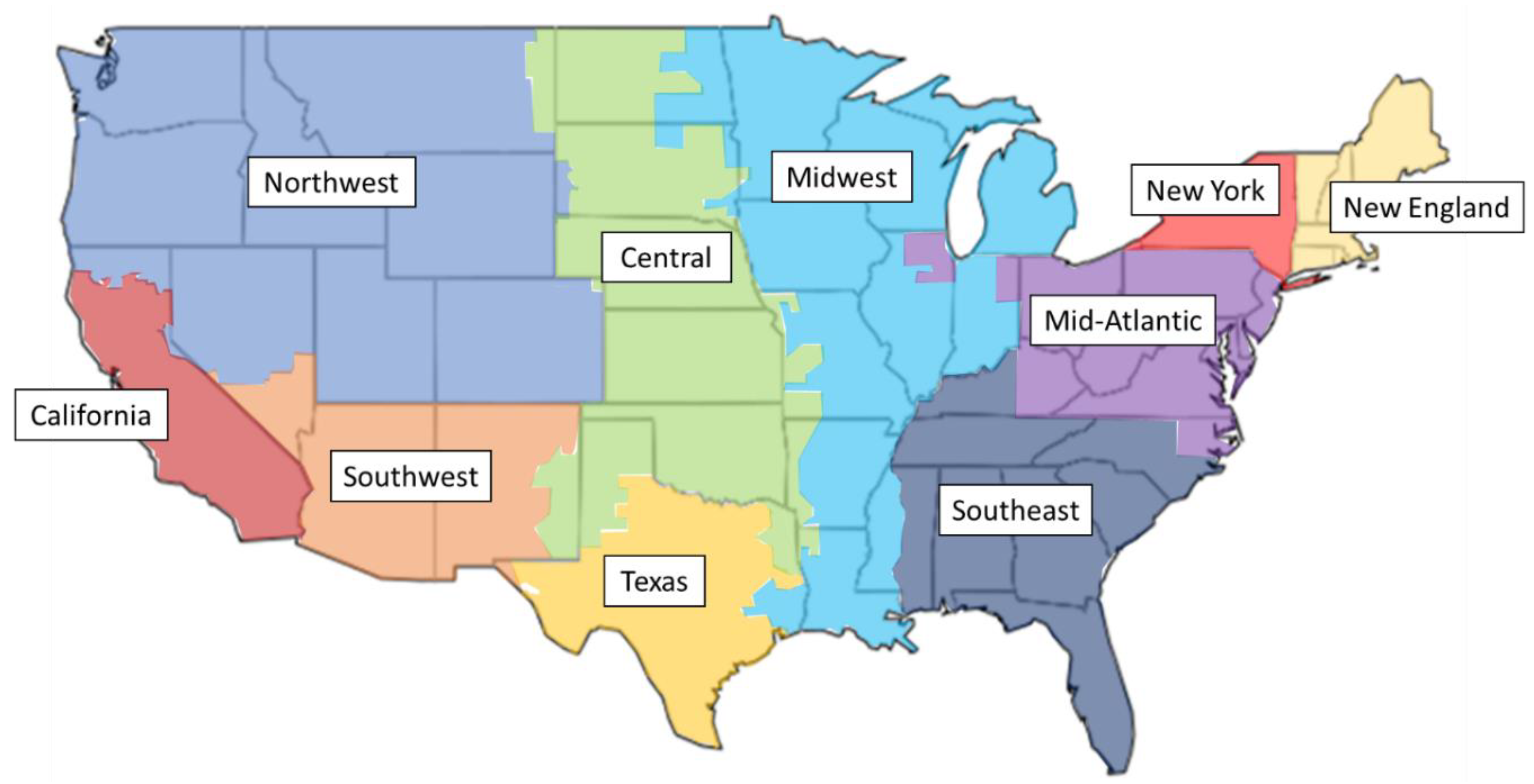
To study the short run effects of carbon policy, an electricity market optimization model was built. The model solves for hourly least-cost production levels across the U.S. given available power plants, transmission capacity, and operational constraints. The U.S. was separated into 10 regions that approximate existing electricity market boundaries, shown in Figure 1. Power plants are dispatched to meet hourly demand for each market region. Imports and exports between regions are constrained to approximate existing transmission capabilities between markets. Power plants are dispatched to satisfy exogenously provided and inelastic hourly demand. Inelastic demand is a reasonable assumption consistent with empirical evidence [36] because in the short run, most electricity consumers do not see changes in their electricity price. Incentive-based demand response resources are sometimes administratively deployed in real-time electricity auction markets [37]. However, these events rarely occur and as a result have minimal impact on the overall elasticity of electricity demand.
No transmission congestion within market regions is assumed. This is partly because the U.S. lacks a quality source of public data on sub-regional electric transmission lines. Abstracting from local transmission congestion also improves the model’s computational tractability. This means that any generator within a market region can serve demand anywhere in the same region. Areas that experience significant within-region transmission congestion would experience greater friction in the ability of their generators to respond to the policy, leading to higher costs and lower emissions reductions. The results provide useful broad insights, but due to the possibility of local constraints, meaningful conclusions about specific locales should incorporate a better understanding of local transmission congestion in that area. Integer constraints are avoided to ease the computational burden. This involves abstracting from non-linear components of power plant operations decisions, including start-up and shut-down costs, and minimum run times. This assumption means that offers are not temporally linked across hours, in the way a plant operator would consider the probable levels of future prices when deciding to start up a generator. Furthermore, the lack of start-up costs and ramping constraints in the model results in inflexible marginal generators ramping more frequently than what they would in reality. This is not an issue with nuclear plants as they are mostly inframarginal, however the model does cycle some marginally competitive coal units. The effects of this on the results are discussed in more detail in Section 3.5. Both local transmission congestion and non-linear operational constraints can have significant implications on any given power plant’s production schedules. For this reason, plant-level results are not emphasized.
Despite these simplifying assumptions, aggregated results from the model provide useful insights to policymakers at the national, regional, and state levels. The baseline scenario replicates aggregate levels of recently observed emissions, transmission levels, market prices, and generation reasonably well. Details from a baseline model validation exercise are discussed in Section 3.5. At the state level, Mann et al. [38] analyzed results from an electricity market model that similarly abstracts from transmission and non-linear power plant constraints for the state of Texas. They compared their results with highly detailed models that incorporate local transmission and power plant operational constraints, and found relatively consistent aggregate results between the simple and detailed models.
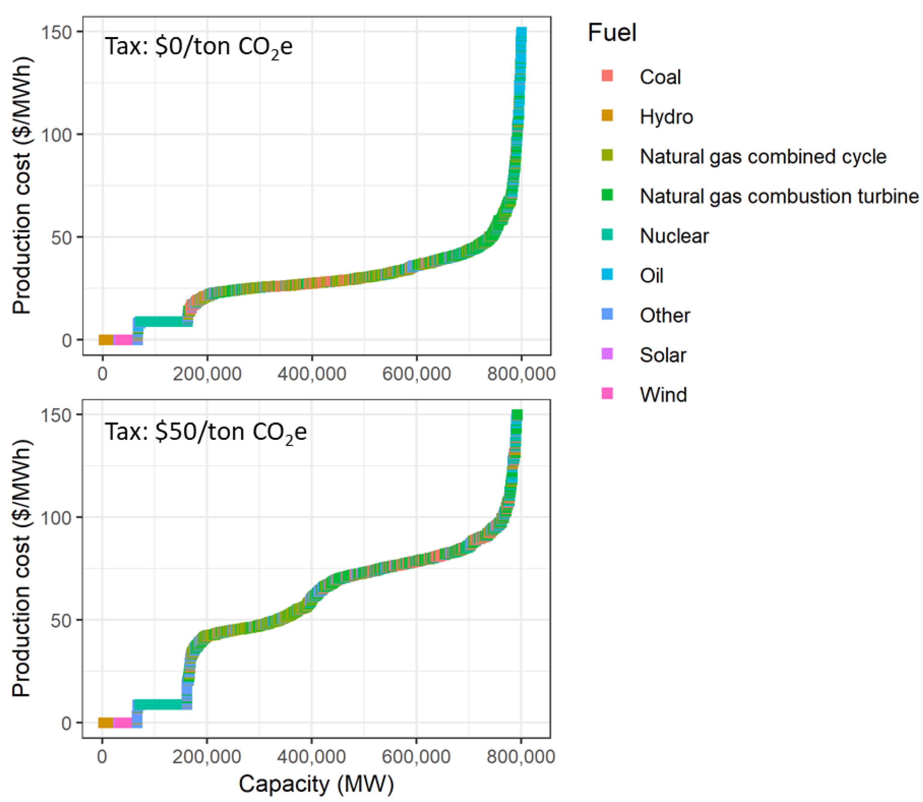
The carbon price is simulated as an increase in marginal costs proportional to each power plant’s observed CO2-equivalent (CO2e) emissions rate. After implementing the carbon price, the optimization re-orders supply curves in order of marginal costs. This is illustrated in Figure 2, which presents supply curves for all U.S. electricity generation with and without a carbon price. A carbon price shifts emitting electric generators up. The non-emitting forms of generation, including wind, solar, and hydro, do not shift vertically. The carbon price also shifts many natural gas power plants to the left, represented as the green portions of the curve, while shifting coal plants to the right, represented in red. This is because coal plants become relatively more expensive compared to natural gas after the policy. Coal plants have higher emissions intensities than natural gas and have to pay a higher carbon tax for every unit of electricity produced. Natural gas combined cycle plants emit 60% less greenhouse gases per unit than coal plants. Specifically, capacity-weighted average CO2e emissions rates for U.S. power plants are approximately 2194 lbs/MWh for coal plants and 899 lbs/MWh for natural gas combined cycle plants [39]. Thus, the primary mechanism through which a carbon price causes emissions reductions in the short run is from replacing coal generation with natural gas.
The electricity market model assumes competitive, cost-minimizing suppliers and inelastic demand. Theoretical evidence suggests these two market characteristics lead to 100% pass through of emissions costs to consumers. Sijm et al. [40] describes in detail the economic theory on emissions cost pass through in electricity markets. Consumers will purchase the same quantity of electricity in the short run no matter the price, because they are shielded from price changes. Competitive supply results in suppliers offering to sell electricity at their marginal production costs. When a tax is added to suppliers’ marginal costs, the full additional cost is reflected in their new offers, and consumers accept the price increase without reducing their quantity demanded. Consistent with this theory, Sijm et al. [41] found high levels of carbon price pass through into electricity prices in Europe. Woo et al. [42] also find relatively high (but less than 100%) carbon cost pass through into California electricity prices. They note their results are influenced by market distortions related to trading and emissions leakage into neighboring markets not covered by California’s carbon policy. If electricity market structures in the U.S. deviate from this model, it will tend to reduce the level of pass through to the electricity price. For instance, a market characterized by oligopoly supply and inelastic demand will have lower pass through because profit-maximizing firms’ marginal revenue functions are steeper than the demand curve.
3.2. Algebraic Model Formulation
This section presents an algebraic formulation of the electricity market model. The model utilizes the following parameters:
- maximum operating capacity of plant during month in megawatts ()
- production cost of plant in hour , in dollars per megawatt-hour ()
- carbon dioxide-equivalent emissions rate for plant , in
- demand in market region during hour , in
- hourly operating reserves in region in
- transmission capacity limit from region to region , measured in
- average net international imports into market region for month
- carbon price imposed by policy, in
The set of choice variables are the levels of hourly production from each plant, , and the levels of power transferred between each market region, , in . Each market region coordinates to minimize the cost of dispatching power plants across the United States, subject to capacity constraints and demand levels. In this way, the optimization problem is algebraically formulated as follows:
Subject to the following constraints:
The objective function in Equation (1) chooses hourly plant production and regional transmission flows to minimize production costs, including the carbon price. Equation (2) requires that production plus net imports from all other regions meet demand plus operating reserves in region , for all hours. Equation (3) limits production from each plant to be less than or equal to its total capacity, and non-negative. Equation (4) limits energy transfers across market regions to the available transmission capacity. Prices in the model are equal to the production cost of the marginal power plant for each hour in each market region. This is equivalent to the increase in system production cost if demand increased by a small amount. In mathematical optimization terms, this is the Lagrange multiplier of the demand constraints.
3.3. Data
The data used to construct the model are all publicly available and mostly downloaded from U.S. government websites. Power plant capacity limits () were obtained from the U.S. Energy Information Administration’s (US EIA) survey form 860 [43]. Each plant is assigned to one of 11 electric generation technology categories.. To incorporate the probability of power plants going offline for maintenance or unanticipated outages, capacity limits were discounted by corresponding average outage rates reported by the North American Electric Reliability Corporation (NERC) [44].
Capacity limits for wind and solar were determined from recently-observed average monthly output levels, calculated using US EIA historic generation data from form 923 [45]. These capacity limits adjust by month to capture seasonal variation in wind and solar outputs. Solar plants are allowed to generate during the day, and turn off at night. Hydro plant operators face complicated dispatch decisions that vary by year and season according to reservoir storage levels. Rather than attempt to incorporate this behavior in the model, hydro capacity limits are also set to recently-observed average output levels. While electricity markets experience variation in renewable energy output on any given day, Wan [46] presents empiric data from across the U.S. showing aggregated average wind outputs are fairly stable over 24-hour daily cycles. Furthermore, wind, solar and hydro plants rarely operate on the margin today and their daily dispatch levels would be relatively unaffected by a carbon policy. For these reasons, abstracting from hourly wind and solar variability and hydro dispatch decisions do not materially impact the aggregated estimates presented in Section 4 and Section 5.
Electricity production costs include the cost of fuel, operations, maintenance, and emissions. US EIA survey form 923 also reports monthly, generator-level fuel costs for fossil-fueled plants. Aggregated statistics of fuel costs for the remaining technologies and operations and maintenance (O&M) costs for all technologies were gathered from the U.S. National Renewable Energy Laboratory (NREL)’s Annual Technology Baseline dataset [47]. Plants that are located in California or the Regional Greenhouse Gas Initiative (RGGI) in the northeastern U.S. have greenhouse gas emissions costs in the baseline scenario. These existing carbon costs were obtained from The World Bank [48]. Recently observed electricity demand levels () and regional transmission flows from the US EIA’s electric system operating data were used [49]. Public data on transmission capacity () is not available. Instead, capacity levels were set to recently observed average transmission flows. International trade of electricity into and out of markets is provided exogenously, and determined by monthly-averaged flows across the Canadian and Mexican borders. Some market regions rely on significant levels of imports. New England and New York have the highest levels of import intensity, with annually-averaged international net import levels of approximately 10% and 6% of annual peak demand, respectively.
Operating reserves () are included to reflect uncertainty in electricity demand and generation output. They are set to equal 3% of demand plus 5% of average wind and solar output for each region and hour. This “3+5” heuristic was determined by GE and NREL [50] to perform well for temporally-granular electricity market models. Power plant emissions rates () were calculated using recently observed plant-level emissions data from the U.S. Environmental Protection Agency (US EPA) [39]. US EPA reports CO2-equivalent (CO2e) emissions rates. These rates standardize and incorporate the global warming potentials of methane (CH4), nitrous oxide (N2O), and sulfur hexafluoride (SF6) released by power plants, in addition to CO2. However, approximately 98% of total U.S. electricity CO2e emissions are CO2. The methodology for calculating CO2e levels is described on page 18 of US EPA (2016)’s eGRID technical documentation [51].
3.4. Model Construction and Solution Procedure
The model was solved as a set of linear programs using the open-sourced LPSolve software. LPSolve is a revised simplex and branch-and-bound mixed-integer linear program solver [52]. The solver is accessed using a wrapper function in R [53]. R is a free, open-sourced, object-oriented programming language and computing environment [54]. To understand how the model is coded and solved it is useful to think like the computer in terms of operations on data in matrices and vectors. Therefore, this section supplements the algebraic model formulation in Section 3.2 with a more detailed model description using matrix and vector notation. The model is solved as a single linear program for each hour, so the data objects described herein are indexed by hour (for example, ). As described in Section 3.2, some model inputs vary hourly (production costs and demand ), some vary monthly (plant capacity constraints ), and others do not vary at all (transmission capacity limits and the relations described by the constraint coefficients included in matrix ). All the information necessary to fully describe how model variables change over time were provided in Section 3.2. The time subscripts for data objects are omitted from the following description to reduce clutter.
The linear program is solved in the following standard format:
where is the vector of choice variables, is the vector of objective function coefficients, is the matrix of constraint coefficients, and is the vector of scalars on the right side of the constraint equations. In this application, includes the vector of power plant production decisions plus transmission levels . There are power plants in the dataset. There are also possible transmission connections between market regions, because each of the 10 regions has nine potential trading partners. In the U.S., several pairs of market regions do not have any physical transmission connections between them, in which case the associated transmission capacity is constrained to be zero. In total, has non-negative elements (), and is arranged as follows:
The vector includes plant-level variable production costs, followed by transmission costs, in . Production costs for each plant include fuel costs, variable operations and maintenance costs, and baseline carbon costs for plants in the California and RGGI regions. Carbon prices are added to for the carbon policy scenarios. Transmission costs are assumed to be equal across all market regions. Future applications could explore the implications of heterogeneous transmission costs between market regions, if public transmission cost data became available.
The vector includes the right-hand-side values of all the constraints. The first elements represent the capacity constraints for each plant , followed by the transmission constraints . This is followed by demand constraints , which are equal to demand plus operating reserves minus international imports for each market region. Thus, has elements (), and is arranged as follows:
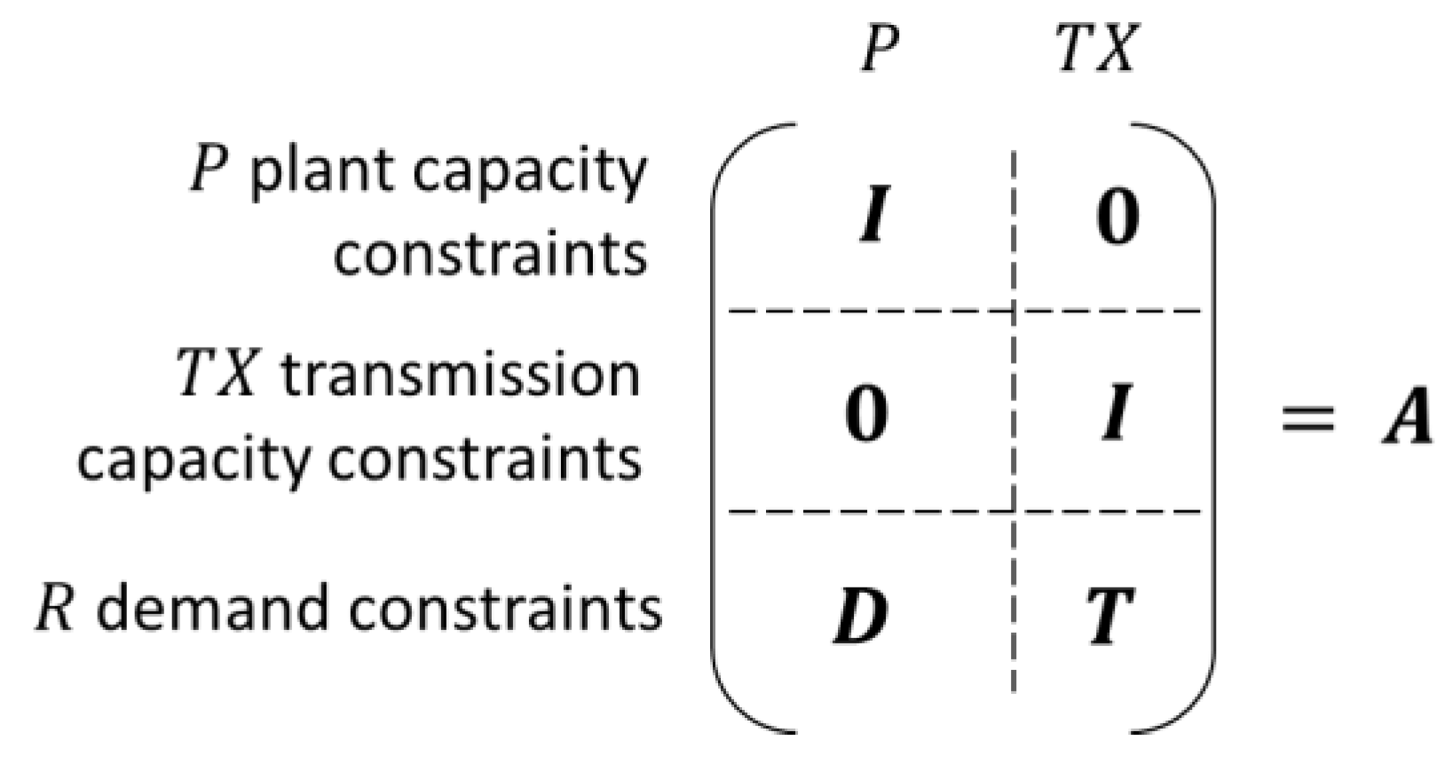
The matrix includes the constraint coefficients, with each of the rows corresponding to a constraint equation. In explaining the construction of the constraint coefficient matrix, it is useful to separate it into the block matrix shown in Figure 3. The dimensions for each of the six submatrices are described on the outside. The first rows in correspond to the plant capacity constraints in the vector . They are constructed by column-binding an identity matrix () of order with a zero matrix (0) of dimensions . The following rows correspond to the 90 transmission constraints that follow in . This is constructed by column-binding a zero matrix with an identify matrix of order .
The final rows in Figure 3 correspond to the demand constraints, one for each market region. Within these final rows, the submatrix is built by assigning to each element whose column corresponds to a plant in the region corresponding to row (). Furthermore, the submatrix is built by assigning 1 to each element whose column represents a transmission flow into the region corresponding with row (). In this way, the elements are assigned according to Equation (8). This ensures that for each hour, the elements of are chosen such that the sum of all plants and transmission imports meets demand for each market region.
The last input required for the model is a constraint direction vector of length defining the direction of each inequality constraint. The choice variables and must be less than or equal to the plant and transmission capacity constraints, and the sum of supply plus imports must be greater than or equal to demand. In this way, the first elements of the constraint direction vector are “” while the last elements are equal to “”.
3.5. Baseline Scenario
A baseline scenario without a national carbon policy was solved, and the model was validated by comparing the outputs to recently observed data. Model-estimated annual CO2e emissions from electricity production in this baseline scenario were 1.62 billion metric tons. The US EPA-reported CO2e emissions from the power sector in 2017 were 1.78 billion [55]. This difference stems from the fact that the EPA’s greenhouse gas inventory includes all stationary combustion emissions related to the generation of electricity. US EIA’s form 860, the dataset providing the power plants used in the model, covers electric power plants with 1 megawatt (MW) or greater of combined nameplate capacity. Greenhouse gas emissions from small electric generators will show up in EPA’s inventory but not in EIA’s inventory, and as a result will not be included in the model.
Model-estimated electricity prices were compared with recently observed prices in market regions that report such data [56]. This comparison is reported in Table 1. Modeled prices closely match observed prices, except for divergences in California and New England. In these two regions, modeled prices are significantly higher than what has been recently observed. This is likely because California and New England have high levels of low-cost distributed electricity generation that are not picked up by the datasets underlying the model. For example, California and New Jersey have the highest levels of electricity production from small-scale solar plants less than 1 MW in nameplate capacity among all states [57]. Again, US EIA’s form 860 dataset covers electric power plants larger than 1 MW of combined nameplate capacity, so these distributed generators are not included in the model. Incorporating distributed generation would result in a rightward shift of the supply curves (or leftward shift in net demand curves) for these two regions, lowering equilibrium prices. Fortunately, the short run relative economics between natural gas and coal plants after a carbon price that underly the results of this study are not significantly impacted by distributed solar, and these divergences in California and New England will not significantly alter the results.
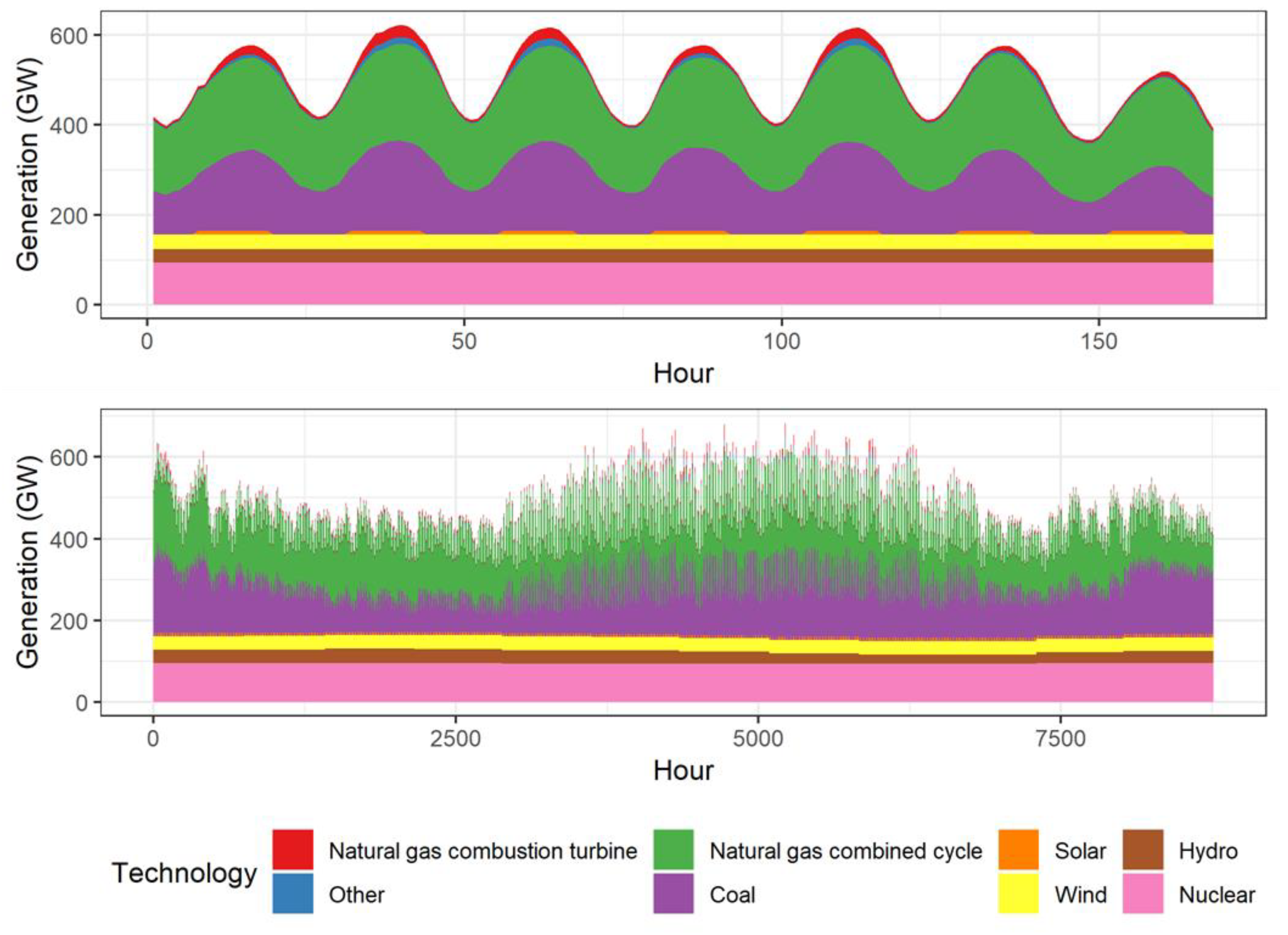
Next, modeled generation levels for dispatchable technologies were aggregated by fuel type and compared to aggregate observed generation levels reported in the EIA form 923 dataset. Modeled generation levels are compared to observed levels from recent years in Table 2. The comparison shows the model slightly under-predicts coal generation compared to the observed level. In the model, a significant fraction of coal units are ramped down on a daily basis during low-demand hours when they are not economically competitive. Cost-competitive combined cycle natural gas plants replace the coal generation that ramps down. Figure 4 plots modeled electricity production by fuel source for one week and a full year, and shows the daily cycling dynamics of these two fuel sources. This daily cycling may be causing the model to underpredict coal generation due to non-competitive market conditions and generator ramping costs not considered in the model. For example, in some markets it is relatively common for coal plants to self-schedule and produce even if their offer exceeds the system’s marginal cost. During these periods, wind and solar may be curtailed instead of coal if supply exceeds demand.
Table 2 also shows modeled production from natural gas combustion turbine plants is less than recently observed levels. Combustion turbines are primarily dispatched during periods with high market prices and tight supply conditions. This is likely due to the deterministic model under-predicts unplanned contingencies that cause high prices, including the unexpected loss of a large generator or transmission line.
As discussed in Section 3.3 and shown in Figure 4, wind, solar, and hydro are modeled by setting production equal to each plant’s recently observed output level. This approach results in accurate aggregate levels of wind and solar production, while abstracting from the complicated, weather-driven hourly variation characteristic of wind and solar production profiles and seasonal, reservoir-driven production of hydro. Profit-maximizing owners of these technologies will offer to sell in a competitive electricity market at close to zero dollars because they do not have fuel costs and have low marginal production costs. As a result, these power plants are rarely on the margin, and the operator’s decision to schedule cost-effective wind, solar, and hydroelectricity will not change in the short run due to a carbon price. Rather, the majority of short run effects from the carbon price come from relative changes in production costs between coal and natural gas combined cycle generation. Combined cycle natural gas generation replaces coal generation on the margin after a carbon price because it has a lower greenhouse gas emissions intensity.
The conclusions from this model validation exercise provide confidence in the study’s overall results. Electricity prices predicted by the model match recently observed electricity prices for most regions where data is available. The modeled prices deviate from observed levels in California and New England due to significant levels of distributed generation not captured by the model. There are also relatively small deviations between coal and natural gas generation predicted by the model, explained by non-competitive market conditions that are not modeled. The change in short run relative economics between coal and natural gas from a carbon policy is the most important factor driving the short run effects. If one can accept the reasonable assumption that effects from these operational and non-competitive dynamics remain constant for a short period of time after a carbon price is implemented, then the overall implications of these deviations on the quality of results are minor. This type of assumption is commonly invoked when attempting to understand and model economic phenomena. It is often referred to by the Latin phrase “ceteris paribus,” translated to “holding all else constant.”
4. Discussion
4.1. Overall Results
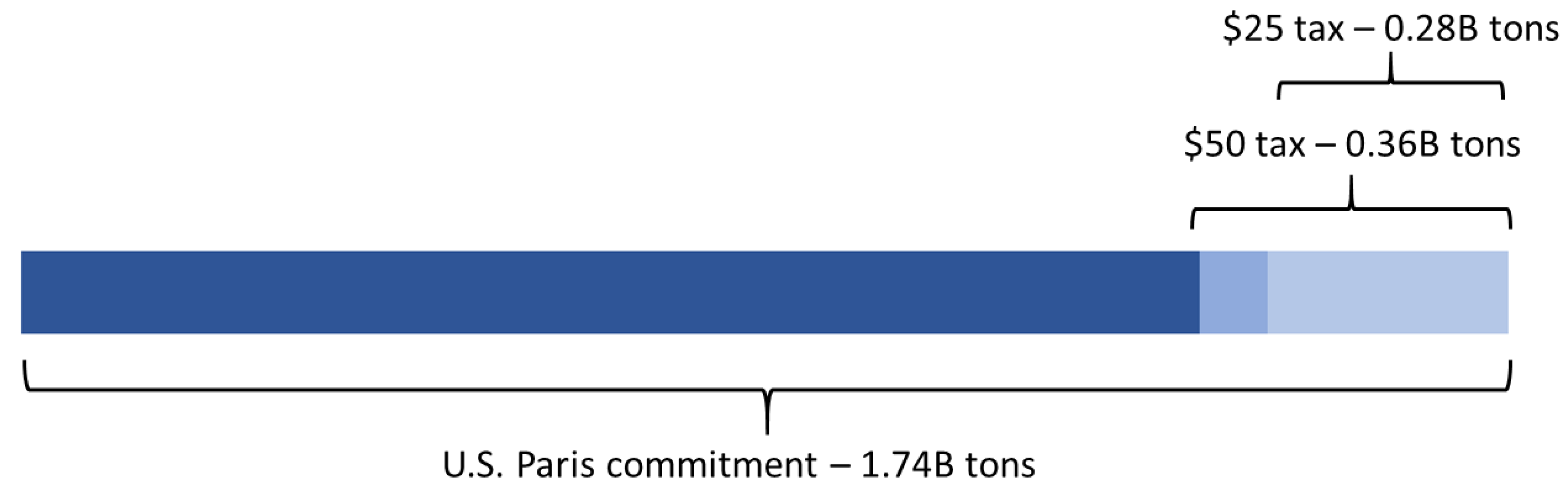
The model predicts short run decreases in annual electricity sector CO2e emissions from current levels of 17% from a $25/ton carbon tax and 22% from a $50/ton carbon price. The emissions levels for the three modeled scenarios are displayed in Table 3. There were 5.7 billion total tons of U.S. CO2e greenhouse gas emissions emitted in 2017 [55]. The simulated electricity emissions reductions are equivalent to 4.9% and 6.3% reductions in economy-wide greenhouse gas emissions for the $25 and $50 case, holding emissions from all other industries constant. The short run electricity emissions reductions from a $50/ton tax are equivalent to approximately 21% of the U.S.’s voluntary 2025 greenhouse gas reduction commitment under the Paris Climate Accord [58]. This calculation is presented visually in Figure 5. The short run electricity greenhouse gas emissions reductions estimates come from operational changes to the existing capital stock. They do not include additional long run emissions reductions caused by new investments in low-carbon electricity production and retirements of high-carbon electricity production assets caused by the policy.
These results suggest significant short run emissions reductions can be achieved from a U.S. carbon price on the electricity sector. The tax on these emissions generates $33.5 billion in government revenue in the $25 scenario, and $63.0 billion in the $50 scenario.
Almost all of the short run emissions reductions come from switching electricity fuel consumption from coal to natural gas. As discussed in Section 3.4, this is because most marginal electricity production in the U.S. is produced from one of these fuels, and a carbon price will have a relatively large immediate effect on the short run marginal costs of coal and natural gas power plants. Table 4 displays total generation from coal and natural gas generation in each of the three scenarios. It shows the model estimates a 43% short run reduction in U.S. coal generation from a $25/ton carbon price, and a 59% reduction from a $50/ton price. Much of this is offset by increased natural gas generation of 30% and 40% in the two scenarios, respectively.
The results also suggest a carbon price will have significant short run price effects in wholesale electricity markets. The largest price impacts occur in coal-heavy markets including the Central, Mid-Atlantic, and Midwest regions. Table 5 presents average prices by scenario broken out by market region. The column ‘$50/ton—Baseline’ displays the change in price after implementing a $50/ton price. The final column displays emissions elasticity of price, calculated as the percent change in total regional emissions divided by the percent change in average price. This calculation provides insight into the short run cost-effectiveness of emissions reductions. A lower number indicates a larger emissions decrease relative to its increase in price. The Northwest region has the lowest value, showing that a 1% increase in average price is associated with a 0.35% decrease in regional emissions due to the policy. The positive value for California represents the fact that both price and emissions increased as a result of the carbon policy.
The price impacts are qualified by the fact that these are first order effect estimates derived from short run supply side adjustments to the carbon price. In the electricity industry, most customers are insulated from short run price changes through long term contracts and regulator-approved retail electricity prices. These price increases will eventually be offset by downward pressure from reduced demand and new investments in electricity supply, both of which are second-order effects not considered in the model.
Transmission flows adjust so that regions which experience relatively larger increases in marginal production costs after the carbon price import more energy from less-affected regions. Table 6 presents average transmission flows across regions in the baseline and $50/ton scenarios. The most striking impact is in the Northwest region. Electricity trade from the Northwest to California dropped to approximately one-third of the baseline level, offset by a trade reversal from California and the Southwest region. Ample transmission capacity between these three regions, along with relatively more cost-competitive natural gas capacity across the Western U.S. after the carbon price, resulted in the Northwest drastically reducing coal generation in the $50 scenario to one-fifth of its baseline level. These results are qualified by the fact that there are hydroelectric production constraints across the west that are not modeled but determine in part regional trade. Furthermore, there are market structures and contractual relationships across the west and other regions that are not modeled but tend to reinforce status quo levels of regional trade in the short run [59].
4.2. State-Level Results
Implementing a national carbon price in the U.S. would most likely occur after political negotiation and compromise among state representatives in the U.S. Congress. Understanding state-level impacts is politically important for developing national carbon policy. This section analyzes state impacts on emissions, generation, costs, and tax revenue. Table 7 at the end of this section displays a comprehensive set of model results for each state. The results in Table 7 are discussed more fully with multiple references throughout this section.
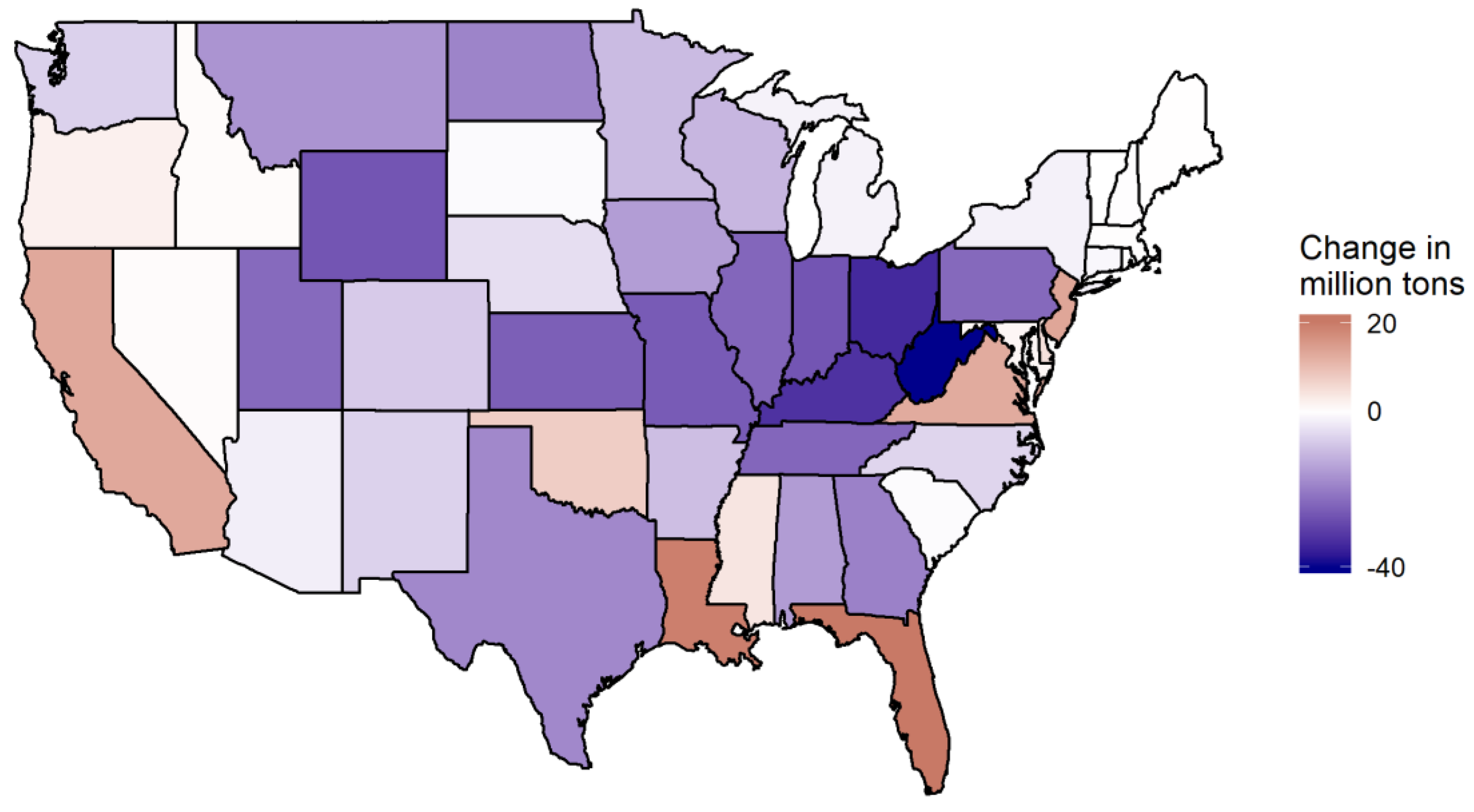
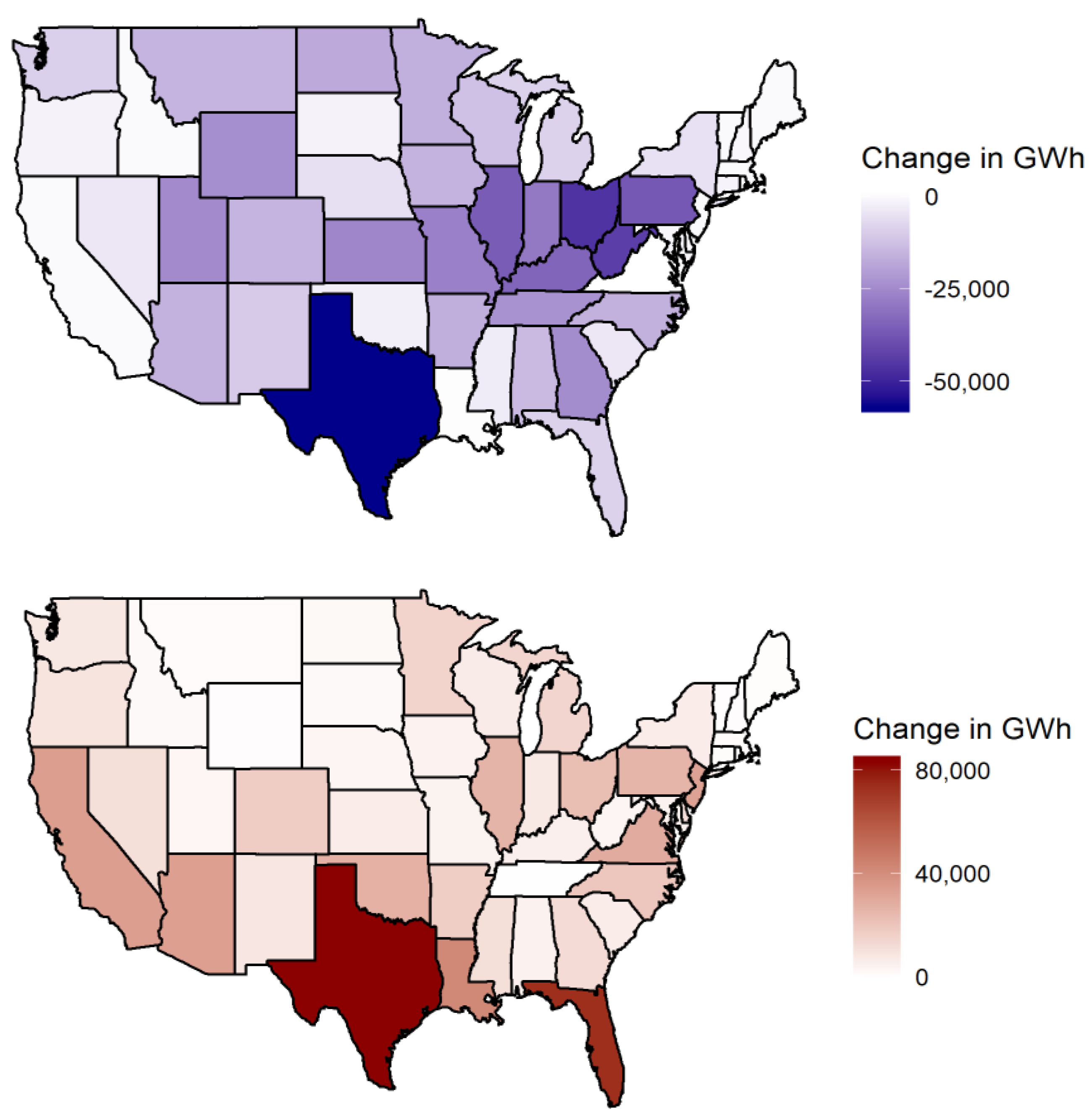
Figure 6 maps changes in CO2e emissions by state after simulating a $50/ton price. These correspond to the ‘CO2e’ columns in Table 7. Most net emissions reductions at the state level occur in coal-heavy states that are part of large regional markets, including West Virginia, Ohio, and Kentucky. These states reduce coal production and replace it with lower-carbon electricity production from neighboring states. Perhaps surprisingly, the cost-minimizing response to a federal carbon price involves increasing emissions in several states, including California, Florida, and Louisiana. These net emissions increases occur in states that are increasing natural gas production to offset coal reductions in neighboring states. This can be seen more explicitly in Figure 7., which maps state-level changes in coal and natural gas generation (the ‘Coal’ and ‘Gas’ columns in Table 7.). For example, West Virginia has a relatively large coal decrease and small natural gas increase. On the other hand, California increases natural gas generation but does not increase coal because the state has almost zero coal generation before the carbon policy. Political goals of individual states may interfere with the cost-minimizing short run policy response estimated by the model. Many states have individual greenhouse gas emissions reductions programs. For example, California’s greenhouse gas policies could prevent an increase in emissions after a carbon price, which would likely lessen the emissions reductions achieved in neighboring states. States which are predicted to have large emissions reductions, like West Virginia and Ohio, have large coal industries, which may be politically organized such that they can mitigate their industry’s decline and achieve lower emissions reductions. A detailed analysis of the political economy for each state would be important to further understanding the prospects of carbon policy.
Examining changes in electricity production costs by state provides additional insights into the effects of carbon policy. Production costs include the fuel, operations, maintenance, and emissions costs needed to produce electricity. They are equal to the area under the electricity supply curve, including the curves previously displayed in Figure 2. State production costs decrease when coal generation decreases, and increase when natural gas generation increases. These production costs should not be interpreted as net costs to society from the carbon policy. Rather, they provide insights into the magnitude of shifts in generation between fuel types and across states. As described in more detail in Section 3, the model assumes suppliers minimize costs and sell in a competitive market. As a result, suppliers would not incur production costs if there was not adequate revenue available in the market to cover their costs.
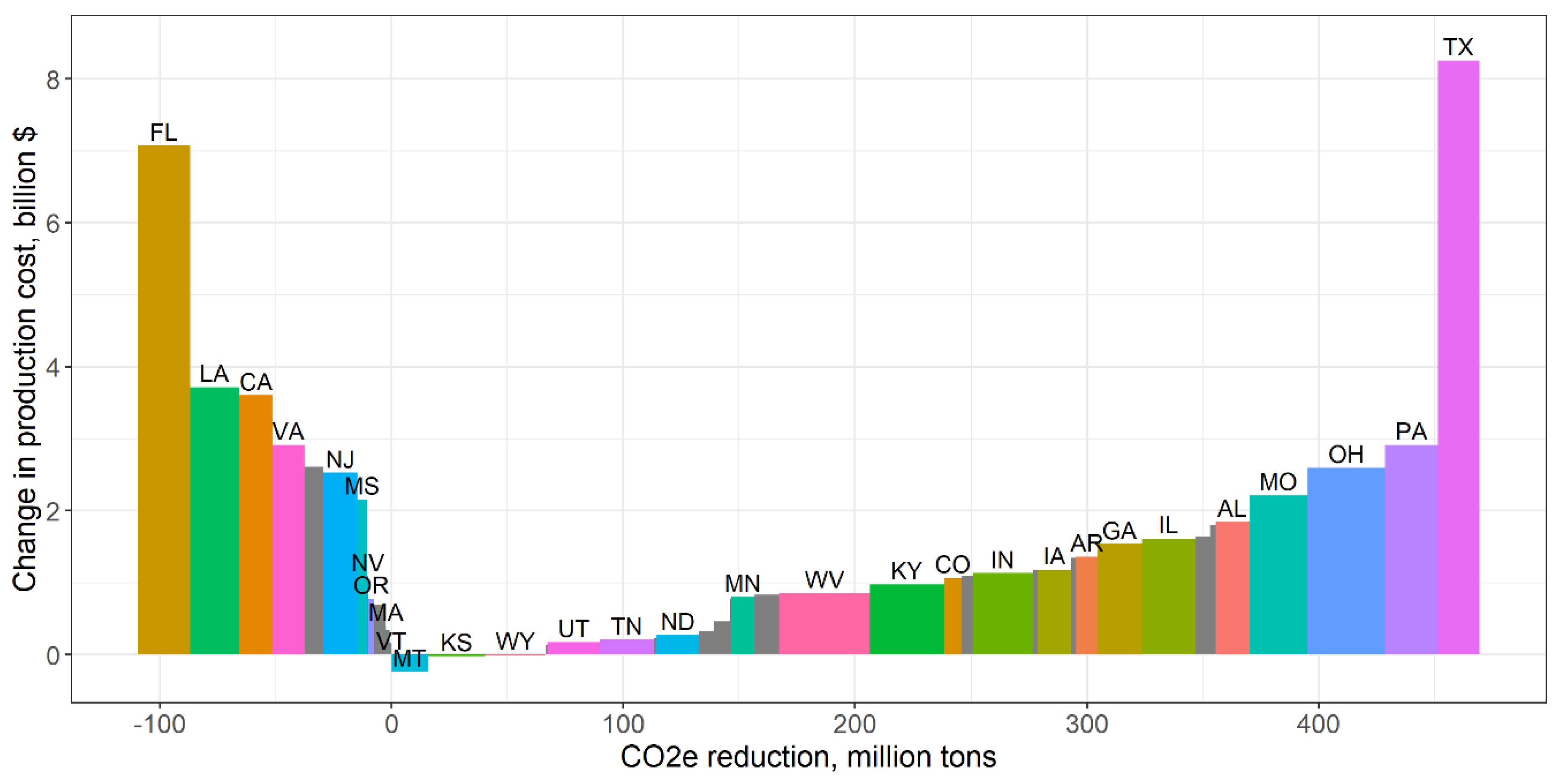
Figure 8 plots the change in production costs by state on the vertical axis as a result of a $50/ton price. The horizontal axis displays the state’s reduction in CO2e emissions from a $50/ton price. The width of each bar is proportional to the magnitude of emissions reduction. States that increase emissions are located to the left of zero on the horizontal axis, while states to the right of zero reduced emissions. State-level production cost changes correspond to the “Cost” columns in Table 7. Figure 8 shows a few interesting results. All states to the left of the origin increased emissions after a carbon tax, because they increased natural gas generation after a carbon price to serve demand in neighboring states. Montana experienced a net decrease in electricity production costs after a $50/ton carbon tax, even though all emitting electricity production became more expensive. This occurred because Montana coal producers decreased production while out-of-state electricity producers increased generation to make up the deficit. Both Florida and Texas had large increases in natural gas generation combined with large in-state electricity consumption, leading to their relatively large production costs increases.
All states that have emitting electricity production generate federal government revenue from the carbon tax. Tax revenue collected by state is displayed in the ‘Tax’ columns in Table 7. The highest revenue-generating states in the $50/ton scenario are Texas, Florida, and California at $7.0, $4.6, and $3.3 billion per year, respectively. The revenue raised by a carbon tax could be rebated as an equal lump sum to all U.S. citizens. This policy proposal is motivated by income inequality concerns and the desire to make a carbon tax revenue neutral. The $63 billion raised from the electricity industry in the $50/ton scenario would result in approximately $194 per person per year in rebates.
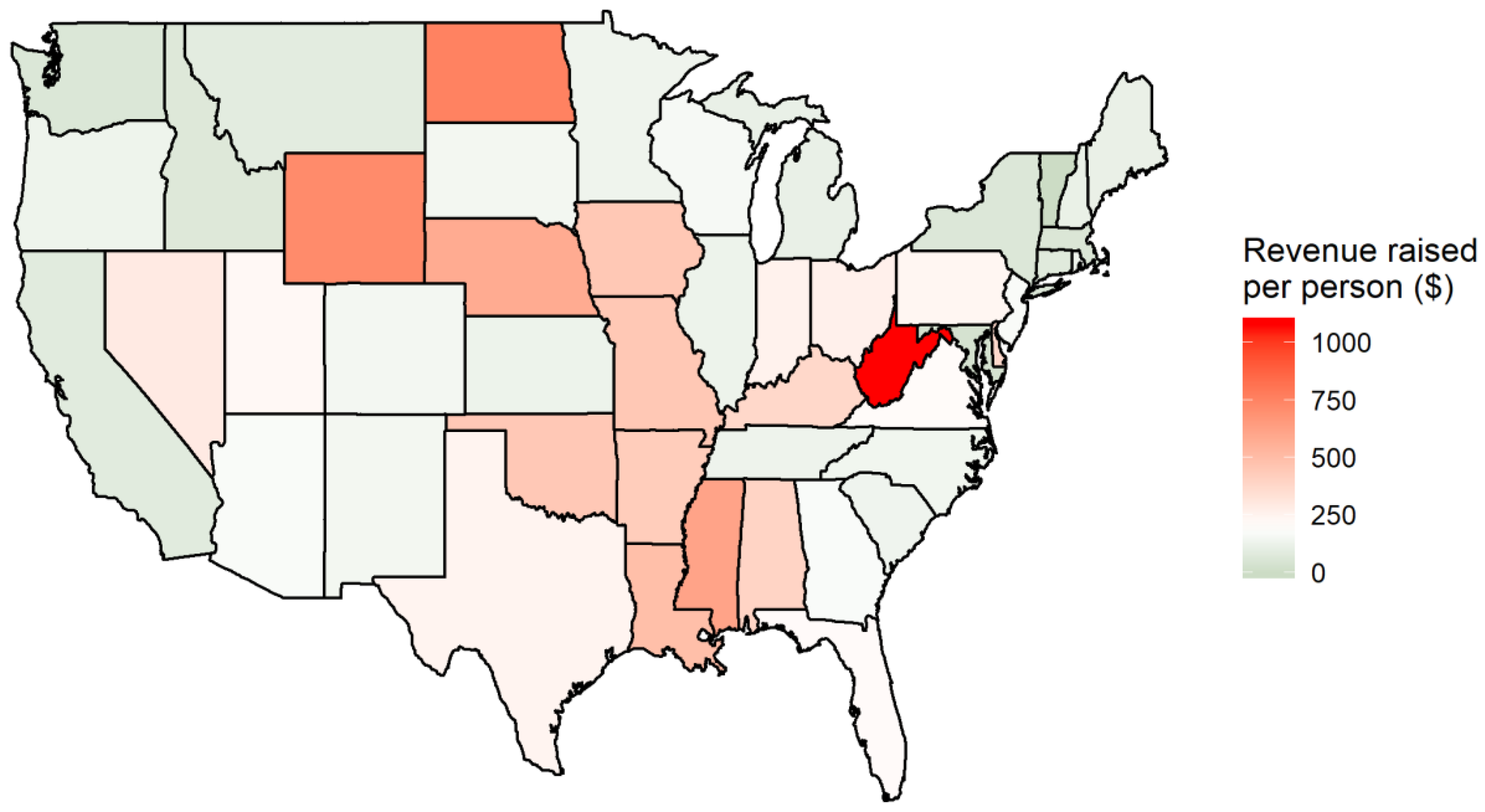
A flat rebate is contrasted with the fact that per capita tax revenue varies across states. This results in wealth transfers between states. States with high populations and/or low-emitting electricity are likely to pay less in carbon taxes than the per capita rebate their citizens receive. In the $50/ton scenario, all U.S. citizens receive a $194 rebate per year. However, residents of California and New York pay only $82 and $62 carbon tax per person, respectively, while residents of West Virginia pay $1077 per person. State population data for 2018 from the U.S. Census Bureau were used in these calculations [60]. Figure 9 displays taxes per person for the $50/ton scenario by state, and is color-coded to highlight the wealth transfer across states. On the color scale, the flat rebate of $194 is set to white. States that pay less than $194 in per capita carbon tax are on the green portion of the spectrum, while states that pay more than $194 per capita are on the red portion. In general, Figure 9 shows that a flat per capita rebate of electricity carbon tax revenue redistributes wealth from states in the middle of the country to states near the east or west coasts, with several exceptions.
One could assume that members of Congress will vote for a carbon tax and rebate policy if their state’s constituents receive a short term net benefit from the rebate. These are the states tinted green in Figure 9. In this case the policy would receive 54 votes in the Senate (a 56% majority) and 254 votes in the House of Representatives (a 59% majority), not including the legislators from Hawaii and Alaska, and be implemented into law.
The tax revenue results suggest a negative relationship between a state’s wealth and their per capita carbon tax revenue. The correlation coefficient between a state’s 2018 gross state product and the per capita revenue in the $50/ton scenario is −0.27. While correlation does not imply causation, it can be speculated from this empirical observation that states with wealthier citizens are more likely to demand cleaner energy production, or import dirty energy from neighbors, to avoid experiencing the harmful effects of air pollution. As a result, the wealthier states would have a lower carbon tax burden, and receive a relatively higher benefit from a per capita revenue rebate.
5. Conclusions
This paper presents results from an electricity market model built to estimate short run effects of a U.S. carbon price. The results suggest a modest carbon tax can cause significant short run greenhouse gas emissions reductions from the U.S. electricity sector. The model estimates a $25/ton tax leads to 17% emissions reductions and a $50/ton tax leads to 22% reductions from current levels of electricity emissions. These are equivalent to approximately 4.9% and 6.3% reductions from current economy-wide greenhouse gas emissions. The estimated emissions reductions from a $50/ton electricity industry carbon tax represent 21% of the U.S.’s 2025 voluntary commitment under the Paris Climate Accord, holding emissions from all other industries constant.
The electricity market model captures short run operational changes to existing power plants caused by the carbon price. The majority of emissions reductions come from decreased coal consumption replaced with increased natural gas consumption. The model keeps the electricity capital stock fixed. The results do not include additional long run emissions reductions due to increased investments in low carbon-emitting production and increased retirements of high-carbon emitting power plants. The model assumes inelastic, exogenous demand and does not capture long run emissions reductions from decreased demand. Demand response is considered a long run dynamic because the short run elasticity of electricity demand is low, and most electric utilities in the U.S. pass changes in costs through to retail prices faced by customers over periods of several years.
I consider a scenario in which carbon tax revenues are rebated on a flat per capita basis to all U.S. citizens, consistent with recently proposed legislation in the U.S. Congress. Short run electricity carbon tax revenues in a $50/ton scenario raise approximately $194 per citizen. An electricity carbon tax is characterized by heterogeneous per capita tax revenue across states. As a result, a flat per capita rebate will cause a transfer of wealth from electricity consumers in high revenue per capita states to low revenue per capita states. These results are mapped in Figure 9, and in general involve transfers from relatively high-emitting, low-population states in the middle of the country to low-emitting, high-population states on the east and west coasts.
Most emissions reductions come from states that consume large amounts of coal in the Mid-Atlantic, Midwest, and Western U.S. The highest emissions reducing states include West Virginia, Ohio, Kentucky, Wyoming, and Indiana. The cost-minimizing response to a carbon tax involves increased emissions from several states. These states increase natural gas consumption to export electricity to and replace coal consumption in neighboring states that becomes more expensive after the carbon price. States that increase emissions in response to the carbon policy do so to enable a larger amount of lower-cost emissions reductions from their neighbors. If were not allowed, states that consume large amounts of coal would achieve less emissions reductions, and the country would experience higher costs from a carbon policy.
Funding
This research received no external funding.
Acknowledgments
The author would like to thank the following people for their support in the development of this work: My Ph.D. advisory committee members from Colorado School of Mines for their review of an early stage work scope: Ben Gilbert, Ian Lange, Peter Maniloff, and Paulo Cesar Tabares-Velasco; Dustin Mulvaney and other participants in the San Jose State University Environmental Studies research seminar for their research feedback; participants in the May, 2019 meeting of the San Francisco Bay Area R User Group, for their thoughtful questions and feedback on the modeling methods; Jack Moore, Zachary Ming, and Stefanie Tanenhaus from Energy + Environmental Economics, Inc, for their feedback on an early-stage work scope.
Conflicts of Interest
I declare no conflict of interest.
References
- Nordhaus, W.D. Optimal Greenhouse-Gas Reductions and Tax Policy in the ‘DICE’ Model. Am. Econ. Rev. 1993, 83, 313–317. [Google Scholar]
- Fankhauser, S. The Social Costs of Greenhouse Gas Emissions: An Expected Value Approach. Energy J. 1994, 15, 157–184. [Google Scholar] [CrossRef]
- Tol, R.S.J. Estimates of the Damage Costs of Climate Change. Part 1: Benchmark Estimates. Environ. Resour. Econ. 2002, 21, 47–73. [Google Scholar] [CrossRef]
- Hope, C. The marginal impact of CO2 from PAGE2002: An integrated assessment model incorporating the IPCC’s five reasons for concern. Integr. Assess. 2006, 6, 19–56. [Google Scholar]
- Stern, N.; Stern, N.H.; Treasury, G.B. The Economics of Climate Change: The Stern Review; Cambridge University Press: Cambridge, UK, 2007. [Google Scholar]
- Tol, R.S.J. Targets for global climate policy: An overview. J. Econ. Dyn. Control 2013, 37, 911–928. [Google Scholar] [CrossRef] [Green Version]
- Zhang, K.; Wang, Q.; Liang, Q.-M.; Chen, H. A bibliometric analysis of research on carbon tax from 1989 to 2014. Renew. Sustain. Energy Rev. 2016, 58, 297–310. [Google Scholar] [CrossRef]
- Weitzman, M.L. Prices vs. Quantities. Rev. Econ. Stud. 1974, 41, 477–491. [Google Scholar] [CrossRef]
- Newbery, D. Policies for decarbonizing a liberalized power sector. Econ. Open-Access Open-Assess. E-J. 2018, 12, 2018-40. [Google Scholar] [CrossRef]
- Ackerman, F.; Stanton, E.A. Climate Risks and Carbon Prices: Revising the Social Cost of Carbon. Econ. Open-Access Open-Assess. E-J. 2012, 6, 2012-10. [Google Scholar] [CrossRef]
- Greenstone, M.; Kopits, E.; Wolverton, A. Developing a Social Cost of Carbon for US Regulatory Analysis: A Methodology and Interpretation. Rev. Environ. Econ. Policy 2013, 7, 23–46. [Google Scholar] [CrossRef] [Green Version]
- Kaufman, N. How the Bipartisan Energy Innovation and Carbon Dividend Act Compares to Other Carbon Tax Proposals; A Commentary; Columbia SIPA Center on Global Energy Policy: New York, NY, USA, 2018. [Google Scholar]
- Jorgenson, D.W.; Wilcoxen, P.J. Reducing US carbon emissions: An econometric general equilibrium assessment. Resour. Energy Econ. 1993, 15, 7–25. [Google Scholar] [CrossRef]
- Goulder, L.H. Effects of Carbon Taxes in an Economy with Prior Tax Distortions: An Intertemporal General Equilibrium Analysis. J. Environ. Econ. Manag. 1995, 29, 271–297. [Google Scholar] [CrossRef]
- Rausch, S.; Metcalf, G.E.; Reilly, J.M. Distributional impacts of carbon pricing: A general equilibrium approach with micro-data for households. Energy Econ. 2011, 33, S20–S33. [Google Scholar] [CrossRef] [Green Version]
- Macaluso, N.; Tuladhar, S.; Woollacott, J.; Mcfarland, J.R.; Creason, J.; Cole, J. The impact of carbon taxation and revenue recycling on U.S. industries. Clim. Chang. Econ. 2018, 9, 1840005. [Google Scholar] [CrossRef]
- Chen, Y.; Hafstead, M. Using a carbon tax to meet U.S. international climate pledges. Clim. Chang. Econ. 2019, 10, 1950002. [Google Scholar] [CrossRef]
- Barron, A.R.; Fawcett, A.A.; Hafstead, M.; Mcfarland, J.R.; Morris, A.C. Policy insights from the EMF 32 study on U.S. carbon tax scenarios. Clim. Chang. Econ. 2019, 9, 1840003. [Google Scholar] [CrossRef]
- Nicholson, M.; Biegler, T.; Brook, B.W. How carbon pricing changes the relative competitiveness of low-carbon baseload generating technologies. Energy 2011, 36, 305–313. [Google Scholar] [CrossRef]
- United States Environmental Protection Agency (US EPA). Sources of Greenhouse Gas Emissions. In US EPA; 29 December 2015. Available online: https://www.epa.gov/ghgemissions/sources-greenhouse-gas-emissions (accessed on 29 March 2019).
- Schäfer, A.; Jacoby, H.D. Technology detail in a multisector CGE model: Transport under climate policy. Energy Econ. 2005, 27, 1–24. [Google Scholar] [CrossRef]
- Mendelsohn, R.; Nordhaus, W.D.; Shaw, D. The Impact of Global Warming on Agriculture: A Ricardian Analysis. Am. Econ. Rev. 1994, 84, 753–771. [Google Scholar]
- Darwin, R. Effects of Greenhouse Gas Emissions on World Agriculture, Food Consumption, and Economic Welfare. Clim. Chang. 2004, 66, 191–238. [Google Scholar] [CrossRef]
- Martin, R.; de Preux, L.B.; Wagner, U.J. The impact of a carbon tax on manufacturing: Evidence from microdata. J. Public Econ. 2014, 117, 1–14. [Google Scholar] [CrossRef] [Green Version]
- Berrittella, M.; Bigano, A.; Roson, R.; Tol, R.S.J. A general equilibrium analysis of climate change impacts on tourism. Tour. Manag. 2006, 27, 913–924. [Google Scholar] [CrossRef] [Green Version]
- Murray, B.C.; Bistline, J.; Creason, J.; Wright, E.; Kanudia, A.; de la Chesnaye, F. The EMF 32 study on technology and climate policy strategies for greenhouse gas reductions in the U.S. electric power sector: An overview. Energy Econ. 2019, 73, 286–289. [Google Scholar] [CrossRef] [PubMed]
- Paul, A.; Palmer, K.; Woerman, M. Incentives, margins, and cost effectiveness in comprehensive climate policy for the power sector. Clim. Chang. Econ. 2015, 6, 1550016. [Google Scholar] [CrossRef]
- Caron, J.; Cohen, S.M.; Brown, M.; Reilly, J.M. Exploring the impacts of a national U.S. CO2 tax and revenue recycling options with a coupled electricity-economy model. Clim. Chang. Econ. 2018, 9, 1840015. [Google Scholar] [CrossRef]
- Mai, T.; Bistline, J.; Sun, Y.; Cole, W.; Marcy, C.; Namovicz, C.; Young, D. The role of input assumptions and model structures in projections of variable renewable energy: A multi-model perspective of the U.S. electricity system. Energy Econ. 2018, 76, 313–324. [Google Scholar] [CrossRef]
- Voorspools, K.R.; D’haeseleer, W.D. Modelling of electricity generation of large interconnected power systems: How can a CO2 tax influence the European generation mix. Energy Convers. Manag. 2006, 47, 1338–1358. [Google Scholar] [CrossRef]
- van den Bergh, K.; Delarue, E. Quantifying CO2 abatement costs in the power sector. Energy Policy 2015, 80, 88–97. [Google Scholar] [CrossRef]
- Newcomer, A.; Blumsack, S.A.; Apt, J.; Lave, L.B.; Morgan, M.G. Short Run Effects of a Price on Carbon Dioxide Emissions from U.S. Electric Generators. Environ. Sci. Technol. 2008, 42, 3139–3144. [Google Scholar] [CrossRef] [Green Version]
- Delarue, E.D.; Ellerman, A.D.; D’haeseleer, W.D. Robust MACCs? The topography of abatement by fuel switching in the European power sector. Energy 2010, 35, 1465–1475. [Google Scholar] [CrossRef] [Green Version]
- Palmer, K.; Paul, A.; Keyes, A. Changing baselines, shifting margins: How predicted impacts of pricing carbon in the electricity sector have evolved over time. Energy Econ. 2018, 73, 371–379. [Google Scholar] [CrossRef]
- United States Energy Information Administration (US EIA). Electricity Data Browser-Net Generation for All Sectors. Available online: https://www.eia.gov/electricity/data/browser/ (accessed on 8 April 2019).
- Lijesen, M.G. The real-time price elasticity of electricity. Energy Econ. 2007, 29, 249–258. [Google Scholar] [CrossRef]
- Dahlke, S.; Prorok, M. Consumer Savings, Price, and Emissions Impacts of increasing Demand Response in the Midcontinent Electricity Market. Energy J. 2019, 40. [Google Scholar] [CrossRef] [Green Version]
- Mann, N.; Tsai, C.; Gulen, G.; Schneider, E.; Cuevas, P.; Dyer, J.; Butler, J.; Zhang, T.; Baldick, R.; Deetjen, T.; et al. Capacity Expansion and Dispatch Modeling: Model Documentation and Results for ERCOT Scenarios; White Paper UTEI/2017-4-1; The University of Texas at Austin: Austin, TX, USA, 2017. [Google Scholar]
- United States Environmental Protection Agency (US EPA). Emissions & Generation Resource Integrated Database (eGRID). 2016. Available online: https://www.epa.gov/energy/emissions-generation-resource-integrated-database-egrid (accessed on 18 April 2019).
- Sijm, J.; Chen, Y.; Hobbs, B.F. The impact of power market structure on CO2 cost pass-through to electricity prices under quantity competition–A theoretical approach. Energy Econ. 2012, 34, 1143–1152. [Google Scholar] [CrossRef]
- Sijm, J.; Neuhoff, K.; Chen, Y. CO2 cost pass-through and windfall profits in the power sector. Clim. Policy 2006, 6, 49–72. [Google Scholar] [CrossRef]
- Woo, C.K.; Olson, A.; Chen, Y.; Moore, J.; Schlag, N.; Ong, A.; Ho, T. Does California’s CO2 price affect wholesale electricity prices in the Western USA? Energy Policy 2017, 110, 9–19. [Google Scholar] [CrossRef]
- United States Energy Information Administration (US EIA). Form EIA-860 Detailed Data with Previous form Data (EIA-860A/860B). 2017. Available online: https://www.eia.gov/electricity/data/eia860/ (accessed on 18 April 2019).
- North American Electric Reliability Corporation (NERC). NERC Generating Availability Reports. Available online: http://gadsopensource.com/NERCRpts.aspx (accessed on 18 December 2018).
- United States Energy Information Administration (US EIA). Form EIA-923 Detailed Data with Previous form Data (EIA-906/920). 2018. Available online: https://www.eia.gov/electricity/data/eia923/ (accessed on 18 April 2019).
- Wan, Y.H. Long-Term Wind Power Variability; National Renewable Energy Lab.: Golden, CO, USA, 2012; p. 39.
- National Renewable Energy Laboratory (NREL). Annual Technology Baseline (ATB). 2018. Available online: https://atb.nrel.gov/ (accessed on 18 April 2019).
- The World Bank; Carbon Pricing Dashboard. Up-to-Date Overview of Carbon Pricing Initiatives. 2019. Available online: https://carbonpricingdashboard.worldbank.org/map_data (accessed on 19 April 2019).
- United States Energy Information Administration (US EIA). U.S. Electric System Operating Data. 2019. Available online: https://www.eia.gov/realtime_grid/#/status?end=20190418T15 (accessed on 18 April 2019).
- GE Energy and National Renewable Energy Laboratory (NREL). Western Wind and Solar Integration Study; NREL/SR-550-47434, 981991; National Renewable Energy Laboratory: Golden, CO, USA, 2010.
- United States Environmental Protection Agency (US EPA). The Emissions & Generation Resource Integrated Database; Technical Support Document for eGRID with Year 2016 Data; United States Environmental Protection Agency (US EPA): Washington, DC, USA, 2016.
- Berkelaar, M.; Eikland, K.; Notebaert, P. lp_solve; Free Software Foundation: Boston, MA, USA, 2004. [Google Scholar]
- Berkelaar, M. lpSolve: Interface to “Lp_solve” v 5.5 to Solve Linear/Integer Programs; Free Software Foundation: Boston, MA, USA, 2015. [Google Scholar]
- R Core Team. R: A Language and Environment for Statistical Computing; R Foundation for Statistical Computing: Vienna, Austria, 2018. [Google Scholar]
- United States Environmental Protection Agency (US EPA). Inventory of U.S. Greenhouse Gas Emissions and Sinks: 1990–2017; Reports and Assessments; United States Environmental Protection Agency (US EPA): Washington, DC, USA, 2019.
- LCG Consulting. Industry Data. 2019. Available online: http://energyonline.com/Data/ (accessed on 19 April 2019).
- United States Energy Information Administration (US EIA). EIA Electricity Data Now Include Estimated Small-Scale Solar PV Capacity and Generation—Today in Energy. 2015. Available online: https://www.eia.gov/todayinenergy/detail.php?id=23972# (accessed on 25 April 2019).
- Climate Action Tracker. Pledges and Targets. 2019. Available online: https://climateactiontracker.org/countries/usa/pledges-and-targets/ (accessed on 29 April 2019).
- Dahlke, S. Integrating energy markets: Impacts of increasing electricity trade on prices and emissions in the western United States. arXiv 2019, arXiv:1810.04759. [Google Scholar]
- United States Census Bureau. State Population Totals: 2010–2018. 2019. Available online: https://www.census.gov/data/datasets/time-series/demo/popest/2010s-state-total.html (accessed on 25 April 2019).
Figure 1.
Electricity market regions defined in the model.

Figure 2.
Short run U.S. electricity supply curve estimates with and without a carbon tax.

Figure 3.
Layout of constraint matrix . Capital letters on the outside describe the matrix dimensions.
Figure 3.
Layout of constraint matrix . Capital letters on the outside describe the matrix dimensions.

Figure 4.
Modeled U.S. electricity production for the first week of July (top) and the full year (bottom).
Figure 4.
Modeled U.S. electricity production for the first week of July (top) and the full year (bottom).

Figure 5.
Short run electricity industry emissions reductions from electricity carbon tax, relative to the total U.S. commitment for the Paris Climate Accord.
Figure 5.
Short run electricity industry emissions reductions from electricity carbon tax, relative to the total U.S. commitment for the Paris Climate Accord.

Figure 6.
Change in CO2e emissions by state after $50/ton tax.

Figure 7.
Decrease in coal generation (top) and increase in natural gas generation (bottom) from $50/ton carbon tax.
Figure 7.
Decrease in coal generation (top) and increase in natural gas generation (bottom) from $50/ton carbon tax.

Figure 8.
Emissions reduction and change in electricity production cost by state after a $50/ton tax.
Figure 8.
Emissions reduction and change in electricity production cost by state after a $50/ton tax.

Figure 9.
Tax revenue raise by state, $50/ton scenario, colors scaled to highlight relative wealth transfers caused by a $194 flat tax rebate.
Figure 9.
Tax revenue raise by state, $50/ton scenario, colors scaled to highlight relative wealth transfers caused by a $194 flat tax rebate.


Table 1.
Annually-averaged prices ($/MWh) by region, comparing modeled prices with 2016–2018 historic averages.
Table 1.
Annually-averaged prices ($/MWh) by region, comparing modeled prices with 2016–2018 historic averages.
| Region | Modeled | Actual |
|---|---|---|
| California | 41.72 | 31.35 |
| Mid-Atlantic | 30.74 | 30.62 |
| Midwest | 27.04 | 28.21 |
| New England | 45.97 | 34.84 |
| New York | 32.65 | 28.62 |
| Texas | 25.95 | 26.55 |
Table 2.
Annual modeled electricity generation and annually-averaged historic generation (2015–2017, GWh) for U.S. by fuel type for dispatchable technologies.
Table 2.
Annual modeled electricity generation and annually-averaged historic generation (2015–2017, GWh) for U.S. by fuel type for dispatchable technologies.
| Fuel | Modeled | Historic |
|---|---|---|
| Coal | 1,090,806 | 1,285,042 |
| Natural gas combined cycle | 1,389,433 | 1,133,813 |
| Natural gas combustion turbine | 61,778 | 132,957 |
| Nuclear | 809,981 | 771,289 |
Table 3.
Annual U.S. electricity sector carbon dioxide-equivalent (CO2e, billion metric tons) emitted in the three scenarios. Percentages are relative deviations from the baseline scenario.
Table 3.
Annual U.S. electricity sector carbon dioxide-equivalent (CO2e, billion metric tons) emitted in the three scenarios. Percentages are relative deviations from the baseline scenario.
| Baseline | $25/ton | $50/ton |
|---|---|---|
| 1.62 | 1.34 | 1.26 |
| −17% | −22% |
Table 4.
Annual U.S. electricity production from coal and natural gas (GWh) for the three scenarios. Percentages are relative deviations from the baseline scenario.
Table 4.
Annual U.S. electricity production from coal and natural gas (GWh) for the three scenarios. Percentages are relative deviations from the baseline scenario.
| Technology | Baseline | $25/ton | $50/ton |
|---|---|---|---|
| Coal | 1,090,806 | 625,144 | 447,112 |
| −43% | −59% | ||
| Natural gas | 1,451,212 | 1,892,173 | 2,028,752 |
| +30% | +40% |
Table 5.
Average annual prices ($/MWh) by region for the three scenarios. The fifth column displays the price difference between the $50/ton and baseline scenarios. The last column displays emissions elasticity of price, calculated as percent change in total emissions divided by percent change in average price. The last row displays the national average weighted by regional consumption.
| Region | Baseline | $25/ton | $50/ton | $50/ton—Baseline | CO2-Price Elasticity |
|---|---|---|---|---|---|
| California | 41.72 | 48.14 | 63.70 | 21.98 | 0.12 |
| Central | 26.09 | 48.24 | 69.47 | 43.38 | −0.16 |
| Mid-Atlantic | 30.74 | 51.10 | 72.01 | 41.26 | −0.16 |
| Midwest | 27.04 | 49.03 | 70.93 | 43.89 | −0.14 |
| New England | 45.97 | 54.56 | 65.23 | 19.26 | −0.09 |
| New York | 32.65 | 42.53 | 54.57 | 21.92 | −0.10 |
| Northwest | 27.00 | 44.88 | 62.20 | 35.19 | −0.35 |
| Southeast | 33.56 | 50.83 | 67.32 | 33.76 | −0.18 |
| Southwest | 26.92 | 40.98 | 53.21 | 26.29 | −0.29 |
| Texas | 25.95 | 40.42 | 53.45 | 27.50 | −0.18 |
| United States | 30.81 | 48.29 | 66.20 | 35.39 | N/A |
Table 6.
Average electricity trade (MW) by market region, baseline and $50/ton scenarios. Region pairs with less than 50 MW average trade are omitted.
Table 6.
Average electricity trade (MW) by market region, baseline and $50/ton scenarios. Region pairs with less than 50 MW average trade are omitted.
| From | To | Baseline | $50/ton |
|---|---|---|---|
| California | Northwest | 0 | 630 |
| Central | Midwest | 774 | 657 |
| Mid-Atlantic | Midwest | 6 | 124 |
| Mid-Atlantic | New York | 114 | 3 |
| Mid-Atlantic | Southeast | 210 | 72 |
| Midwest | Central | 129 | 195 |
| Midwest | Mid-Atlantic | 373 | 244 |
| Midwest | Southeast | 652 | 215 |
| New England | New York | 16 | 66 |
| New York | Mid-Atlantic | 99 | 212 |
| New York | New England | 286 | 235 |
| Northwest | California | 3307 | 1320 |
| Northwest | Southwest | 746 | 118 |
| Southeast | Mid-Atlantic | 53 | 190 |
| Southeast | Midwest | 10 | 439 |
| Southwest | California | 3164 | 3142 |
| Southwest | Northwest | 295 | 955 |
| Texas | Central | 40 | 71 |
Table 7.
State-level results. ‘CO2e’ displays change in emissions in thousand metric tons, ‘Tax’ displays tax revenue in million dollars, ‘Coal’ and ‘Gas’ display the change in coal and gas generation in gigawatt-hours, ‘Cost’ displays the change in production cost in million dollars.
Table 7.
State-level results. ‘CO2e’ displays change in emissions in thousand metric tons, ‘Tax’ displays tax revenue in million dollars, ‘Coal’ and ‘Gas’ display the change in coal and gas generation in gigawatt-hours, ‘Cost’ displays the change in production cost in million dollars.
| $25/ton | $50/ton | |||||||||
|---|---|---|---|---|---|---|---|---|---|---|
| State | CO2e | Tax | Coal | Gas | Cost | CO2e | Tax | Coal | Gas | Cost |
| Alabama | −9449 | 1095 | −9168 | 3001 | 1011 | −14,689 | 1928 | −13,756 | 4284 | 1850 |
| Arizona | −2791 | 605 | −15,551 | 32,088 | 1136 | −2476 | 1227 | −15,718 | 33,348 | 1799 |
| Arkansas | −6387 | 723 | −12,325 | 14,654 | 836 | −9567 | 1288 | −16,493 | 16,415 | 1363 |
| California | 9229 | 1503 | 0 | 22,627 | 1406 | 14,305 | 3259 | 0 | 33,741 | 3605 |
| Colorado | −5114 | 493 | −10,935 | 14,215 | 670 | −7671 | 858 | −15,009 | 16,921 | 1065 |
| Connecticut | −791 | 148 | −744 | 344 | 107 | −1168 | 278 | −1101 | 495 | 231 |
| Delaware | 3625 | 146 | −45 | 8290 | 394 | 4916 | 356 | −104 | 10,509 | 695 |
| Florida | 16,440 | 2141 | −6926 | 56,824 | 3921 | 22,425 | 4581 | −8532 | 73,151 | 7073 |
| Georgia | −17,161 | 953 | −19,372 | 6757 | 598 | −18,914 | 1818 | −24,075 | 11,969 | 1538 |
| Idaho | 270 | 49 | 0 | 618 | 67 | 705 | 120 | 0 | 1377 | 168 |
| Illinois | −24,568 | 783 | −29,165 | 11,832 | 359 | −23,221 | 1633 | −35,725 | 25,708 | 1613 |
| Indiana | −20,879 | 981 | −22,774 | 5573 | 509 | −25,994 | 1707 | −28,898 | 7151 | 1134 |
| Iowa | −8215 | 863 | −8617 | 2696 | 745 | −14,490 | 1413 | −15,229 | 3669 | 1180 |
| Kansas | −16,118 | 395 | −16,036 | 2652 | 93 | −24,464 | 374 | −25,659 | 6009 | −21 |
| Kentucky | −24,373 | 1026 | −23,892 | 1160 | 420 | −31,911 | 1675 | −33,586 | 4956 | 978 |
| Louisiana | 12,704 | 927 | 474 | 27,852 | 1789 | 21,336 | 2286 | 802 | 41,693 | 3719 |
| Maine | 66 | 75 | 0 | 149 | 68 | 115 | 153 | 0 | 269 | 152 |
| Maryland | 625 | 89 | −391 | 2269 | 136 | 1439 | 219 | −678 | 4276 | 341 |
| Massachusetts | 222 | 195 | 0 | 526 | 185 | 331 | 396 | 0 | 806 | 401 |
| Michigan | −1690 | 570 | −5809 | 10,368 | 709 | −1920 | 1129 | −8337 | 14,081 | 1347 |
| Minnesota | −7463 | 442 | −12,074 | 11,582 | 482 | −9989 | 758 | −16,154 | 14,301 | 805 |
| Mississippi | 1663 | 852 | −1171 | 5028 | 992 | 4187 | 1831 | −2843 | 10,702 | 2157 |
| Missouri | −10,522 | 1738 | −11,534 | 3115 | 1542 | −25,073 | 2748 | −26,971 | 3721 | 2216 |
| Montana | −14,476 | 83 | −13,550 | 319 | −232 | −15,885 | 95 | −15,187 | 826 | −234 |
| Nebraska | −2111 | 625 | −2652 | 1957 | 625 | −4784 | 1117 | −5564 | 2730 | 1089 |
| Nevada | 449 | 436 | −3286 | 9293 | 606 | 596 | 879 | −3777 | 10,606 | 1090 |
| New Hampshire | −293 | 78 | −400 | 284 | 53 | −275 | 157 | −420 | 378 | 136 |
| New Jersey | 12,158 | 703 | 244 | 27,236 | 1489 | 14,753 | 1536 | −3 | 32,405 | 2528 |
| New Mexico | −7354 | 137 | −9537 | 5797 | 80 | −6623 | 310 | −10,109 | 8046 | 328 |
| New York | −1207 | 628 | −3330 | 4435 | 561 | −2037 | 1214 | −5061 | 6039 | 1170 |
| North Carolina | −3966 | 795 | −11,785 | 15,898 | 961 | −6147 | 1481 | −15,933 | 19,069 | 1645 |
| North Dakota | −7769 | 552 | −7341 | 790 | 413 | −18,392 | 573 | −17,256 | 1644 | 274 |
| Ohio | −21,358 | 1837 | −29,091 | 14,627 | 1500 | −33,404 | 3072 | −45,822 | 22,029 | 2597 |
| Oklahoma | 2674 | 744 | −3310 | 18,257 | 1205 | 8120 | 1760 | −2117 | 26,935 | 2613 |
| Oregon | 1960 | 265 | −1281 | 7698 | 444 | 2356 | 549 | −1367 | 8748 | 776 |
| Pennsylvania | −18,010 | 1639 | −25,141 | 14,533 | 1405 | −22,845 | 3037 | −36,827 | 25,301 | 2916 |
| Rhode Island | 77 | 72 | 0 | 185 | 66 | 123 | 146 | 0 | 295 | 146 |
| South Carolina | −502 | 347 | −3130 | 5049 | 420 | −569 | 692 | −3808 | 6054 | 785 |
| South Dakota | −689 | 65 | −1102 | 760 | 60 | −681 | 131 | −1441 | 1378 | 141 |
| Tennessee | −18,383 | 559 | −17,726 | −566 | 23 | −23,214 | 877 | −22,765 | −175 | 208 |
| Texas | −20,978 | 3413 | −46,197 | 59,461 | 4012 | −17,793 | 6985 | −56,908 | 83,118 | 8253 |
| Utah | −19,292 | 442 | −20,965 | 1758 | −32 | −22,575 | 720 | −24,753 | 2373 | 177 |
| Vermont | 0 | 0 | 0 | 0 | 0 | 0 | 0 | 0 | 0 | 1 |
| Virginia | 9449 | 807 | −282 | 22,472 | 1569 | 13,787 | 1831 | 1308 | 28,732 | 2917 |
| Washington | −6487 | 234 | −8142 | 6174 | 214 | −6753 | 456 | −8813 | 7334 | 464 |
| West Virginia | −23,986 | 1352 | −25,626 | 768 | 655 | −39,182 | 1945 | −43,138 | 2976 | 857 |
| Wisconsin | −11,590 | 448 | −11,840 | 3475 | 237 | −10,704 | 940 | −12,289 | 6205 | 833 |
| Wyoming | −15,615 | 467 | −14,135 | 288 | 201 | −25,996 | 415 | −23,580 | 350 | −5 |
| Total | −277,979 | 33,524 | −465,662 | 465,165 | 34,708 | −359,914 | 62,951 | −643,693 | 642,946 | 67,112 |
© 2019 by the author. Licensee MDPI, Basel, Switzerland. This article is an open access article distributed under the terms and conditions of the Creative Commons Attribution (CC BY) license (http://creativecommons.org/licenses/by/4.0/).
Share and Cite
MDPI and ACS Style
Dahlke, S. Short Run Effects of Carbon Policy on U.S. Electricity Markets. Energies 2019, 12, 2150. https://0-doi-org.brum.beds.ac.uk/10.3390/en12112150
AMA Style
Dahlke S. Short Run Effects of Carbon Policy on U.S. Electricity Markets. Energies. 2019; 12(11):2150. https://0-doi-org.brum.beds.ac.uk/10.3390/en12112150
Chicago/Turabian StyleDahlke, Steve. 2019. "Short Run Effects of Carbon Policy on U.S. Electricity Markets" Energies 12, no. 11: 2150. https://0-doi-org.brum.beds.ac.uk/10.3390/en12112150
Note that from the first issue of 2016, this journal uses article numbers instead of page numbers. See further details here.