Seasonal Wind Energy Characterization in the Gulf of Mexico

Abstract

In line with Mexico’s interest in determining its wind resources, in this paper, 141 locations along the states of the Gulf of Mexico have been analyzed by calculating the main wind characteristics, such as the Weibull shape (c) and scale (k) parameters, and wind power density (WPD), by using re-analysis MERRA-2 (Modern-Era Retrospective Analysis for Research and Applications version 2) data with hourly records from 1980–2017 at a 50-m height. The analysis has been carried out using the R free software, whose its principal function is for statistical computing and graphics, to characterize the wind speed and determine its annual and seasonal (spring, summer, autumn, and winter) behavior for each state. As a result, the analysis determined two different wind seasons along the Gulf of Mexico;, it was found that in the states of Tamaulipas, Veracruz, and Tabasco wind season took place during autumn, winter, and spring, while for the states of Campeche and Yucatan, the only two states that shared its coast with the Caribbean Sea and the Gulf of Mexico, the wind season occurred only in winter and spring. In addition, it was found that by considering a seasonal analysis, more accurate information on wind characteristics could be generated; thus, by applying the Weibull distribution function, optimal zones for determining wind as a resource of energy can be established. Furthermore, a k-means algorithm was applied to the wind data, obtaining three clusters that can be seen by month; these results and using the Weibull parameter c allow for selecting the optimum wind turbine based on its power coefficient or efficiency.

1. Introduction

Global electricity demand grew 4% in 2018, almost twice than that for 2010, where renewables and nuclear power met most of the growth in demand [1]. According to the International Renewable Energy Association (IRENA) [2], 171 GW were added in 2018 worldwide after a strong growth in the last decade in renewable energy capacity. The total use of all renewables increased by 7.9%, where wind and solar energy contributed 84% of this total, and it is expected that in 2023, this increase for wind and solar energy will be 12.4% and 24%, respectively, in 2030, where the solar photovoltaic and wind power will be key energy sources since they are the energies with the highest growth, with the latter being one of the most profitable sources of energy in the world [3]. One of the most studied atmospheric parameters for decades is the direction of the wind [4]; nowadays this parameter is essential for the installation of a wind farm, where it is important that the wind turbines are not reducing their energy capacity due to poor design [5].

The role that Mexico will play on the renewable energy scenario is mainly outlined by its Energy Transition Law, which was recently reformed in 2015, establishing a minimum share of clean energy in the generation of electric power of 25% for 2018, 30% for 2021, and 35% for 2024 [6]. In 2017, there was a total electricity consumption of 260,051.895 GWh, out of which, renewables contributed around 77,907.2 GWh (30% of electric generation), where wind energy contributed 10,378 GWh (4% of electric generation), generated by 46 wind farms around Mexico [7].

Properly assessing wind resources for electricity generation implies knowledge of its behavior, which involves considering several variables that range from climate to the corrected wind turbine power curve (WTPC) selection [8]. Several studies in Mexico have located zones with suitable wind power, such as in the Baja California Peninsula, where it was found that the wind power density was above 400 W/m² [9]. Another study investigated the social impact caused by the expansion of large-scale wind energy projects on the Isthmus of Tehuantepec [10]. Furthermore, in the state of San Luis Potosi, a study of the installation of a hybrid PV-wind power generation system for social interest houses was validated [11]. Also, a statistical methodology based on support vector regression for wind-speed forecasting located at La Ventosa, Oaxaca, Mexico, showed that forecasts made with their own method are more accurate for medium (5–23 h ahead) short-term wind speed forecasting (WSF) and wind-power forecasting (WPF) than those made with persistent and autoregressive models [12] and a wind power map of all of Mexico [13].

According to Mazzeo et al. [14], numerous studies have been done to classify patterns of weather variables, where some are related to cluster analysis (CA) [15,16] and other to the similarity of time-series wind vectors [17]. CA has been successfully applied to the regionalization of wind in complex terrain, such as those of the north of the Iberian Peninsula [18]. Furthermore, in the long-term, it will be useful to detect wind patterns through the analysis of their time series with fast Fourier transform (FFT) [19] or wavelet methods [20]. The use of the latter technique has proved useful for missing wind data arrangement for a long time series of wind data [21].

Therefore, the crucial step in wind assessment is to determine the wind resources, which depends on accurate wind-speed modelling [22]. One of these models is the probability density function (PDF) because it provides important wind speed distribution parameters and allows one to determine the Weibull parameters [23]. It is known that if wind speed follows the Weibull distribution with scale parameter (c), which has the same units as wind speed and the dimensionless shape parameter (k), the load and power density also follow the same distribution with shape parameters k/2 and k/3, respectively, and scale parameters c/2 and c/3, respectively [24]. To calculate the Weibull parameters, some processes have been developed, e.g., Saleh et al. [24] reviewed six kinds of numerical methods commonly used for estimating the Weibull parameters: the moment, empirical, graphical, maximum likelihood, modified maximum likelihood, and energy pattern factor methods. From the review, they found that if the wind speed distribution matched well with the Weibull function, the six methods were applicable; but if not, the maximum likelihood method performed best, followed by the modified maximum likelihood and moment methods. Furthermore, Aukitino et al. [25] assessed the wind speed and found out that moment method was the best fitting, Akdağ and Dinler [26] proposed a new method based on wind power density and mean wind speed called the power density (PD) method, Baseer et al. [27] estimated the Weibull parameters using a least-squares regression method (LSRM) and the Wind Atlas Analysis and Application Program (WAsP) algorithm, and Ozay and Celiktas [28] did an statistical analysis in Turkey using WAsP.

Wind power density (WPD) is one of the most important factors to consider when wind is assessed to generate power and depends on an accurate determination of the Weibull parameters. The literature shows the relationship between the WPD and the Weibull function. Katinas et al. [29] performed a study in Lithuania where the WPD was calculated after determining the Weibull parameters. In Spain, an evaluation of the WPD was done using the moment method for calculating the Weibull parameters [30]. Faghani et al. [31] extrapolated data at high altitudes, calculated the Weibull parameters, and found out that variation of power density with time was significant; therefore, they divided the year in two periods, period I (spring and summer) and period II (autumn and winter).

The ideas of Faghani et al. [31] are considered for this study and are extended for seasonal analysis (spring, summer, autumn, and winter) to determine its Weibull parameters and the characteristics of wind speed. To achieve this, a statistical analysis was conducted, and with this information, wind can be utilized effectively as a resource for electric generation.

The main objective of this study was to identify seasonal wind characteristics to assess them and determine their potential using different types of wind turbines based on their power curves and power coefficients. We considered a very important step in the process of wind turbine selection, which is the assessment or characterization of the wind speed. In this study, we also include a proposal to relate the wind turbine efficiency through its power coefficient and the conditions of the wind at each specific site.

2. Materials and Methods

2.1. Sites and Data

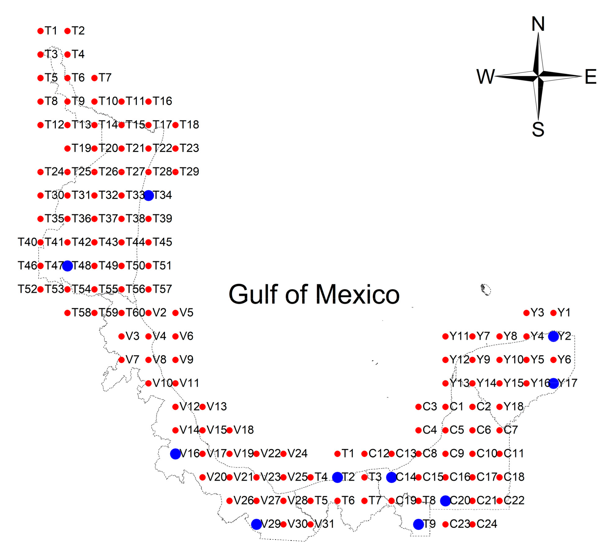
Mexico has five states along the Gulf of Mexico: Tamaulipas, Veracruz, Tabasco, Campeche, and Yucatan, as seen in Figure 1.

In order to carry out this study, data for 141 different sites along the Mexican Gulf were collected from the Modern-Era Retrospective Analysis for Research and Applications version 2 (MERRA-2) from the National Aeronautics and Space Administration (NASA); these are re-analysis data that are long-term, model-based analyses of multiple datasets using a fixed assimilation system [32]. MERRA-2 has presented data every hour from 1980 until 2017. According to Shang [33] the network measures derived from the empirical observations are often poor estimators of the true structure of system as it is impossible to observe all components and all interactions in many real-world complex systems. This problem occurs when there is missing data; in this study, MERRA-2 has no missing data; therefore, this problem is avoided and can be considered to be unbiased data.

In Figure 2, we give the geographic positions where MERRA-2 data were taken from.

2.2. The Weibull Distribution and Seasonal Wind

There are some statistical distribution functions for analyzing wind data, such as the lognormal, normal, Rayleigh, and Weibull probability distributions [34,35]. The Weibull function is the most-used function to assess wind energy potential because shows variables as shape and scale parameters [36], where these parameters are obtained using estimation methods, such as the maximum likelihood method, and the goodness of the resulting fits are evaluated using several indicators, e.g., the coefficient of determination (R²) [24,37,38,39]. The R² is a statistical measure that represents the proportion of the variance for a dependent variable that is explained by an independent variable; R² is generally interpreted as the percentage of a value’s movements that can be explained by movements of another variable [40].

2.2.1. Wind Model

The Weibull distribution and cumulative distribution functions are expressed in Equations (1) and (2), respectively [41]:

$$f\left(v\right) = \frac{k}{c}{\left(\frac{v}{c}\right)}^{k - 1}exp\left[-{\left(\frac{v}{c}\right)}^k\right]\left(k>0,v>0,c>1\right),$$

(1)

$$F\left(v\right) = 1 - exp\left[{\left(\frac{v}{c}\right)}^k\right],$$

(2)

where k is the shape parameter (dimensionless), which is considered a Weibull form parameter because it specifies the shape of the distribution taking place within values between 1 and 3. A small value for k signifies very variable winds, while constant winds are characterized by a larger k [42]; when the shape parameter is 2, it is considered to represent Rayleigh distribution. The scale parameter c has the same units as wind speed (m/s) and is proportional to the mean wind speed (v_m), where v (m/s) is the wind speed registered in the site.

If the mean wind speed in Equation (3), and the standard deviation (σ) are known, k and c can be calculated using Equations (4) and (5) as follows [43]:

$$v_m = \frac{1}{n}\left[{\displaystyle \sum }_{i = 1}^n{v}_i\right],$$

(3)

$$k = {\left(\frac{\sigma }{v_m}\right)}^{-1.086},$$

(4)

$$c = \frac{v_m}{\mathsf{\Gamma }\left(1 + \frac{1}{k}\right)}.$$

(5)

The gamma function, Γ, can be calculated using Equation (6):

$$\mathsf{\Gamma }\left(r\right) = {{\displaystyle \int }}_0^{\infty }{x}^{r - 1}{e}^{-x}dx.$$

(6)

2.2.2. Wind Power Analysis

The observed wind power density (WPD_O) can be obtained using Equation (7):

$$WP{D}_{O }= \frac{{{\displaystyle \sum }}_{i = 1}^{n}0.5\rho v_i^3}{n},$$

(7)

where ρ is the air density and is calculated using the ideal gas law (see Equation (8)), in which T is the absolute temperature (K), p is the absolute pressure (Pa), and R is the specific gas constant (J/kg∙K): As an approximation, R = 0.286 is used for dry air.

$$\rho = \frac{p}{RT}$$

(8)

2.3. Wind Variables Analysis

Calculations for wind variables were performed by implementing a self-written code on the R free software environment and language [44]. This environment, besides being free, provides powerful tools for statistical computing and graphical display via eight packages, and when required, they can be extended with additional packages available through the comprehensive R archive network (CRAN) family available on the Internet. In fact, in the former study, six base packages were used (tools, stats, graphics, grDevices, utils, and base) [44], which were complemented with the extra packages (lubridate [45], RColorBrewer [46], ggplot2 [47], and gridExtra [48]).

2.3.1. Data Processing

An iterative process was run for all 141 studied sites, which were distributed in a grid-shaped arrangement along the coast of the Gulf of Mexico (see Figure 2) using the previously mentioned MERRA-2 files as input data. These files contained complete time series data (no missing values) of the surface pressure (kPa), air temperature (°C) at 2 m and 10 m above ground level, wind speed (m/s) at 50 m above ground level, and wind direction (°) at 60 m above ground level; all these variables have hourly records from 1980 to 2016.

An annual and a seasonal analysis was performed for every site, where for the sake of simplicity, spring was considered to include the months of March, April, and May; summer included June, July, and August; autumn included September, October, and November; and Winter included December, January, and February.

The structure of the program consisted of an initial pre-processing of the MERRA-2 data, which generated an output file that was used for obtaining the geolocated values of the wind variables, as well as customized plots via two scripts named Weibull Analysis and Directional Analysis, as can be observed on Figure 3, and is explained as follows.

2.3.2. Pre-Processing

In the pre-processing step, a time adjustment was performed on the MERRA-2 data in order to assign the corresponding UTM zone (for Mexico −6 h) and make summertime corrections. Data was classified for years, months, days, and hours for further manipulation, and the air density and observed WPD were obtained via Equations (9) and (10), respectively.

Once the pre-processing was finished, an output was generated for feeding the following two independent and complementary scripts.

2.3.3. Weibull Analysis

The Weibull probability distribution function (PDF) and cumulative distribution function (CDF) were obtained and plotted according to Equations (1) and (2), respectively, for the annual and seasonal series.

Tables were generated with Weibull shapes and scale factors (k, c), mean wind speed (v_m), its corresponding standard deviation (σ), Weibull most-probable wind speed (v_mp), mean air density (ρ_m), and the observed wind power density (WPD_O).

2.3.4. Directional Analysis

In order to complement the Weibull distribution, a directional analysis was performed. For this, data was grouped according to the wind direction into 12 bins, corresponding to sectors as 30° segments. The cumulative WPD_O was obtained for every sector by considering the one with the highest value as the prevailing direction, which was obtained for complete years, as well as for every season.

2.4. Wind Clustering

The wind performance was grouped into several clusters using a k-means clustering model to identify its monthly behavior, which was analyzed to diagnose the time where the wind speed could be used to generated power. The k-means algorithm is widely used in data mining for the partitioning of n measured quantities into k clusters [49]; according to Sugar and James [50], the classification of observations into groups requires computing the distance between the observations [51,52,53,54]. The k-means algorithm is one of the simplest unsupervised machine learning algorithms, where unsupervised algorithms make inferences from datasets using only an input vector without referring to known, or labelled, outcomes [53]. We can define a cluster as a data set with similar characteristics. The k-means algorithm identifies k centroids and then allocates every data point to the nearest cluster [53]. This algorithm has been used in a study done by Wang et al. [55], where the k-means clustering algorithm was used to find the largest historical samples that had the greatest influence on forecasting accuracy to improve the efficiency of the proposed model.

A method for clustering was proposed by Deng et al. [52], which used a Weibull distribution to establish that an unclustered dataset P can be represented using Equation (9):

$$P = \left\{p_i, i = 1,2,3,\dots ,N^i\right\},$$

(9)

where p_i denotes the ith element and Nⁱ is the number of observations. The set of clusters C can be given as:

$$C = \left\{C_j|C_j\subset P, j = 1,2,3,\dots ,N^j\right\},$$

(10)

and the set of observations within a cluster, C_j, is represented by:

$$C_j = \left\{C_{jk}|C_{jk}\subset P, j = 1,2,3,\dots ,N^{jk}\right\}.$$

(11)

C_jk and N_jk are the kth observation with the jth cluster and the number of observations, respectively, in cluster set C_j. The set of centroids associated with the clusters W is given as:

$$W = \left\{W_j|W_j\subset C_j, j = 1,2,3,\dots ,N^j\right\},$$

(12)

where W_j is the jth centroid.

For wind clustering, each observation P is assigned to a cluster C_j and its centroid will be represented by its mean wind speed.

2.5. Wind Turbine Selection

The energy available for conversion mainly depends on the wind speed and the swept area of the wind turbine. Using Newton’s Law F = ma:

$$E = mas,$$

(13)

where E is the kinetic energy, m is the mass, a is the constant acceleration, and s is the distance. From kinematics, the acceleration can be expressed using Equation (14):

$$a = \frac{\left(v^2 - u^2\right)}{2s}.$$

(14)

Because the initial velocity of the object is 0, then u = 0, such that:

$$a = \frac{v^2}{2s}.$$

(15)

Substituting Equation (15) in Equation (13) gives:

$$E = \frac{1}{2}m{v}^2.$$

(16)

The rate of change of energy of the power in the wind is given by:

$$P = \frac{dE}{dt} = \frac{1}{2}{v}^2\frac{dm}{dt}.$$

(17)

The mass flow rate is expressed as:

$$\frac{dm}{dt} = \rho A\frac{dx}{dt},$$

(18)

and the distance’s rate of change is:

$$\frac{dx}{dt} = v.$$

(19)

Substituting Equation (18) into Equation (19) gives:

$$\frac{dm}{dt} = \rho Av.$$

(20)

Hence, from Equation (17), the wind power output generated by a wind turbine can be expressed using Equation (21):

$$P_{WT} = \frac{1}{2}\rho A{U}^3,$$

(21)

where P_WT is the rated power, ρ is the air density, A is the rotor area, and U is the wind speed approaching the turbine. According to Grillo et al. [56], the power coefficient is a function of the tip speed ratio, known as lambda (λ), and the blade pitch angle (β) (°). λ can be calculated Equation (22):

$$\lambda = \frac{\omega R}{U},$$

(22)

where ω is the rotational speed of the rotor (rad/s) and R is the rotor radius (m).

To characterize the wind speed in this study, a proposal for wind turbine selection is given, where this proposal considers the air density, rotor area, wind turbine power curve, and power coefficient (C_p).

Song et al. [57] defined the power coefficient C_p as the ratio of the power extracted from the wind turbine to the available power. C_p can be calculated as follows:

$$C_p = \frac{P_n}{\frac{1}{2}\rho A{u}_j^3}.$$

(23)

The C_p of a wind turbine is a measurement of how efficiently the wind turbine converts the energy in the wind into electricity.

Wind speed is one of the most important parameters in determining the electric power, and the general equation is related to the density of air, wind speed, and swept area, as in Equation (21), and represents the total energy obtained from the wind resource; however, in terms of generating electricity, only a certain proportion of energy can be converted and is expressed by Equation (24), as follows:

$$P_e = {\eta }_e{\eta }_m{C}_p{P}_{wT},$$

(24)

where P_e is the amount of electric power generated, η_e is the electrical conversion efficiency of the wind turbine, and η_m is the mechanical efficiency [58].

There is an optimization proposal that uses the wind turbine efficiency as a fundamental variable to determine the power output generated by a wind power farm [59]. In this proposal, as in this study to determine it, a Weibull distribution was used. The parameter c from the Weibull distribution was used to select a wind turbine according to its C_p; in this case, the maximum efficiency of a wind turbine was compared to the parameter c calculated from the wind speed site studied.

3. Results and Discussion

The annual Weibull parameters c and k, WPD_F, WPD_O, ρ, v_m, v_mp, and v_maxE were obtained for the 141 MERRA-2 data locations.

Table 1. MERRA-2 analysis.

State	ID	c	k	WPDO	ρ	vm	vmp
		(m/s)	(–)	(W/m2)	(kg/m3)	(m/s)	(m/s)
Tamaulipas	Tam34	8.26	2.71	357.09	1.19	7.34	6.97
Tamaulipas	Tam48	4.18	2.27	48.32	1.10	3.71	3.24
Veracruz	Ver16	3.86	2.23	37.82	1.06	3.42	2.96
Veracruz	Ver29	6.46	2.40	182.18	1.17	5.72	5.16
Tabasco	Tab2	6.90	2.84	200.40	1.18	6.15	5.93
Tabasco	Tab9	4.02	2.76	40.02	1.17	3.58	3.42
Campeche	Cam14	6.51	3.08	161.68	1.18	5.82	5.73
Campeche	Cam20	2.90	3.04	14.14	1.17	2.59	2.54
Yucatan	Yuc2	5.10	3.07	79.38	1.19	4.56	4.48
Yucatan	Yuc17	2.99	3.10	15.76	1.18	2.67	2.63

only presents the places with the highest and lowest mean wind speeds for each state (colored blue in Figure 2); these values were used as references for the seasonal analysis.

Tamaulipas was the state with more zones with high values of wind than the other states, where its maximum v_m = 7.34 m/s, scale and shape parameters were between 4.17–8.26 m/s and 1.97–2.91, respectively. In this case, by comparing v_m, c, and k, it can be established that in the time domain, most of the wind resource had values higher than its mean wind speed. In Veracruz, the scale and shape parameters showed values between 3.86–6.88 m/s and 1.72–2.41, respectively. Tabasco presented more wind speed and wind resource than Veracruz with Weibull parameters ranging between 4.02–7.48 m/s for c, and 2.51–3.07 for k. Campeche and Yucatan showed a higher k’s than the others states, with 2.71 and 2.95, respectively, which can be interpreted as a long period of time with winds higher than their means; c was 7.47 m/s and 7.88 m/s for Campeche and Yucatan, respectively.

According to Katinas et al. [29], the Weibull parameter c has the same behavior as the WPD, where in all cases, when the scale factor grows, the WPD grows as well. It is important to mention that the lowest shape parameter corresponds to the lowest wind speed, which means that the frequency of data below the mean was greater than that above it.

3.1. Seasonal Weibull Parameters and WPD

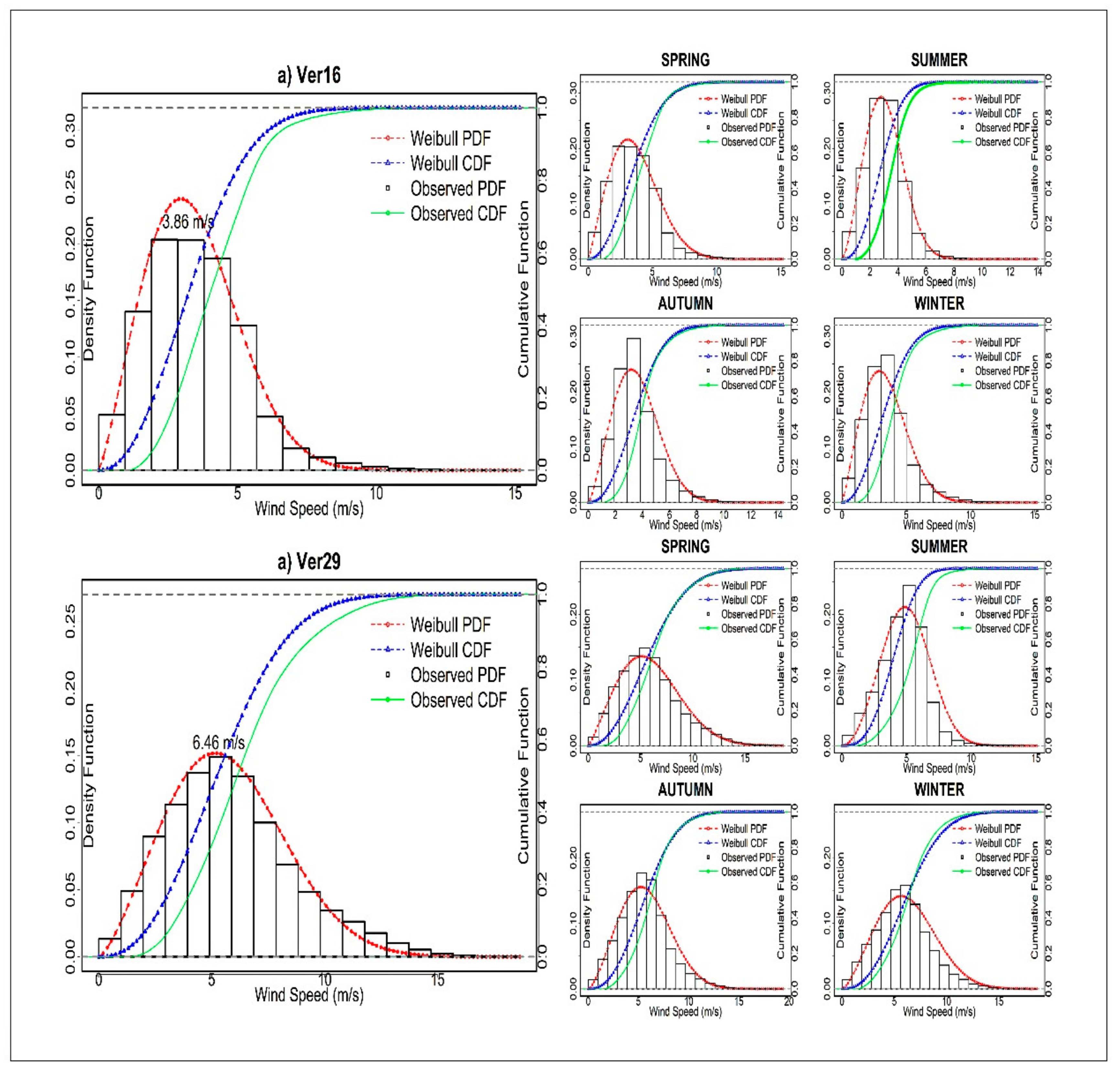
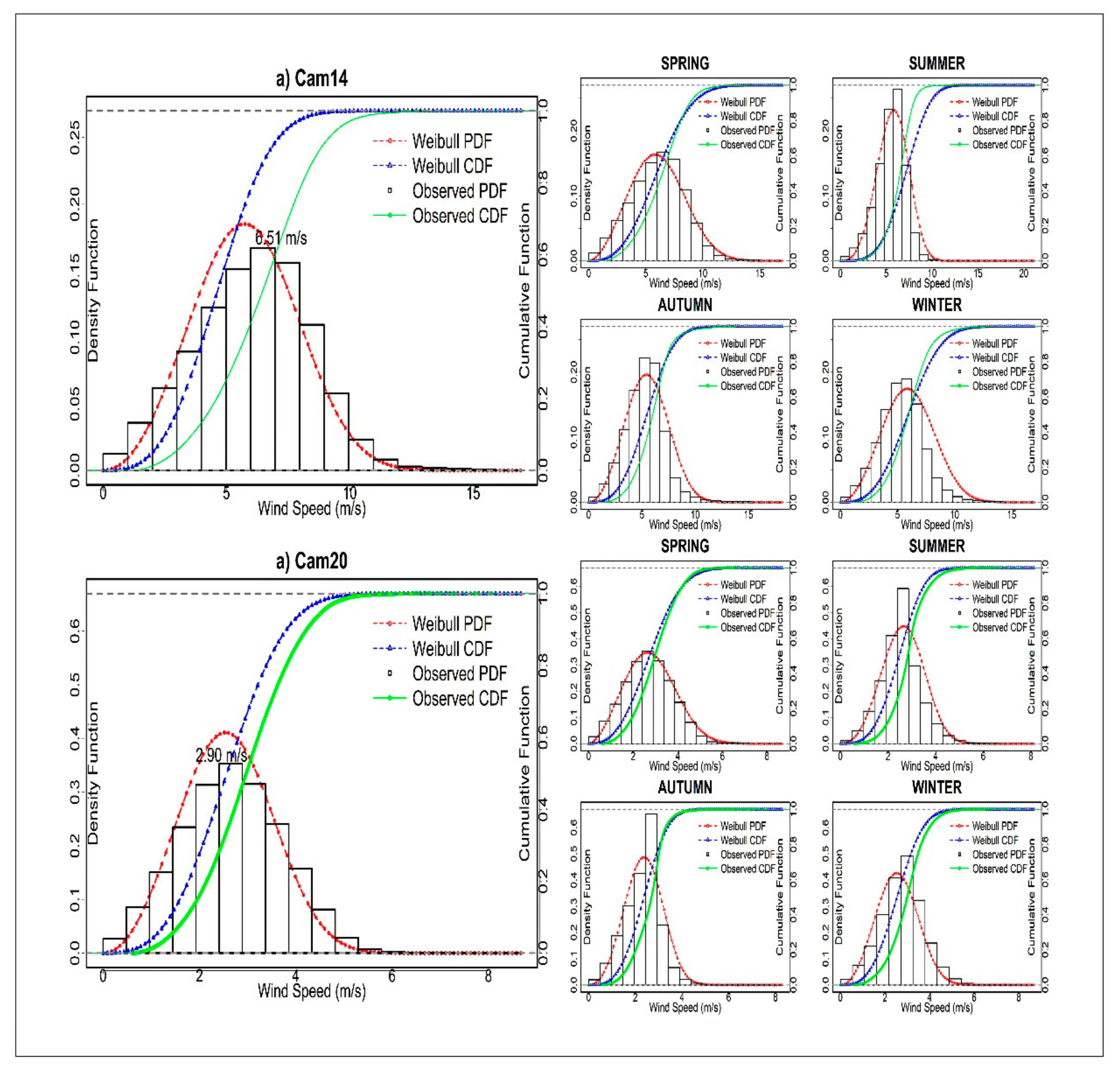
Seasonal wind speed characterization was carried out by dividing the data according to the four annual seasons: spring (March, April, and May); summer (June, July, and August); autumn (September, October and November); and winter (December, January and February). For the sake of analysis, two sites for each state were chosen by considering its highest and lowest mean wind speed (see Figure 4, Figure 5, Figure 6, Figure 7 and Figure 8).

In Figure 4, it can be observed that the points Tam34 and Tam48 had the highest and the lowest mean wind speed—8.26 m/s and 4.18 m/s, respectively—in the state of Tamaulipas. At the annual level, Tam34 had k = 2.71, which represents a very good value due its higher magnitudes of wind speed; at the seasonal level, the Weibull distribution shows that spring and winter are the periods of time during an average year where there was more available wind resource.

In the state of Veracruz, 31 locations were studied, with the highest scale parameter being found for Ver29, where this was located is in the Isthmus of Tehuantepec, one of the windiest zones in the world. During an average year, its highest mean wind speed was 5.72 m/s, its c was 6.46 m/s, and k was 2.40, and had a windy season during spring, autumn, and winter (see Figure 5).

In Tabasco (Figure 6), Tab2 had c = 6.90 m/s, k = 2.84, and a mean wind speed of 6.15 m/s; these values represent a good wind resource because analyzing Weibull parameters showed that c was higher than its mean, and k showed that most of the time, the wind speed data was above its mean. In contrast, the seasonal Weibull of Tab9, which was the point with the lowest values in this state (c = 4.02 m/s, k = 2.76, v_m = 3.58 m/s), allowed to determine a period of wind during an average year that had constant magnitudes of wind values, namely winter, spring, and summer, as shown.

The analysis of Campeche (Figure 7) showed its windiest location was Cam14, which had a mean wind speed of 5.82 m/s, and c and k values equal to 6.51 m/s and 3.08, respectively. The lowest valued location, Cam20, had c = 2.90 m/s and v_m = 2.64 m/s, where both values are similar with a difference of 0.26 m/s, which can be considered as a location that did not have variations during an average year. Its k = 3.04 could be considered a very good frequency of wind speed; however, due its low wind speed, it did not represent an impactful wind resource, which can be seen in the seasonal analysis because its variation was minimal.

In Yucatan, as seen in Figure 8, its seasonal wind variation was divided in two periods, highest one between winter and spring and the lowest one between summer and autumn. The location with the highest wind speed was Yuc2 (v_m = 4.56 m/s, c = 5.10 m/s, and k = 3.07), and the lowest location, Yuc17, was inside a rainforest, which reduced the magnitude of the wind speed (v_m = 2.67 m/s, c = 2.99, and k = 3.10).

These results are in agreement with the study developed by Herrero-Novoa [30], where it was established that dividing an average year into two periods (spring–summer and fall–winter) provides more accuracy regarding wind characterization; in a similar fashion, for the current study, an average year was divided into four periods of time (seasons) where even more accurate wind periods were established. This allowed us to determine the wind characteristics, specifically its WPD, in the most relevant period. By observing Figure 8 and considering the values of the parameters obtained in Table 1, we established that in Yuc2, the parameter c = 5.10 m/s was higher than its average of 4.56 m/s, and its k = 3.07; therefore, at this site, the wind speed was over 4.56 m/s most of the time. Furthermore, according to Vazquez et al. [42], this value of k means that the site had constant winds.

In addition to the Weibull analysis, in Figure 9 and Figure 10, the prevailing wind directions and the magnitude of its WPD_O can be observed for the annual and seasonal behavior, respectively.

The highest WPD_O points were along Tamaulipas and Veracruz, although Tamaulipas had more locations than Veracruz, while Veracruz has the highest resource next to the sea, Tamaulipas had it at the border with the United States of America.

As can be observed in Figure 10, the seasons with greatest WPD_O were autumn and winter, and the states with greatest resource were Tamaulipas and Veracruz. Regarding wind orientation, this figure shows that Tamaulipas had two periods with different prevailing directions, with the first one during spring and summer and the second one in autumn and winter. The WPD in southern Veracruz presented the same direction most of the time (southeast), meanwhile Tabasco, which is the southernmost state along the Gulf of Mexico, had different prevailing orientations throughout an average year. It can also be seen that Campeche had a prevailing direction in winter and spring, and for Yucatan, autumn, winter, and spring had northeast as the predominant direction, while it was southeast in summer.

3.2. Wind Speed and Wind Power Clustering

Using k-means clustering, the wind speed could be clustered into months, and in these clusters, the power output could be calculated. Figure 11 shows the clustering done for wind speed from 1980–2017.

Wind speed was divided into three clusters—C₁, C₂, and C₃—as shown in Figure 11 where the blocks represent the amount of wind speed each month.

Taking these results and knowing the windy seasons throughout an average year, the wind power output could be calculated. A critical point in this stage was to select the wind turbine, where in

Table 2. Wind turbine C_p.

Wind Turbine	Cp	Wind Speed (m/s) @ Cp
Acciona AW70/1500 Class III	0.4188	6.5
Acciona AW70/1500 Class II	0.4457	7.5
Ecotecnia 48	0.4142	8.5
Clipper Liberty C93	0.4215	9.5
Nordex S70 1500 kW	0.4410	10
Vestas V90 1.8 MW	0.4381	8

, we present the C_p of different wind turbines as a first step to know the efficiency of each one of them. The wind turbines were selected according to parameter c of the points analyzed.

Six wind turbines were found such that their C_p fit with the parameter c calculated from the wind speed data.

Table 3. Wind turbine selection.

ID Point	c (m/s)	Cp	Wind Turbine	ηe (%)	ηm (%)	Probable Energy Production (kWh)
Cam14	6.51	0.4188	Acciona AW70/1500 III	39	96	1,089,556.34
Cam4	6.65	0.4188	Acciona AW70/1500 III	39	96	870,467.93
Cam13	7.15	0.4457	Acciona AW70/1500	39	96	880,222.72
Cam3	7.39	0.4457	Acciona AW70/1500	39	96	1,266,250.78
Cam12	7.47	0.4457	Acciona AW70/1500	39	96	1,330,923.23
Tab3	6.70	0.4188	Acciona AW70/1500 III	39	96	901,712.57
Tab2	6.90	0.4188	Acciona AW70/1500 III	39	96	975,917.27
Tab4	6.96	0.4188	Acciona AW70/1500 III	39	96	995,083.68
Tab1	7.48	0.4457	Acciona AW70/1500	39	96	1,324,954.98
Tam44	6.67	0.4188	Acciona AW70/1500 III	39	96	874,886.55
Tam5	6.72	0.4188	Acciona AW70/1500 III	39	96	892,710.52
Tam57	6.74	0.4188	Acciona AW70/1500 III	39	96	892,710.52
Tam19	6.75	0.4188	Acciona AW70/1500 III	39	96	901,712.57
Tam38	6.81	0.4188	Acciona AW70/1500 III	39	96	933,696.07
Tam32	6.94	0.4188	Acciona AW70/1500 III	39	96	985,469.41
Tam51	6.99	0.4188	Acciona AW70/1500 III	39	96	995,083.68
Tam1	7.01	0.4457	Acciona AW70/1500	39	96	1,084,869.22
Tam13	7.13	0.4457	Acciona AW70/1500	39	96	1,132,490.97
Tam3	7.13	0.4457	Acciona AW70/1500	39	96	1,137,866.71
Tam2	7.17	0.4457	Acciona AW70/1500	39	96	1,159,539.79
Tam9	7.33	0.4457	Acciona AW70/1500	39	96	1,231,874.84
Tam33	7.42	0.4457	Acciona AW70/1500	39	96	1,289,519.75
Tam6	7.44	0.4457	Acciona AW70/1500	39	96	1,295,381.19
Tam4	7.46	0.4457	Acciona AW70/1500	39	96	1,313,072.04
Tam11	7.51	0.4457	Acciona AW70/1500	39	96	1,342,913.46
Tam10	7.52	0.4457	Acciona AW70/1500	39	96	1,348,935.48
Tam7	7.52	0.4457	Acciona AW70/1500	39	96	1,348,935.48
Tam45	7.61	0.4457	Acciona AW70/1500	39	96	1,379,315.79
Tam15	7.65	0.4457	Acciona AW70/1500	39	96	1,416,370.08
Tam26	7.65	0.4457	Acciona AW70/1500	39	96	1,403,945.85
Tam20	7.67	0.4457	Acciona AW70/1500	39	96	1,422,609.58
Tam14	7.68	0.4457	Acciona AW70/1500	39	96	1,428,867.39
Tam21	7.77	0.4382	Vestas v90 1.8 MW	39.7	96.1	2,404,698.21
Tam27	7.79	0.4382	Vestas v90 1.8 MW	39.7	96.1	2,425,608.51
Tam17	7.84	0.4382	Vestas v90 1.8 MW	39.7	96.1	2,478,413.83
Tam16	7.85	0.4382	Vestas v90 1.8 MW	39.7	96.1	2,489,066.02
Tam22	8.07	0.4382	Vestas v90 1.8 MW	39.7	96.1	2,697,298.23
Tam29	8.08	0.4382	Vestas v90 1.8 MW	39.7	96.1	2,686,059.50
Tam39	8.08	0.4382	Vestas v90 1.8 MW	39.7	96.1	2,686,059.50
Tam23	8.14	0.4382	Vestas v90 1.8 MW	39.7	96.1	2,765,389.54
Tam28	8.20	0.4382	Vestas v90 1.8 MW	39.7	96.1	2,822,999.99
Tam18	8.21	0.4382	Vestas v90 1.8 MW	39.7	96.1	2,834,617.26
Tam34	8.26	0.4382	Vestas v90 1.8 MW	39.7	96.1	2,869,660.21
Ver2	6.46	0.4188	Acciona AW70/1500 III	39	96	345,346.79
Ver29	6.46	0.4188	Acciona AW70/1500 III	39	96	785,191.78
Ver22	6.47	0.4188	Acciona AW70/1500 III	39	96	789,317.12
Ver13	6.60	0.4188	Acciona AW70/1500 III	39	96	844,268.34
Ver25	6.64	0.4188	Acciona AW70/1500 III	39	96	857,301.42
Ver9	6.74	0.4188	Acciona AW70/1500 III	39	96	892,710.52
Ver5	6.82	0.4188	Acciona AW70/1500 III	39	96	924,482.03
Ver6	6.83	0.4188	Acciona AW70/1500 III	39	96	929,081.43
Ver24	6.88	0.4188	Acciona AW70/1500 III	39	96	952,307.41
Yuc13	6.64	0.4188	Acciona AW70/1500 III	39	96	870,467.93
Yuc7	7.27	0.4457	Acciona AW70/1500	39	96	1,231,874.84
Yuc12	7.28	0.4457	Acciona AW70/1500	39	96	1,231,874.84
Yuc3	7.44	0.4457	Acciona AW70/1500	39	96	1,319,004.59
Yuc1	7.54	0.4457	Acciona AW70/1500	39	96	1,373,203.61
Yuc11	7.88	0.4382	Vestas V90 1.8 MW	39	96	1,531,691.62

presents the wind turbine selected for each point along the Gulf of Mexico.

A total of 58 points were fitted with an appropriate wind turbine C_p, where the wind speed of the site was related to the wind speed at the maximum wind turbine efficiency; with this information, the best option for the wind turbine to be used could be determined based on its C_p. The probable energy production was calculated for each wind turbine selected using Equation (16) based on the electrical and mechanical efficiency given by the manufacturer.

4. Conclusions

The seasonal characterization of wind speeds along the Mexican states of the Gulf of Mexico was done for 141 locations with MERRA-2 data, with records between 1980–2017. An average year of wind data for each location was obtained and these were divided according to the seasons of the year (spring, summer, autumn, and winter). This distinction allowed us to describe the wind characteristics more accurately, especially the WPD, which allowed for establishing wind seasons properly, as well as the description of the prevailing wind direction. It is was found that there were different wind seasons along the states of the Gulf of Mexico and they were established for each state. The wind season in Tamaulipas occurred in winter and spring; Veracruz and Tabasco had a wind season in autumn, winter, and spring; and in Campeche and Yucatan, the wind season was in winter and spring, where these states shared their coast with both the Gulf of Mexico and the Caribbean Sea. This variation allowed us to determine that the wind season could depend upon other factors regarding the climatology of each state.

The state with the greatest wind resource was Tamaulipas, as seen in Figure 9; it had plenty of locations with good values for wind, scale, and shape parameters, where its highest v_m, c, and k was 7.34 m/s, 8.26 m/s, and 2.91 respectively. North and south Veracruz had the highest values of wind speed, where its southern zone corresponded to the Isthmus of Tehuantepec, one of the zones with the greatest wind energy resource in the world; its highest parameters were v_m = 6.10 m/s, c = 6.88 m/s, and k = 2.41. Tabasco presented the following parameters: v_m = 6.67 m/s, c = 7.48 m/s, and k = 3.07. These three states (Tamaulipas, Veracruz, and Tabasco) presented the same wind season.

The highest parameters for Campeche were v_m = 6.57 m/s, c = 7.39 m/s, and k = 2.71, and the Yucatan parameters were v_m = 7.88 m/s, c = 7.04 m/s, and k = 3.07; these two states presented the same wind season.

Three clusters were found, which were useful for determining the wind speed in monthly groups and to visualize the wind stations in the study area of the Gulf of Mexico.

Using C_p, optimal wind turbines were determined by comparing it with the parameter c of Weibull distribution. In this study, 58 sites were fitted with a wind turbine C_p, and by analyzing these data, three wind turbines were selected: Acciona AW70/1500 Class III with a C_p = 0.4188 at 6.5 m/s, Acciona AW70/1500 Class II with a C_p = 0.4457 at 7.5 m/s, and Vestas V90 1.8 MW with a C_p = 0.4381 at 8 m/s.

At the end of this study, the probable energy production was calculated for each wind turbine applied at each site with its own respective conditions.

Regarding future research lines, we propose following the proposal to select the most efficient wind turbine by adding more constraints, such as wind direction, roughness, and orography.

References

- IEA. International Energy Agency. 2019. Available online: https://www.iea.org/ (accessed on 14 October 2019).
- IRENA. International Renewable Energy Agency. 2019. Available online: https://www.irena.org/ (accessed on 15 October 2019).
- IEA. Renewables, International Energy Agency Renewables. 2018. Available online: https://www.iea.org/renewables (accessed on 24 October 2018).
- Davis, R.E.; Kalkstein, L. Development of an automated spatial synoptic climatological classification. Int. J. Clim. 1990, 10, 769–794. [Google Scholar] [CrossRef]
- Montoya, F.G.; Manzano-Agugliaro, F.; López-Márquez, S.; Hernández-Escobedo, Q.; Gil, C. Wind turbine selection for wind farm layout using multi-objective evolutionary algorithms. Expert Syst. Appl. 2014, 41, 6585–6595. [Google Scholar] [CrossRef]
- Ley de Transición Energética, LTE. 2015. Available online: http://www.diputados.gob.mx/LeyesBiblio/pdf/LTE.pdf. (accessed on 22 October 2018).
- SIE. Sistema de Información Energética. 2019. Available online: http://sie.energia.gob.mx/bdiController.do?action=cuadro&cvecua=IE0C01 (accessed on 14 October 2019).
- Bandi, M.M.; Apt, J. Variability of the Wind Turbine Power Curve. Appl. Sci. 2016, 6, 262. [Google Scholar] [CrossRef] [Green Version]
- Hernandez-Escobedo, Q. Wind Energy Assessment for Small Urban Communities in the Baja California Peninsula, Mexico. Energies 2016, 9, 805. [Google Scholar] [CrossRef]
- Avila-Calero, S. Contesting energy transitions: Wind power and conflicts in the Isthmus of Tehuantepec. J. Polit. Ecol. 2017, 24, 992–1012. [Google Scholar] [CrossRef] [Green Version]
- Ospino-Castro, A.; Pena-Gallardo, R.; Hernandez-Rodriguez, A.; Segundo-Ramirez, J.; Munoz-Maldonado, Y.A. Techno-economic evaluation of a grid-connected hybrid PV-Wind power generation system in San Luis Potosi, Mexico. In Proceedings of the 2017 IEEE International Autumn Meeting on Power, Electronics and Computing (ROPEC), Ixtapa, Mexico, 8–10 November 2017. [Google Scholar]
- Santamaria-Bonfil, G.; Reyes-Ballesteros, A.; Gershenson, C. Wind speed forecasting for wind farms: A method based on support vector regression. Renew. Energy 2016, 85, 790–809. [Google Scholar] [CrossRef]
- Hernandez-Escobedo, Q.; Manzano-Agugliaro, F.; Zapata-Sierra, A. The wind power of Mexico. Renew. Sustain. Energy Rev. 2010, 14, 2830–2840. [Google Scholar] [CrossRef]
- Mazzeo, D.; Oliveti, G.; Labonia, E. Estimation of wind speed probability density function using a mixture of two truncated normal distributions. Renew. Energy 2018, 115, 1260–1280. [Google Scholar] [CrossRef]
- Gugliani, G.K.; Sarkar, A.; Ley, C.; Mandal, S. New methods to assess wind resources in terms of wind speed, load, power and direction. Renew. Energy 2018, 129, 168–182. [Google Scholar] [CrossRef]
- Green, M.C.; Myrup, L.O.; Flocchini, R.G. A method for classification of wind field patterns and its application to southern California. Int. J. Climatol. 1992, 12, 111–135. [Google Scholar] [CrossRef]
- Jimenez, P.A.; Gonzalez-Rouco, J.F.; Montavez, J.P.; Navarro, J.; Garcia-Bustamante, E.; Valero, F. Surface wind regionalization in complex terrain. J. Appl. Meteorol. Climatol. 2008, 47, 308–325. [Google Scholar] [CrossRef] [Green Version]
- Hernandez-Escobedo, Q.; Manzano-Agugliaro, F.; Gazquez-Parra, J.A.; Zapata-Sierra, A. Is the wind a periodical phenomenon? The case of Mexico. Renew. Sustain. Energy Rev. 2011, 15, 721–728. [Google Scholar] [CrossRef]
- Jimenez, P.A.; Gonzalez-Rouco, J.F.; Garcia-Bustamante, E.; Navarro, J.; Montavez, J.P.; Valero, F.; Arellano, J.V.; Dudhia, J.; Munoz-Roldan, A. Surface wind regionalization over complex terrain: Evaluation and analysis of a high-resolution WRF simulation. J. Appl. Meteorol. Climatol. 2010, 49, 268–287. [Google Scholar] [CrossRef] [Green Version]
- Zapata-Sierra, A.J.; Cama-Pinto, A.; Montoya, F.G.; Alcayde, A.; Manzano-Agugliaro, F. Wind missing data arrangement using wavelet based techniques for getting maximum likelihood. Energy Convers. Manag. 2019, 185, 552–561. [Google Scholar] [CrossRef]
- Kaufmann, P.; Whiteman, C.D. Cluster-Analysis Classification of wintertime wind patterns in the Grand Canyon region. J. Appl. Meteorol. 1999, 38, 1131–1147. [Google Scholar] [CrossRef]
- Jinsol, K.; Hyun-Goo, K.; Hyeong-Dong, P. Surface Wind Regionalization Based on Similarity of Time-series Wind Vectors. Asian J. Atmos. Environ. 2016, 10, 80–89. [Google Scholar]
- Weber, R.O.; Kaufmann, P. Automated classification scheme for wind fields. J. Appl. Meteorol. 1995, 34, 1133–1141. [Google Scholar] [CrossRef]
- Saleh, H.; Abou El-Azm Aly, A.; Abdel-Hady, S. Assessment of different methods used to estimate Weibull distribution parameters for wind speed in Zafarana wind farm, Suez Gulf, Egypt. Energy 2012, 44, 710–719. [Google Scholar] [CrossRef]
- Aukitino, T.; Khan, M.G.M.; Ahmed, M.R. Wind energy resource assessment for Kiribati with a comparison of different methods of determining Weibull parameters. Energy Convers. Manag. 2017, 151, 641–660. [Google Scholar] [CrossRef]
- Akdağ, S.A.; Dinler, A. A new method to estimate Weibull parameters for wind energy applications. Energy Convers. Manag. 2009, 50, 1761–1766. [Google Scholar] [CrossRef]
- Baseer, M.A.; Meyer, J.P.; Rehman, S.; Alam, M.M. Wind power characteristics of seven data collection sites in Jubail, Saudi Arabia using Weibull parameters. Renew. Energy 2017, 102, 35–49. [Google Scholar] [CrossRef] [Green Version]
- Ozay, C.; Celiktas, M.S. Statistical analysis of wind speed using two-parameter Weibull distribution in Alaçatı region. Energy Convers. Manag. 2016, 121, 49–54. [Google Scholar] [CrossRef]
- Katinas, V.; Gecevicius, G.; Marciukaitis, M. An investigation of wind power density distribution at location with low and high wind speeds using statistical model. Appl. Energy 2018, 218, 442–451. [Google Scholar] [CrossRef]
- Herrero-Novoa, C.; Pérez, I.A.; Sánchez, M.L.; García, M.Á.; Pardo, N.; Fernández-Duque, B. Wind speed description and power density in northern Spain. Energy 2017, 138, 967–976. [Google Scholar] [CrossRef] [Green Version]
- Faghani, G.H.R.; Ashrafi, Z.N.; Sedaghat, A. Extrapolating wind data at high altitudes with high precision methods for accurate evaluation of wind power density, case study: Center of Iran. Energy Convers. Manag. 2018, 157, 317–338. [Google Scholar] [CrossRef]
- MERRA. Modern-Era Retrospective Analysis for Research and Applications (MERRA). 2018. Available online: https://gmao.gsfc.nasa.gov/reanalysis/MERRA/ (accessed on 10 August 2018).
- Shang, Y. Subgraph Robustness of Complex Networks under Attacks. IEEE Trans. Syst. Man Cybern. Syst. 2019, 49, 821–832. [Google Scholar] [CrossRef]
- Fagbenle, R.O.; Katende, J.; Ajayi, O.O.; Okeniyi, J.O. Assessment of wind energy potential of two sites in North-East, Nigeria. Renew. Energy 2011, 36, 1277–1283. [Google Scholar] [CrossRef]
- Ozerdem, B.; Turkeli, M. An investigation of wind characteristics on the campus of Izmir Institute of Technology, Turkey. Renew. Energy 2003, 28, 1013–1027. [Google Scholar] [CrossRef] [Green Version]
- Hocaoğlu, F.O.; Fidan, M.; Gerek, Ö.N. Mycielski approach for wind speed prediction. Energy Convers. Manag. 2009, 50, 1436–1443. [Google Scholar] [CrossRef]
- Carta, J.A.; Ramírez, P.; Velázquez, S. A review of wind speed probability distributions used in wind energy analysis: Case studies in the Canary Islands. Renew. Sustain. Energy Rev. 2009, 13, 933–955. [Google Scholar] [CrossRef]
- Celik, A. Assessing the suitability of wind speed probability distribution functions on wind power density. Renew. Energy 2003, 28, 1563–1574. [Google Scholar] [CrossRef]
- Seguro, J.V.; Lambert, T.W. Modern estimation of the parameters of the Weibull wind speed distribution for wind energy analysis. J. Wind Eng. Ind. Aerodyn. 2000, 85, 75–84. [Google Scholar] [CrossRef]
- Montgomery, D. Introduction to Statistical Quality Control, 6th ed.; John Wiley and Sons: Hoboken, NJ, USA, 2009. [Google Scholar]
- Montgomery, D.; Runger, G. Applied Statistics and Probability for Engineers, 3rd ed.; John Wiley and Sons: Hoboken, NJ, USA, 2003. [Google Scholar]
- Vasquez, A.; Sousa, T. Stability Analysis of Distribution Networks using The Cespedes Load Flow Considering Wind Energy Conversion Systems. In Proceedings of the 2018 IEEE PES Transmission & Distribution Conference and Exhibition Latin America, Lima, Perú, 18–21 September 2018. [Google Scholar]
- Bilir, L.; İmir, M.; Devrim, Y.; Albostan, A. Seasonal and yearly wind speed distribution and wind power density analysis based on Weibull distribution function. Int. J. Hydrog. Energy 2015, 40, 15301–15310. [Google Scholar] [CrossRef]
- R Core Team. R: A Language and Environment for Statistical Computing. R Foundation for Statistical Computing: Vienna, Austria, 2018. Available online: https://www.R-project.org/ (accessed on 2 January 2019).
- Grolemund, G.; Wickham, H. Dates and Times Made Easy with lubridate. J. Stat. Softw. 2011, 40, 1–25. [Google Scholar] [CrossRef]
- Neuwirth, E. RColorBrewer: ColorBrewer Palettes. R Package Version 1.1-2. 2014. Available online: https://rdrr.io/cran/RColorBrewer/ (accessed on 3 January 2019).
- Wickham, H. ggplot2: Elegant Graphics for Data Analysis, First; Springer: New York, NY, USA, 2016. [Google Scholar]
- R Project. 2019. Available online: https://cran.r-project.org/web/packages/gridExtra/index.html (accessed on 3 January 2019).
- Kassambara, A. Practical Guide to Cluster Analysis in R, 1st ed.; STHDA: Scotts Valley, CA, USA, 2017; Available online: https://www.datanovia.com/en/wp-content/uploads/dn-tutorials/book-preview/clustering_en_preview.pdf (accessed on 25 March 2019).
- Sugar, C.A.; James, G.M. Finding the number of clusters in data set: An information theoretic approach. J. Am. Stat. Assoc. 2003, 98, 750–763. [Google Scholar] [CrossRef]
- Hao, Y.; Dong, L.; Liao, X.; Liang, J.; Wang, L.; Wang, B. A novel clustering algorithm based on mathematical morphology for wind power generation prediction. Renew. Energy 2019, 136, 572–585. [Google Scholar] [CrossRef]
- Zhu, X.; Liu, W.; Zhang, J. Probabilistic load flow method considering large-scale wind power integration. J. Mod. Power Syst. Clean Energy 2019, 7, 813–825. [Google Scholar]
- van Vuuren, C.Y.J.; Vermeulen, H.J. Wind resource clustering based on statistical Weibull characteristics. Wind Eng. 2019, 43, 359–376. [Google Scholar] [CrossRef]
- Demšar, J.; Curk, T.; Erjavec, A.; Gorup, Č.; Hočevar, T.; Milutinovič, M.; Štajdohar, M. Orange: Data Mining Toolbox in Python. J. Mach. Learn. Res. 2013, 14, 2349–2353. [Google Scholar]
- Wang, K.; Qi, X.; Liu, H.; Song, J. Deep belief network based k-means cluster approach for short-term wind power forecasting. Energy 2018, 165, 840–852. [Google Scholar] [CrossRef]
- Wind Turbines Integration with Storage Devices: Modelling and Control Strategies. Available online: https://www.researchgate.net/publication/221911678_Wind_Turbines_Integration_with_Storage_Devices_Modelling_and_Control_Strategies/link/0deec521b17b05c5ba000000/download (accessed on 1 December 2019).
- Song, D.; Liu, J.; Yang, J.; Su, M.; Yang, S.; Yang, X.; Joo, Y.H. Multi-objective energy-cost design optimization for variable-speed wind turbine at high-altitude sites. Energy Convers. Manag. 2019, 196, 513–524. [Google Scholar] [CrossRef]
- Elsevier. Wind Energy a Handbook for Onshore and Offshore Wind Turbines; Academic Press: Cambridge, MA, USA, 2017; ISBN 978-0-12-809451-8. [Google Scholar]
- Ouammi, A.; Dagdougui, H.; Sacile, R. Optimal Planning with Technology Selection for Wind Power Plants in Power Distribution Networks. IEEE Syst. J. 2019, 13, 3059–3069. [Google Scholar] [CrossRef]
Figure 1.
Mexican states along the Gulf of Mexico.
Figure 2.
Modern-Era Retrospective Analysis for Research and Applications version 2 (MERRA-2) data locations.
Figure 3.
Program structure. CDF: cumulative density function, PDF: probability distribution function.
Figure 4.
Annual and seasonal Weibull distributions in the state of Tamaulipas.
Figure 5.
Annual and seasonal Weibull distributions for the state of Veracruz.
Figure 6.
Annual and seasonal Weibull distributions for the state of Tabasco.
Figure 7.
Annual and seasonal Weibull distributions for the state of Campeche.
Figure 8.
Annual and seasonal Weibull distributions for the state of Yucatan.
Figure 9.
Annual prevailing wind direction and its WPDO along the states of the Gulf of Mexico.
Figure 10.
Seasonal prevailing wind direction and its WPDO along the states of the Gulf of Mexico.
Figure 11.
Wind speed clustering in the Mexican states of the Gulf of Mexico.