Impact of Building Orientation on Daylight Availability and Energy Savings Potential in an Academic Classroom

Faculty of Environmental Engineering and Energy, Poznan University of Technology, ul. Piotrowo 3a, 60-965 Poznań, Poland
Energies 2020, 13(18), 4916; https://0-doi-org.brum.beds.ac.uk/10.3390/en13184916
Submission received: 18 August 2020
/
Revised: 16 September 2020
/
Accepted: 17 September 2020
/
Published: 19 September 2020
(This article belongs to the Special Issue Smart Built Environment for Health and Comfort with Energy Efficiency)
Abstract
:In this paper, daylight availability depending on building orientation in a typical educational classroom was investigated. Measurements of daylight illuminance distributions in the room depth for different illuminance outside the building allowed to determine the conditions when the luminaires in a classroom could be turned off, turned on, or dimmed. The outdoor daylight illuminance on the south-east and north façade of the building was recorded and the numbers of hours per year of university activity during which the lighting had to be switched on (up to 100% or brightened) were determined. Based on these numbers and luminaires powers the electricity consumption for lighting was estimated. It was proven that by using dimming control depending on daylight distribution in a room, comparable energy savings could be achieved for different building orientations. These savings of over 30% were greater than through the implementation of on/off control which, for a south-east oriented classroom reached about 28% and for a north-oriented one they were two times lower. Economic analysis showed payback time for dimming control around two years, which was longer than for on/off control. The electricity consumption estimated experimentally was also compared with the lighting energy numerical indicator (LENI) calculated according the standard EN 15193 1: 2017.
1. Introduction
The availability of daylight in buildings is very important for health and well-being and for the reduction of electricity consumption for lighting [1]. For these reasons, the characteristics of daylight and its availability in the rooms of buildings are becoming increasingly important [2]. However, it should be noted that describing the daylight inside a room is difficult due to different climatic conditions and daylight variability, the construction and orientation of the building and the surroundings. Various factors are proposed and one of them is Daylight Factor (DF) defined as a ratio of the daylight illuminance at a point inside a room to the illuminance under an overcast sky. To characterize daylight distribution inside a room the Average Daylight Factor (DFA) and Median Daylight Factor (DFM), averaged over the full area of the room or the area of the room including a plane 0.5 m away from the walls, are used in the research [3]. However, DFA and DFM do not take into account the variations of daylight illuminance and building orientation. To describe daylight parameters inside a room changing over the year, climate-based daylight modeling (CBDM) has been developed by Mardaljevic [4]. Using the CBDM results useful daylight illuminance (UDI) classification has been introduced by Nabil and Mardaljevic in 2005 [5]. Three categories of daylight illuminance are distinguished: insufficient—less than 100 lx, useful—between 100 and 2000 lx, and exceeded—greater than 2000 lx. Climate conditions can be characterized by determining how often the daylight illuminance falls within the category range in a year [6,7]. Defining the parameters that characterize daylight availability allowed to specify the requirements for lighting design in buildings and to develop testing methods [3,8].
Daylight availability in a building strongly depends on building orientation, window sizes, and room area, and it affects electricity consumption as well as occupant comfort sensations [9]. Therefore, determining them is crucial and the results of research in this field are included in the standards for buildings. In Poland, for rooms intended for people, the ratio of the window area, calculated in the frame opening, to the floor area should be at least 1:8. In addition, the required time for lighting the room with daylight is determined.
The impacts of window geometries and orientation on daylight availability in an academic classroom with one window only were investigated by Mangkuto et al. [10]. The geographical location was in the tropics; thus, it cannot be generalized to the case of Europe. In European climates the research has been performed by Gioia [11] and the results show that the best window to wall ratio is between 0.30 and 0.45.
A well-chosen building orientation and window sizes are of key importance for reducing the electricity used by lighting systems [11,12], nowadays responsible for about 20% of the total energy consumption in a building [13]. The effect of this reduction has been studied and discussed in [11,13]. Rubeis et al. have shown that room and window geometries highly influence daylight availability, allowing electricity savings up to 48.5% [14]. However, it should be borne in mind that the size of the windows affects the insolation of the room. In the cool season, this phenomenon is beneficial; however, on hot summer days it may cause the rooms to overheat. Therefore, in new public and office buildings, the reduction of electricity consumption for lighting and cooling is analyzed. In Poland, the school and academic year ends around 25 June. The school year begins around 1 September, and the academic year starts around 1 October, and classrooms are not used in the summer. As a result, the demand for cooling energy is small and classrooms are not equipped with air conditioning. Another solution that protects rooms against sunlight and overheating is the use of a shading system. Such a system is tested in the SKNX and EIEE Laboratory building of the Poznan University of Technology in Poland. When the brightness sensor on a given facade measures a certain value, the blinds are automatically lowered on the sunlit facade and remain raised on the facade where the measured illuminance is lower. The blinds are controlled as the sun changes relative to the building. A very large impact of such control on reducing air conditioning energy is observed. It should be noted that this system must be integrated with presence or absence detection, which allows natural light into the room. For classrooms working all day, this system is too expensive compared with the energy cost savings, and therefore it is not implemented.
Recently, much importance has been attached to lighting control, which can significantly reduce electricity consumption. Study by Li et al. [15] has revealed that electricity usage for lighting depends on the presence of occupants in the building and not on daylight if automatic lighting control is not used in the building. Various control technologies are developed [16] and their implementation influences the energy saving potential. Lo Verso and Pellegrino [17] have estimated the energy savings considering four strategies of daylight-dependent controls, included in the standard EN 15193-1:2017 [18], as well as occupancy control. They considered classrooms with different daylight availability, window orientation and shading system, located in sites at different latitudes and in different climate conditions. It has been revealed that with the use of lighting control electricity savings of 20% and 30% can be reached for the combinations of the variables. De Rubeis et al. have shown that a lighting control system based on daylight monitoring and occupancy control implemented in an academic classroom allows electricity savings up to 69.6% [19].
When designing the control system, specific conditions must be taken into account, for example, daylight variability which depends on climate conditions [20]. In case of very strong variability, a control system must be able to follow changes in daylight illuminance on the working plane and, if necessary, to adjust artificial lighting illuminance. It should also be borne in mind that a sensor measures the illuminance level at the installed place; therefore, the correlation between this level and the required illuminance level on the working surface must be determined and implemented in the control algorithm. In addition, as mentioned earlier, daylight illuminance changes in the depth of the room and this distribution depends on many factors. Because of just a few of the above-mentioned problems, saving electricity with the use of lighting control taking into account daylight is still a challenge, and the estimation of energy savings potential in real buildings shows large discrepancies.
In this paper the results of investigation focused on estimating how much electricity could be saved in a building by lighting control are presented. A real educational building of the Poznan University of Technology in Poland has been analyzed, where electricity consumption for lighting reaches about 25% of the total energy consumption in the building. Two strategies of lighting control in an academic classroom are considered based on daylight illuminance distribution in the depth of room. The distributions inside the room are measured for different daylight illuminance outside the building. The value of outside illuminance is determined for which the required value, higher than 0.5 klx on the working plane, is achieved. The first strategy consists in turning off the lamps in the classroom when daylight illuminance outside the building exceeds the determined value. In the second one, dimming control is used. For specified values of daylight illuminance outside the building, artificial lamp illuminance is added to provide the required value on the whole working plane in the classroom. The number of hours during classroom activity, in the academic year, with the daylight illuminance outside the building exceeding the specified values is estimated based on the recorded data from the Laboratory of KNX System and Evolution of Installation Energy Efficiency (SKNX and EIEE Laboratory) at Poznan University of Technology. Then electricity consumptions for both strategies are determined and possible energy savings compared to electricity consumption without lighting control are estimated. Two classroom orientations are considered, namely facing the north and facing the south-east. Saving electricity reduces energy bills, and the reduction of electricity consumption costs was compared with investment costs of lighting control systems. Investment payback times for an educational building in Poland are estimated.
Furthermore, the results are compared with the lighting energy numerical indicator (LENI) calculated using a method describes in the standard EN 15193-1:2017 [18]. This indicator determines the annual energy consumption per square meter of room area for artificial lighting. Several parameters are taken into account in the calculation, such as total power of the installed lamps, the yearly operating time, daylight availability, control system, climate, orientation of openings, and the presence of sun shades.
2. Methodology
The main purpose of the work was to determine the influence of building orientation on daylight availability and to estimate how much electricity could be saved in a real building by using lighting control. The Poznan University of Technology (PUT) building was considered, which is a typical educational building in Poland with a classroom facing the south-east. It was assumed that the same classroom with identical daylight availability was located on the north side of the building. In the building, daylight illuminance level distributions in the room depth were measured for different values of daylight illuminance outside the building. These measurements allowed to determine at what value of daylight illuminance outside the building the required lighting illuminance inside the classroom was achieved. Lighting illuminance is expressed in lux (symbol: lx) measuring luminous flux per unit area (1 lx = 1 lumen/m2). As a required lighting intensity, the value of 500 lx = 0.5 klx was assumed according to the EN 12464-1 standard [21]. The same value of 0.5 klx had to be ensured by artificial lighting in the absence of daylight. This requirement allows the setting of the power of the lamps in the classroom. It was assumed that the lamps are arranged in three rows parallel to the wall with windows. Two methods of lighting control using daylight were considered. The first, on/off control consisted of switching on the lighting in the room when outdoor daylight was lower than a specified value, and then switching it off when the daylight exceeded that value. The second method, dimming control, used specified ranges of daylight illuminance outside the building at which the lighting in individual rows of lamps would be dimmed or brightened to provide the required 0.5 klx. The specified values for on/off control and dimming control were determined experimentally.
The next task was to estimate the number of hours per year of the university’s activity during which the lighting had to be switched on (up to 100% or brightened). These numbers were estimated using the daylight illuminance measured in the SKNX and EIEE Laboratory at Poznan University of Technology [20]. On the south-eastern façade of the building that illuminance is measured by a weather station and on the north façade by an additional brightness sensor. The measured values are recorded using KNX system implemented in the building. The building of the laboratory is oriented almost identically to the considered educational building of the Poznan University of Technology (PUT). Thus, it can be assumed that the daylight illuminance on the two considered sides of the PUT building are identical to those for the SKNX and EIEE Laboratory building. The duration of lighting operation and its power allow to estimate the electricity consumption used for lighting during the year and to compare such consumption for the south-eastern and northern location of the classroom in the building. On/off and dimming controls were investigated and the energy saving potential for lighting was determined in comparison with electricity consumed without control. For two lighting control strategies the economic analysis was carried out on the example of the educational building of the Poznan University of Technology. It was assumed that the KNX standardized system for lighting control was implemented, investment costs were compared with energy bill reductions, and payback times were estimated.
The electricity consumption so estimated was also compared with the LENI calculated according to the standard EN 15193 1: 2017 [18]. Particular attention was paid to the accuracy of the LENI estimation and the possibility for obtaining the value of this indicator in the real building.
3. Case Study—Experimental Building and Control System
3.1. Educational Building and Classroom Lighting
This study deals with the activities of the educational building of the Poznan University of Technology in Poznan, located in the north-western part of Poland. It is a nine-story building (Figure 1) situated at latitude 52°24′05.6′′ N and longitude 16°57′07.6′′ E. Beginning from the third story level, the surroundings of the building do not affect daylight availability in the rooms by shades or light reflections. The classrooms are oriented to the north-west and south-east and are located on both sides of the central corridor. All rooms have the same depth aD = 5.4 m and a height of 3 m. The windows are 1.3 m wide and 2 m high; thus, an area of one window is AC1 = 2.6 m2. Between the windows, there are reinforced concrete pillars, 0.2 m wide, forming a flat plane with window frames on the inside wall of the building.
Analysis of daylight availability and energy saving potential was carried out considering one typical classroom with a width of bD = 5.8 m (Figure 2). There are 4 windows in the room, facing the south-east. The window sill is at a height of 0.8 m above the floor, while the bottom edge of the lintel is at a height of hLi = 2.85 m. The working plane is taken at school desk height (i.e., hTa = 0.76 m off the floor). There are 3 rows of school desks parallel to the windows. It was assumed for the purposes of the analysis, that power per square meter of room area reached 20 W/m2. This value corresponds to a quality educational classroom specified as “good fulfillment of requirements” set in the EN 12464-1 standard [21]. It requires a minimum illuminance of 0.5 klx, which can be provided by daylight and artificial lighting.
Lighting power is provided by 3 rows of fluorescent lamps with electronic ballast. Each row consists of 4 lamps with one lamp load of 54 W. The rows of lamps are installed in parallel at a distance of 1.4, 2.8, and 4.19 m from the windows. Total power of lamps in the room is 648 W, which gives 20.7 W/m2. The number of hours during university activities amounted to 2090 h per year. It has been observed that in the absence of control, the lighting is turned on all the time; hence, for the estimation of electricity consumption without control, that number of hours was assumed. The electricity consumption of 1354 kWh resulting from the multiplication of lamp power and operating time is referred to as “electricity consumption without control”; that value will be compared with electricity consumption with on/off and dimming control systems. In lighting control design, determining the daylight distribution in the depth of the room is of key importance. In order to determine such distribution, daylight illuminance was measured at the points defined by the measuring grid shown in Figure 2. The room dimensions satisfy the condition of 0.5 < aD/bD < 2 and the maximum dimension of the measuring grid is estimated as p = 0.2 × 5log d, where d is the longer dimension of the area [21]. For a room with the specified dimensions, p = 0.68 was obtained. The mesh was thickened close to the windows because of rapid decreasing of daylight illuminance. An example of daylight illuminance distribution in a classroom depth is shown in Figure 3. Measurements were carried out in April when the daylight illuminance level outside the building on the south-east side was 8600 lx. The illuminance decreases rapidly away from the window, then remains nearly constant as the distance from the window increases. Considering the illuminance measured at the i points parallel to the windows, it can be seen that the smallest values are close to one of the walls (for i = 1, 2, 3) and the highest are from the center of the room towards the opposite wall. The biggest differences between the illuminance levels occurred near the windows at a distance from 0.4 to 1.6 m and were greater than 1000 lx.
3.2. Data Acquisition and Lighting Control Strategies
The assessment of energy savings for lighting is performed for on/off and dimming control methods. Implementation of these control strategies is proposed based on the investigation of daylight availability and using the data from the SKNX and EIEE Laboratory. In this laboratory the illuminance levels of daylight outside the building are measured by a weather station with brightness sensor (WS) installed on the south-eastern façade of the building and additional brightness sensor (BS) mounted on the north façade [20]. The building of SKNX and EIEE Laboratory is located parallel to the considered educational building of the Poznan University of Technology (Figure 1); hence, the façades of both buildings have identical orientation towards the south-east and the north. A weather station and brightness sensor send telegrams with the measured daylight illuminance values on the KNX bus every 5 min. The telegrams are received by the devices to which they are addressed. Many devices can be recipients of one telegram and one of them is the HomeServer, which visualizes the results on-line, archives them and sends as .csv files to specified e-mail addresses once a day. These results can be processed by external programs such as Excel and Origin. Using these programs, the time during the year was determined when the intensity was greater than the specified values. The daylight illuminance levels measured outside the building were correlated with the results of many measurements of illuminance distribution in the depth of the classroom. This correlation was used to propose two lighting control algorithms, namely, on/off and dimming control. In the classroom, the required illuminance level on the working plane is 0.5 klx. It was observed that if daylight illuminance outside de building was greater than 12 klx, then the illuminance level on the whole working plane reached the value greater than the required value of 0.5 klx. Thus, on/off control consisted in switching on the lighting in the room when outdoor daylight was lower than 12 klx and switching off when it was greater than that value.
As regards dimming control, if daylight illuminance outside the building is greater than 7 klx and lower than 9 klx (Figure 3), then the lamps in the third row must be turned on, lamps in the second row must be brightened to 50% and those in the first row near the window can be turned off. With such lighting arrangement, the required illuminance level of 0.5 klx on the working plane is reached. When daylight illuminance outside the building is higher than 9 klx and lower than 12 klx the lamps in the third row must be brightened to 50%, while in the second and first rows they can be turn off. When daylight illuminance outside the building is bigger than 12 klx all the lamps in the classroom are turned off and when this illuminance is lower than 7 klx all the lamps are turned on.
4. Experimental Results, Analysis, and Findings
4.1. External Daylight Illuminance Measurements
As already mentioned, the external daylight illuminance levels were measured on the south-eastern façade of the building by a weather station and on the north façade by a brightness sensor. Various waveforms of such illuminance were observed, and they are shown in Figure 4. In the figures, 0 corresponds to the time at 0:00. On a sunny day (6 May) the daylight illuminance rises and in the months of April and May reaches about 70 klx on the south-eastern façade. Then, from about 11.30 a.m. to 14.30 p.m., the illuminance decreases to about 26 klx and then, due to the change in the position of the sun relative to the building, it suddenly drops to 5 klx.
On a sunny day, but with intense temporary cloudiness (29 April), the daylight illuminance reached approximately the same maximum value, but it dropped below 10 klx due to cloudiness. These variations are similar to the results presented in [22]. On a cloudy day (14 April), the intensity was very low, only about 5 klx for almost the whole day.
The measured external daylight illuminance depends on the position of the building façade relative to the sun. On days of overcast skies, illuminance levels obtained from sensors mounted on the different façades of the building were almost identical; however, on sunny days these values varied owing to varying sunlight at the building façades. To highlight the influence of the building orientation relative to the sun on the daylight illuminance, Figure 5 shows the daylight measured by the sensors mounted on the south-east (S-E) and north (N) façades. The illuminance measured on the north façade was approximately 2.5 to 6 times lower than the illuminance measured on the south-eastern façade. It is worth noting that variations of daylight illuminance on the south-east façade are much larger than on the north façade.
For designing lighting control strategies and assessing energy savings, it is of key importance determine the time with daylight available. As shown in Figure 6a,b, in winter months daylight occurs almost at the same time on the south-eastern and north façades of the building; although, it can differ in illumination levels. This results in a different availability of daylight in rooms, and different time of switching on or dimming the artificial lighting. However, this time is always shorter for rooms on the north side.
In the remaining months, on a sunny day, the time when the intensity was higher than 7 klx and lower than 9 klx is longer for the façade facing the north than for the south-east façade (Figure 6c). This fact will affect the comparison of electricity consumption for lighting for on/off and dimming control strategy discussed below.
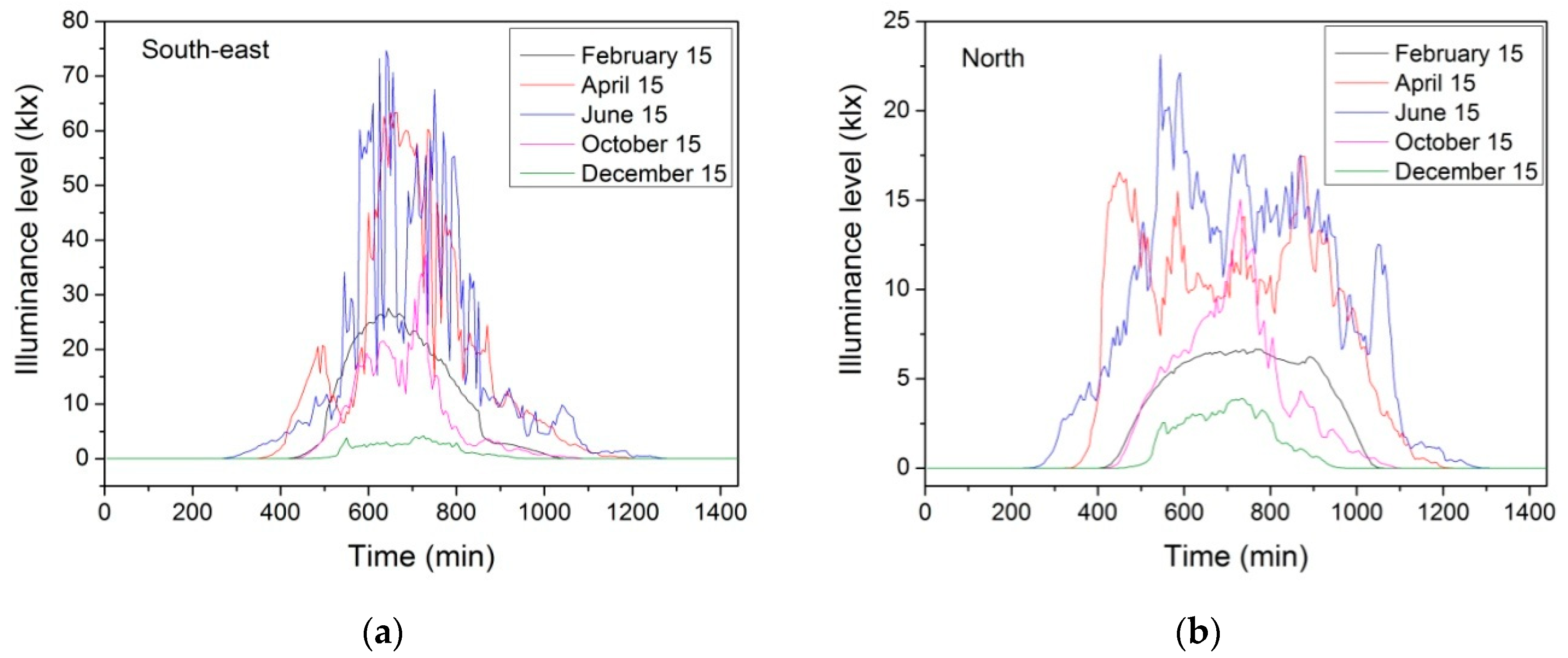
Obviously, daylight illuminance depends on the month and, in general, it is greatest in the summer months. Figure 7 shows the illuminance levels on the south-east and north façades measured every two months. The highest illuminance of approximately 72 klx was recorded on 15 June on the south-east façade. At the same time the maximum illuminance measured on the north façade reached 27 klx. The lowest maximum value of about 6 klx and the shortest time of its occurrence (about 7 h) was observed on 15 December. The illuminance measured on the north side was approximately 1.5 to 4 times lower than the illuminance measured on the south-east side of the building.
4.2. Availability of Daylight in the Classrooms Oriented to the North and South-East
The experimental investigations were carried out in the real classroom receiving daylight through windows located on one side of the wall of the room facing the south-east. To examine the impact of building orientation on daylight availability it was assumed that the identical room was located in such a way that the windows were north-facing.
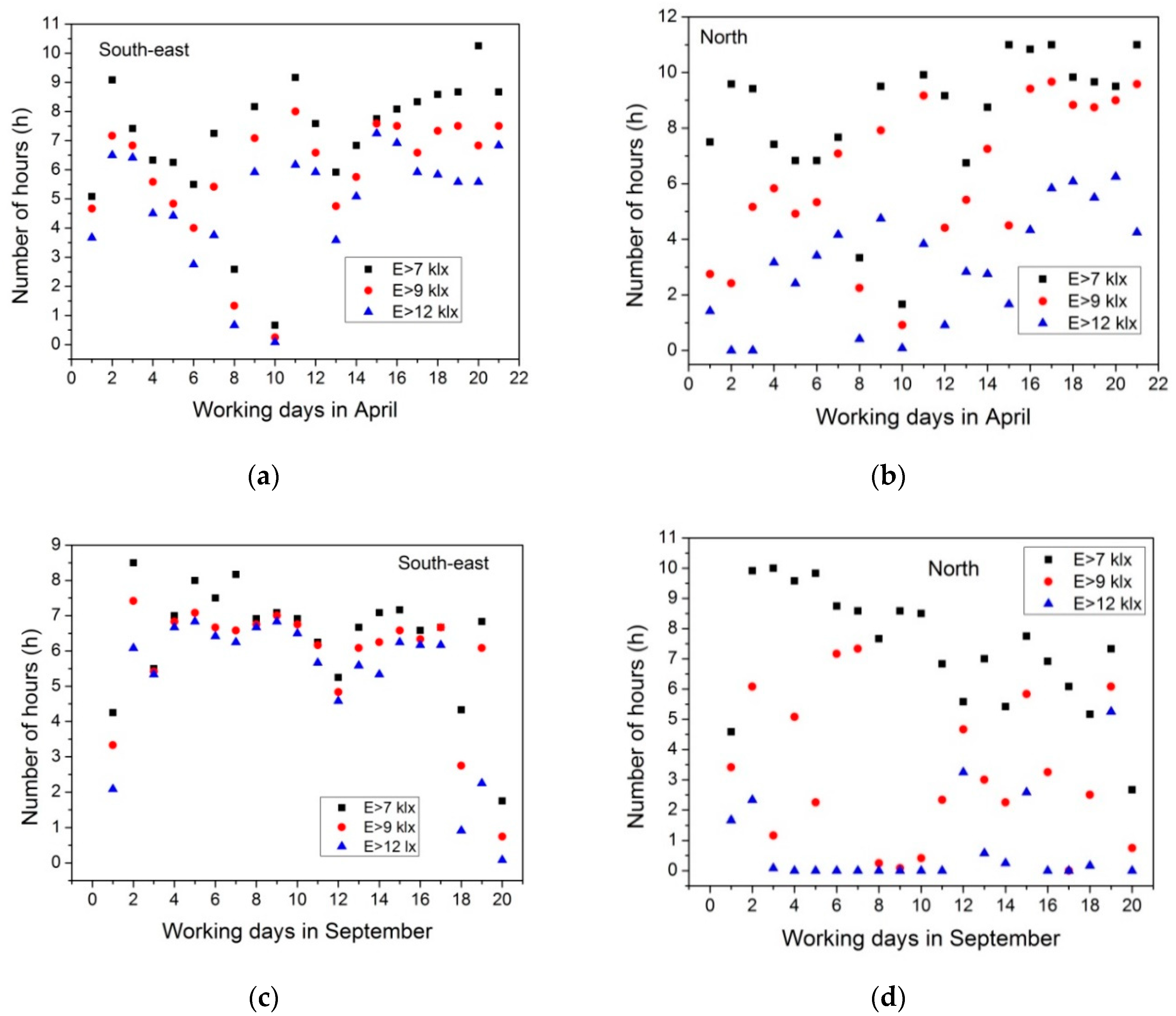
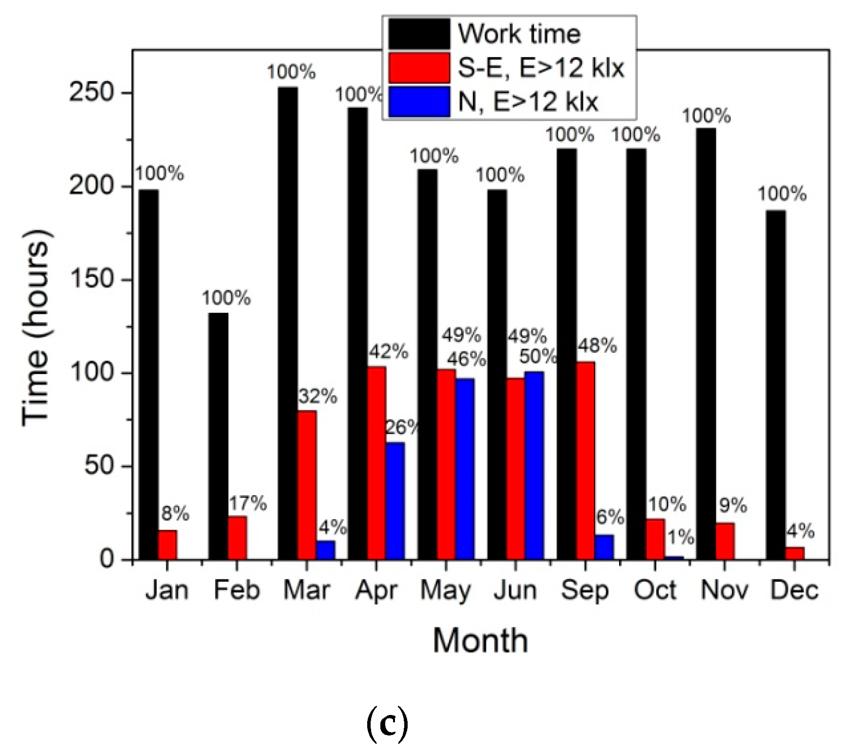
In order to assess the validity of lighting control and energy savings, the number of hours with illuminance levels higher than 7, 9, and 12 klx were estimated for one year, respectively, taking into account days of the university’s activity. These values were determined based on the recorded data from the SKNX and EIEE Laboratory and took into account the variation of the illuminance resulting from cloud cover. Figure 8 shows a comparison between the number of hours higher than the specified values from the south-east and north of the building for each day of the month. The results reveal a large variation in daylight availability in the rooms, especially in the month of April. In that month, more hours with illuminance level higher than 7 and 9 klx were from the north than south-east (Figure 8a,b). In September, it was similar only for illuminance level higher than 7 klx (Figure 8c,d). These relationships are also clearly visible in Figure 9. In April, the illuminance level on the south-east side exceeded 7 klx for 12 h less than on the north side; the number of hours with illuminance higher than 9 klx was almost the same on both sides; the illuminance exceeded 12 klx on the south-east side for about 40 h longer than on the north side. In September, on the south-east side, the illuminance level was higher than 7 klx for 18 h less than on the north side; the number of hours with the illuminance higher than 9 klx was bigger by half than on the north side, and the time when illuminance exceeds 12 klx is about 8 times longer on the south-east side than on the north. Considering all the months of university activity, it was observed that the number of hours on the north was higher than on the south-east side: with the illuminance level exceeding 7 klx—in the months from March to September, exceeding 9 klx—from April to June, and 12 klx—only in the month of June. Figure 9 also shows the work time specified taking into account that university lectures start at 7.30 a.m. and end at 6.30 p.m.; thus, the classroom occupancy time of classroom was 11 h.
4.3. Assessment of Lighting Energy Savings Potential
The results shown in Figure 8 and Figure 9 are of key importance for the assessment of an effective control strategy. On their basis, it can be predicted that because of the small number of hours in which the illuminance level was higher than 12 klx, the on/off control is much less energy efficient than dimming control. Furthermore, in a south-east-oriented classroom it was possible to turn off the lighting more often than in a north-facing one; hence, energy savings will be greater. Based on these results and the control strategy described in Section 3.2, the electricity consumption and energy savings potential are calculated. First, for on/off control, the annual number of hours of classroom activity when outdoor daylight was higher than 12 klx, was determined using the results shown in Figure 9c. The number of hours with daylight lower than 12 klx is the remainder of the classroom activity time. During that time, all lamps with a total power of 648 W were switched on and energy consumption was calculated as the product of the lighting time of the lamps and their power. Next, for dimming control, the number of hours when daylight was higher than 7 klx and lower than 9 klx (Figure 9a,b) was estimated, and during that time the lamps in the third row had to be turned on, those in the second row had to be brightened to 50%, and thus the power of 324 W was used. The time when daylight illuminance outside the building was higher than 9 klx and lower than 12 klx was determined based on Figure 9b,c, and then only the lamps in the third row had to be brightened to 50%, consuming the power of 108 W. When daylight illuminance outside the building was lower than 7 klx all the lamps were turned on, with a total power of 648 W. The time of that particular case was calculated as a difference between the number of hours during classroom activity and the number of hours shown in Figure 9a.
Energy savings potential is defined as the difference between electricity consumption without control (given in Section 3.1 and equal to 1354 kWh) and with control, referred to electricity consumption without control. The calculated electricity consumption per square meter of the classroom area and the energy savings potential are presented in Table 1.
The results show that the energy saving potential through the implementation of on/off control reached about 28% and this value is similar to the results obtained by Lo Verso and Pellegrino [17]. However, it should be noted that this value is obtainable for a classroom oriented to the south-east. For a north-oriented classroom the potential of energy savings is two times lower.
The use of dimming control allows a bigger reduction of electricity consumption, but also, which seems particularly important, the electricity saving potential for the location of the room on the north side of the building is only slightly smaller than for the room facing the south-east.
4.4. Economic Analysis of Lighting Control Strategies
Lighting control requires the implementation of a control system, which involves investment costs. Therefore, the question is about the relationship between investment costs and the reduction of energy bills and consequently the payback time of these investments. The analysis of this problem was carried out on the example of the educational building of the Poznan University of Technology. The building has five floors, each with identical nine classrooms oriented to the south-east. The total area of these classrooms is 2734 m2. For lighting control, a KNX standardized building automation system is proposed. The KNX device has a microcontroller, operating system, and memories (ROM, EEPROM, and RAM) and, being connected to the KNX bus communicates with other KNX devices using standard telegrams. On/off lighting control requires that the lamps in each room should be switched on by one channel of the switch actuator, so 45 channels are needed. For this purpose, it was proposed to use six Switch Actuators 8-fold. To measure the daylight illuminance level, a brightness sensor should be installed on the south-eastern elevation. All actuators and the sensor will be connected to one KNX bus line and supplied from Bus Power Supply of 640 mA. The actuators and bus power supply were produced by MDT technologies GmbH and the sensor was made by Theben company; device prices were taken from manufacturer catalogues. This system must be programmed using a PC with the installed Engineering Tool Software via a KNX/IP router. The costs of system installation and programming, often used in Polish practice, amounting to 15% of the equipment costs were assumed. The total cost of implementing the on/off lighting control system was estimated at PLN 16,206.
The dimming system is much more expensive because it requires that three rows of lamps in each room be switched on (or brightened) by one channel of the dimming actuator, so 135 channels are needed. It was proposed to use 35 Dimming Actuators 4-fold (seven to control the lamps on each floor) produced by MDT technologies GmbH and the same brightness sensor and bus power supply as for the on/off control. The total cost of implementing the on/off lighting control system including installation and programming costs was estimated at PLN 52,939.
Taking into account electricity consumption per square meter given in Table 1, and the total classroom area, the electricity consumption was calculated. The results are shown in Table 2. The table also presents the electricity costs, cost savings determined as a difference between electricity costs without and with lighting control, and payback time. In Poland, the unit cost of electricity is 0.67 PLN/kWh.
The greatest reduction in electricity costs is achieved by implementing the dimming control strategy. Payback time is about two years for both south-east and north orientation of the building. The time is shorter for the on/off control strategy due to significantly lower investment costs, but energy savings are a lot lower. It should be noted that the payback time depends on the cost of the system and devices, and their prices vary greatly by manufacturer. However, lighting control systems are becoming more frequent and cheaper while electricity prices are rising. In addition, the problem of reducing energy consumption and carbon dioxide emissions is becoming increasingly crucial.
5. Energy Saving Assessment Using the Method of Standard EN 15193-1
In Europe, lighting design in buildings must follow the EN 15193 1: 2017-08 standard, which allows the determination of the energy consumption for lighting per square meter of room area per year. In the last version of this standard, great importance was attached to the influence of daylight availability and daylight-depending lighting control on energy savings. To assess electricity consumption many arbitrary factors are used, including the geographical location of the building, its structure and dimensions, as well as lighting control methods. However, climatic conditions and building forms vary widely from one European country to another. Furthermore, recently, a wide variety of lighting control systems and strategies have been used. Considering the above, the estimation of energy consumption by other methods based on experimental research and comparison with consumption calculated according to the standard for a real building, its surroundings, and the selected lighting control strategy, is of great practical importance. The EN 15193 1: 2017-08 standard provides an estimation of electricity consumption for lighting in buildings by defining the LENI (lighting energy numeric indicator) expressed in kWh/(m2∙year). The LENI index takes into account the energy consumed by the luminaires; the energy consumed by the charging circuit of emergency lighting as well as the control system. In order to compare the electricity consumption estimated in Section 4.3 with the LENI index, further calculations take into account the first component only, i.e., the electricity consumed by the luminaires. This component is determined as
where: Pn is luminaires power in the room in W, Fc is constant illuminance factor; for calculation purposes, this factor is assumed to be 1.0, tD and tN are daylight time and non-daylight time usage respectively, in hours, FO is occupancy dependency factor, FD is daylight dependency factor, and A is floor area inside the outer walls in m2.
The daylight dependency factor FD is related to the daylight supply factor FD,S, and the lighting control factor FD,C. The first one takes into account the geometric boundary conditions expressed by the transparency index IT, the depth index IDe, and the obstruction index IO. In this case study the maximum possible depth of room covered by daylight is aD,max = 5.225 m, and the depth of classroom aD < 1.25·aD,max; thus, the real depth of the space can be used to calculate the area AD of horizontal working plane benefiting from natural lighting. The width of daylight zone AD corresponds to the dimension bD of the room façade. It means that the daylight zone coincides with the whole area of the classroom. Finally, the transparency index IT of the part of the building, which receives daylight, defined as IT = AC/AD amounts to 0.332. The depth index IDe = aD/(hLi − hTa) of the space covered by daylight is calculated using the geometrical parameters given in Section 3.1 and its value is 2.584. The obstruction index IO includes the shading of the building and is assumed to be 1.
The geometric indices IT, IDe and IO allowed to estimate the daylight factor DC = 7.256% for the carcass façade opening, which characterizes daylight availability to the zone. The value of this factor is reduced considering the impact of the fenestration and shading system on the daylight illumination levels by taking into account the direct hemispherical transmission of fenestration and three factors accounting for frame of fenestration system (typically 0.7), dirt on glazing (taken as 0.8), and not normal light incidence on façade (taken as 0.85). The direct hemispherical transmission of fenestration for windows in the considered classroom is 0.73.
The daylight factor D calculated using the assumed values is 2.521%. The impact of the fenestration and sun-protection system on daylight penetration can be judged by using Dc or D as indicated in Table 3 [18].
Calculations for the considered room show that with the use of the DC factor the daylight penetration will be strong, while taking into account the D factor the classroom will be classified as a medium-access room and this criterion was used to calculate the daylight supply factor FD,S. For the Poznan location at north latitude 52°, FD, S amount to 0.6341.
The second factor included in the calculation of daylight dependency factor FD is the lighting control factor FD,C describing the effectiveness of the artificial lighting control system. The EN 15193 1: 2017-08 standard gives the correction factor FD,C for daylight delivery depending on the room classification in terms of daylight availability and type of lighting control. For a room with medium light access and automatic control, FD,C amounts to 0.77. Taking into account the obtained values of the FD,S and FD,C, the factor depending on daylight FD equals 0.512.
Occupancy dependency factor FO depends on the proportion FA of the time that the space is unoccupied which should be 0.25 in accordance with the standard for classrooms in educational buildings. Taking into account on/off lighting control and the fulfillment of a condition 0.2 ≤ FA ≤ 0.9, the occupancy dependency factor is 0.85.
In LENI calculation, the operating hours during the daylight time tD is taken as experimentally recorded time when the daylight illuminance level was higher than 12 klx and non-daylight time tN as the difference between the total university activity time of the year and daylight time tD. The calculation results are presented in Table 4.
The comparison of electricity consumed for lighting given in Table 1 and the LENI from Table 4 shows that these values are almost identical for the classroom oriented to the south-east and only slightly different for that oriented to the north. This applies to on/off lighting control. This good agreement of the experiment and calculation results from an accurate determination of daylight availability in the classroom. Nevertheless, it should be noted that in the LENI calculation, the daylight supply factor FD,S is determined using approximated relation as a function of site latitude and does not take into account room orientation. The difference in LENI values for the south-east and north orientation is only the result of daylight time availability.
It is worth noting that a similar comparison for dimming control is not possible due to the differences in the control strategies considered in this work and in the EN 15193 1: 2017-08 standard. As regards the standard, the dimming strategy takes into account daylight penetration (weak, medium, and strong), automatic presence or absence detection, and the proportion of the time when the space is unoccupied. The values of specific factors are given for different conditions. It is also assumed that the dimming of the luminaires to a certain illuminance level occurs throughout the room. A dimming strategy that takes into account the distribution of daylight illuminance in room depth is not considered.
6. Conclusions
In this paper, the influence of building orientation on daylight availability in a typical educational building in Poland was investigated. Measurements of daylight illuminance distributions in the room depth allowed us to determine that, with daylight illuminance outside the building greater than 12 klx, the required illuminance of 0.5 klx is reached in the whole working plane, and luminaires in the classroom could be turned off. For the illuminance level lower than 7 klx, all luminaires should be turned on. In addition, two outdoor daylight illuminance ranges were defined, namely between 7 and 9 klx and between 9 and 12 klx, for which some luminaires in the classroom could be turned off and some could be dimmed. Using the daylight illuminance recorded in the SKNX and EIEE Laboratory at the Poznan University of Technology, the number of hours per year of the university’s activity during which the lighting had to be switched on (up to 100% or brightened) was determined. This illuminance was measured on the south-eastern façade of the building by a weather station and on the north façade by an additional brightness sensor and recorded using KNX BACS field network implemented in the building. Based on that number of hours, it was predicted that due to the small amount of time when the illuminance level was higher than 12 klx, the on/off control was much less energy efficient than dimming control. Furthermore, in a south-east-oriented classroom, it is possible to turn off the lighting more often than in a north-oriented one; hence, the energy savings will be larger. This finding is well seen in the calculated electricity consumption and potential of energy savings for two lighting control strategies. For a classroom facing the south-east, the energy saving potential through the implementation of the on/off control reached about 28% of electricity consumed without control. For a north-oriented classroom the potential of energy savings was two times lower. The use of dimming control allows a bigger reduction of electricity consumption, but also, which seems particularly important, the energy saving potential for the location of the room on the north side is only slightly smaller than for the room on the south-east side. This proves that by using dimming control depending on daylight distribution in a room; comparable energy savings can be achieved for different building orientations. It is worth noting that the obtained results can be generalized to office and public buildings, where, according to the building standard, the ratio of window area calculated in the frame opening to floor area must, as mentioned above, be at least 1:8. In such buildings, daylight availability and daylight distribution in the room depth are similar.
For the implementation of the described on/off and dimming control strategies, KNX building automation systems were proposed and their investment costs were estimated. These costs were compared with the reduction in energy bills due to energy savings for lighting, and payback times were calculated. In the case of dimming control, payback time can be about two years, while it is shorter for on/off control due to significantly lower investment costs.
The electricity consumption estimated experimentally was compared with the LENI calculated according the standard EN 15193 1: 2017. Particular attention was paid to the accuracy of the LENI estimation and the possibility of obtaining the value of this indicator in the real building. The comparison shows that these values are almost identical for the classroom oriented to the south-east and only slightly different for that oriented to the north. This applies to on/off lighting control, while a similar comparison for dimming control is not possible due to the differences in the control strategies considered in this work and in the EN 15193 1: 2017-08 standard. This good agreement of the experiment and calculation results from an accurate determination of daylight availability in the classroom. Nevertheless, it should be noted that in the LENI calculation, the daylight supply factor FD,S is determined using approximated relation as a function of site latitude and does not take into account room orientation. The difference in LENI values for south-east and north orientation is only the result of daylight time availability.
Estimation of electricity consumption and energy savings was carried out taking into account the requirements given in the standard EN 12464-1 “Lighting of workplaces—Indoor work places”. Three lighting design classes are proposed as quality ones: basic fulfillment of requirements, good fulfillment of requirements, and comprehensive fulfillment of requirements. The power of luminaires per square meter of educational room area assigned to these classes are respectively: 15, 20, and 25 W/m2. The results shown in Table 1 and the LENI were calculated assuming 20 W/m2 as the power per square meter of room area; thus, the value corresponds to a quality educational classroom specified as “good fulfillment of requirements”. In lighting design, DIALux or RELUX software is used and various types of luminaires are selected from manufacturers’ catalogues. Relating the lamp power to a square meter of room area allows easy calculation of electricity consumption with the use of a different lamp power, since electricity consumption is proportional to the power of the lamps per square meter of room area.
Funding
This research received no external funding.
Acknowledgments
This study is based upon work supported by the National Centre for Research and Development in the context of the Innovative Economy Program under grant No. POIG.02.02.00-00-018/08. This work was also supported by the 2018 Poznan University of Technology funds transferred from the Ministry of Science and Higher Education.
Conflicts of Interest
The author declares no conflict of interest. The funders had no role in the design of the study; in the collection, analyses, or interpretation of data; in the writing of the manuscript, and in the decision to publish the results.
References
- Dilaura, D.L.; Houser, K.W.; Mistrick, R.G.; Steffy, G.R. The Lighting Handbook, 10th ed.; The Illuminating Engineering Society of North America: New York, NY, USA, 2011. [Google Scholar]
- Wang, J.; Wei, M.; Chen, L. Does typical weather data allow accurate predictions of daylight quality and daylight-responsive control system performance. Energy Build. 2019, 184, 72–87. [Google Scholar] [CrossRef]
- Eriksson, S.; Waldenström, L.; Tillberg, M.; Österbring, M.; Kalagasidis, A.S. Numerical Simulations and Empirical Data for the Evaluation of Daylight Factors in Existing Buildings in Sweden. Energies 2019, 12, 2200. [Google Scholar] [CrossRef] [Green Version]
- Mardaljevic, J. Climate-based daylight modelling and its discontents. In Proceedings of the CIBSE Technical Symposium, London, UK, 16–17 April 2015. [Google Scholar]
- Nabil, A.; Mardaljevic, J. Useful daylight illuminance: A new paradigm to access daylight in buildings. Lighting Res. Technol. 2005, 37, 41–59. [Google Scholar] [CrossRef]
- Reinhart, C.F.; Mardaljevic, J.; Rogers, Z. Dynamic daylight performance metrics for sustainable building design. Leukos 2006, 3, 7–31. [Google Scholar] [CrossRef] [Green Version]
- Nabil, A.; Mardaljevic, J. Useful daylight illuminances: A replacement for daylight factors. Energy Build. 2006, 38, 905–913. [Google Scholar] [CrossRef]
- Reinhart, C.F.; Weissman, D.A. The daylit area—Correlating architectural student assessments with current and emerging daylight availability metrics. Build. Environ. 2012, 50, 155–164. [Google Scholar] [CrossRef]
- Mangkuto, R.A.; Fathurrahman, F.; Eka Putra, R.; Atmodipoero, R.T.; Favero, F. Optimisation of daylight admission based on modifications of light shelf design parameters. J. Build. Eng. 2018, 18, 195–209. [Google Scholar] [CrossRef]
- Mangkuto, R.A.; Rohmah, M.; Asri, A.D. Design optimisation for window size, orientation, and wall reflectance with regard to various daylight metrics and lighting energy demand: A case study of buildings in the tropics. Appl. Energy 2016, 164, 211–219. [Google Scholar] [CrossRef]
- Gioia, F. Search for the optimal window-to-wall ratio in office buildings in different European climates and the implications on total energy saving potential. Solar Energy 2016, 132, 467–492. [Google Scholar] [CrossRef]
- Troup, L.; Phillips, R.; Eckelman, M.J.; Fannon, D. Effect of window-to-wall ratio on measured energy consumption in US office buildings. Energy Build. 2019, 203. [Google Scholar] [CrossRef]
- IEA (International Energy Agency). Guidebook on Energy Efficient Electric Lighting for Buildings; ANNEX 45 Report. ECBCS—Energy Conservation in Buildings and Community, Systems; Halonen, L., Tetri, E., Bhusal, P., Eds.; AECOM Ltd.: St Albans, UK, 2010. [Google Scholar]
- Rubeis, T.; Nardi, I.; Muttillo, M.; Ranieri, S.; Ambrosini, D. Room and window geometry influence for daylight harvesting maximization—Effects on energy savings in an academic classroom. Energy Procedia 2018, 148, 1090–1097. [Google Scholar] [CrossRef]
- Li, D.H.W.; Cheung, A.C.K.; Chow, S.K.H.; Lee, E.W.M. Study of daylight data and lighting energy savings for atrium corridors with lighting dimming controls. Energy Build. 2014, 72, 457–464. [Google Scholar] [CrossRef]
- Haq, M.A.; Hassan, M.Y.; Abdullah, H.; Rahman, H.A.; Abdullah, M.P.; Hussin, F.; Said, D.M. A review on lighting control technologies in commercial buildings, their performance and affecting factors. Renew. Sustain. Energy Rev. 2014, 33, 268–279. [Google Scholar] [CrossRef]
- Lo Verso, V.R.M.; Pellegrino, A. Energy Saving Generated Through Automatic Lighting Control Systems According to the Estimation Method of the Standard EN 15193-1. J. Daylighting 2019, 6, 131–147. [Google Scholar] [CrossRef] [Green Version]
- European Committee for Standardization. EN 15193-1:2017. Energy Performance of Buildings—Energy Requirements for Lighting; European Committee for Standardization (CEN): Brussels, Belgium, 2017. [Google Scholar]
- Rubeis, T.; Muttillo, M.; Pantoli, L.; Nardi, I.; Leone, I.; Stornelli, V.; Dario, A. A first approach to universal daylight and occupancy control system for any lamps: Simulated case in an academic classroom. Energy Build. 2017, 152, 24–39. [Google Scholar] [CrossRef] [Green Version]
- Kaminska, A.; Ożadowicz, A. Lighting Control Including Daylight and Energy Efficiency Improvements Analysis. Energies 2018, 11, 2166. [Google Scholar] [CrossRef] [Green Version]
- European Committee for Standardization. EN 12464 Light and Lighting—Lighting of Work Places—Part 1: Indoor Work Places; European Committee for Standardization (CEN): Brussels, Belgium, 2012. [Google Scholar]
- Li, D.H.W. A review of daylight illuminance determinations and energy implications. Appl. Energy 2010, 87, 2109–2118. [Google Scholar] [CrossRef]
Figure 1.
External view of the SKNX and EIEE Laboratory building (1) and the educational building of the Poznan University of Technology (2), from https://www.google.com/maps on 20.10.2019.
Figure 1.
External view of the SKNX and EIEE Laboratory building (1) and the educational building of the Poznan University of Technology (2), from https://www.google.com/maps on 20.10.2019.

Figure 2.
Layout of the laboratory with the arrangement of lamps and measuring grid.

Figure 3.
Daylight illuminance level distributions in the classroom depth in April and illuminance level outside the building of 8600 lx.
Figure 3.
Daylight illuminance level distributions in the classroom depth in April and illuminance level outside the building of 8600 lx.

Figure 4.
Various waveforms of daylight illuminance level measured by the weather station.

Figure 5.
Illuminance levels of daylight measured at the same time by the sensors located on the south-east (S-E) and north (N) side of the building.
Figure 5.
Illuminance levels of daylight measured at the same time by the sensors located on the south-east (S-E) and north (N) side of the building.

Figure 6.
Illuminance levels of daylight measured by sensors located on the south-east (S-E) and north (N) side of the building in winter on an overcast day (a) and on a sunny day (b), as well as in the summer, on a sunny day (c).
Figure 6.
Illuminance levels of daylight measured by sensors located on the south-east (S-E) and north (N) side of the building in winter on an overcast day (a) and on a sunny day (b), as well as in the summer, on a sunny day (c).

Figure 7.
Illuminance levels of daylight measured by sensors located on the south-east (a) and north (b) side of the building, recorded every two months.
Figure 7.
Illuminance levels of daylight measured by sensors located on the south-east (a) and north (b) side of the building, recorded every two months.

Figure 8.
Number of hours in which the illuminance level outside the building exceeded the value of 7, 9, and 12 klx, on working days in April, from the south-east (a) and the north (b), and in September, from the south-east (c) and the north (d).
Figure 8.
Number of hours in which the illuminance level outside the building exceeded the value of 7, 9, and 12 klx, on working days in April, from the south-east (a) and the north (b), and in September, from the south-east (c) and the north (d).

Figure 9.
Number of hours during the university’s activity when the illuminance level outside the building exceeded the value of 7 (a), 9 (b), and 12 klx (c) from the south-east (S-E) and the north (N).
Figure 9.
Number of hours during the university’s activity when the illuminance level outside the building exceeded the value of 7 (a), 9 (b), and 12 klx (c) from the south-east (S-E) and the north (N).


Table 1.
Electricity consumption and energy savings potential.
| LIGHTING CONTROL | Electricity Consumption (kWh/m2) | Energy Savings Potential (%) | ||
|---|---|---|---|---|
| South-East | North | South-East | North | |
| Without control | 43.24 | 43.24 | 0 | 0 |
| On/off control | 31.35 | 37.34 | 27.50 | 13.64 |
| Dimming control | 27.93 | 29.63 | 35.42 | 31.48 |
Table 2.
Electricity consumption and costs as well as cost savings and payback time.
| LIGHTING CONTROL | Electricity Consumption kWh | Electricity Costs PLN | Cost Savings PLN | Payback Time Years | ||||
|---|---|---|---|---|---|---|---|---|
| South-East | North | South-East | North | South-East | North | South-East | North | |
| Without control | 118,218 | 118,218 | 79,206 | 79,206 | 0 | 0 | 0 | 0 |
| On/off control | 85,711 | 102,088 | 57,426 | 68,399 | 21,780 | 10,808 | 0.74 | 1.5 |
| Dimming control | 76,307 | 81,008 | 51,162 | 54,276 | 28,045 | 24,931 | 1.9 | 2.1 |
Table 3.
Daylight penetration as function of the daylight factor DC for the carcass façade opening and daylight factor D for the zone, according to EN 15193 1: 2017-08 [18].
Table 3.
Daylight penetration as function of the daylight factor DC for the carcass façade opening and daylight factor D for the zone, according to EN 15193 1: 2017-08 [18].
| Classification | Daylight Penetration | |
|---|---|---|
| DC | D | |
| Dc ≥ 6% | D ≥ 3% | Strong |
| 6% > Dc ≥4% | 3% > D ≥ 2% | Medium |
| 4% > Dc ≥ 2% | 2% > D ≥ 1% | Weak |
| Dc < 2% | 1 < D% | None |
Table 4.
LENI calculated according to EN 15193 1: 2017-08 and potential of energy savings.
| Classroom Orientation | LENI (kWh/(m2·Year)) | Potential of Energy Saving (%) |
|---|---|---|
| Without control | 43.24 | 0 |
| South-east, on/off control | 31.82 | 26.41 |
| North, on/off control | 34.31 | 20.65 |
© 2020 by the author. Licensee MDPI, Basel, Switzerland. This article is an open access article distributed under the terms and conditions of the Creative Commons Attribution (CC BY) license (http://creativecommons.org/licenses/by/4.0/).
Share and Cite
MDPI and ACS Style
Kaminska, A. Impact of Building Orientation on Daylight Availability and Energy Savings Potential in an Academic Classroom. Energies 2020, 13, 4916. https://0-doi-org.brum.beds.ac.uk/10.3390/en13184916
AMA Style
Kaminska A. Impact of Building Orientation on Daylight Availability and Energy Savings Potential in an Academic Classroom. Energies. 2020; 13(18):4916. https://0-doi-org.brum.beds.ac.uk/10.3390/en13184916
Chicago/Turabian StyleKaminska, Aniela. 2020. "Impact of Building Orientation on Daylight Availability and Energy Savings Potential in an Academic Classroom" Energies 13, no. 18: 4916. https://0-doi-org.brum.beds.ac.uk/10.3390/en13184916
Note that from the first issue of 2016, this journal uses article numbers instead of page numbers. See further details here.