Parameter Calibration for a TRNSYS BIPV Model Using In Situ Test Data

Abstract

Installing renewable energy systems for zero-energy buildings has become increasingly common; building integrated photovoltaic (BIPV) systems, which integrate PV modules into the building envelope, are being widely selected as renewable systems. In particular, owing to the rapid growth of information and communication technology, the requirement for appropriate operation and control of energy systems has become an important issue. To meet these requirements, a computational model is essential; however, some unmeasurable parameters can result in inaccurate results. This work proposes a calibration method for unknown parameters of a well-known BIPV model based on in situ test data measured over eight days; this parameter calibration was conducted via an optimization algorithm. The unknown parameters were set such that the results obtained from the BIPV simulation model are similar to the in situ measurement data. Results of the calibrated model indicated a root mean square error (RMSE) of 3.39 °C and 0.26 kW in the BIPV cell temperature and total power production, respectively, whereas the noncalibrated model, which used typical default values for unknown parameters, showed an RMSE of 6.92 °C and 0.44 kW for the same outputs. This calibration performance was quantified using measuring data from the first four days; the error increased slightly when data from the remaining four days were compared for the model tests.

1. Introduction

In many developed countries, the sector that accounts for the greatest percentage of energy use is building construction [1,2]. A general approach to mitigating energy consumption in this sector is improving thermal insulation, which is effective in reducing HVAC energy consumption. Energy production from renewable energy systems is mandatory in several countries to ensure the sector is zero-energy [3] or positive-energy for the future. Recently, various renewable energy systems have been installed to supply a large portion of the required energy in buildings via on-site energy production.

The building integrated photovoltaic (BIPV) system is one of the most popular renewable energy systems for achieving zero-energy buildings. The photovoltaic (PV) cell array of the BIPV module is enclosed in transparent building material, such as window glass or double-skin facades, and it converts building envelopes to a power generation system. These BIPV modules can be installed on any of the building skins, while the installation of a typical PV module is limited to rooftops or surplus areas besides the building. Thus, the BIPV system is effective, particularly for buildings with a curtain wall.

The BIPV system generates electricity via a simple mechanism, with high durability and without any specific problems. Therefore, the BIPV system is regarded as a promising and practical renewable energy system [4,5]. Consequently, the market share of the BIPV system has continuously increased, along with related studies [5,6].

The efficiency of BIPV can be categorized according to types of installation such as angle, direction, location, etc. [7]. Annual power generation per a typical BIPV module in Seoul for 2013 was 659.6 kWh/kWp·year when installed on vertical southwest wall and 626.6 kW/kWp·year on a horizontal roof [8].

An important and well-known issue concerning the performance of the BIPV system is that the PV cell temperatures inevitably increase during the process of generating electricity from solar energy [9]. The BIPV modules are scarcely cooled as they are installed on the building envelope; thus, the increased cell temperature decreases the overall efficiency of the BIPV system [9,10,11,12].

Despite such issues, several studies have focused on using the BIPV system more efficiently.

Table 1. Brief review of research on the BIPV system.

Authors	Year	Purpose of Studies	Methodologies
			Exp.	Simulation
S. Yadav & S.K. Panda [13]	2020	Finding the optimum angle	x	Mathematical model
J.E. Goncalves et al. [14]	2020	Predicting power generation	x	Mathematical model
R.A. Agathokleous et al. [17]	2018	Modeling and validation	x	Commercial software
M. Debbarma et al. [18]	2017	Modeling	-	Mathematical model
O. Hachana et al. [19]	2016	Fault detection & diagnosis	x	Mathematical model
W. Chine et al. [15]	2016	Fault detection & diagnosis	x	Data-driven model
S. Li et al. [16]	2015	Predictive control	x	Commercial software
E. Vuong et al. [20]	2015	Model development	-	Commercial software
L. Aelenei et al. [6]	2014	Model validation	x	Mathematical model
T. Yang & A.K. Athienitis [21]	2014	Model validation	x	Mathematical model
C.Y. Huang et al. [22]	2011	Model validation	x	Mathematical model
L. Liao et al. [23]	2007	Heat distribution prediction	-	CFD

presents details of some previous studies. These studies designed the capacity of the BIPV system by accounting for the rising cell temperature [13], predicting the amount of electrical power generation required to control the energy management system (EMS) [14], or implementing data-driven or mathematical models for fault detection and diagnosis (FDD) [15,16]. To conduct such studies, a simulation model that can describe and predict physical behaviors is essential.

As shown in Table 1, most studies were conducted by using simulations with self-developed or existing models, provided in commercial programs. However, the development of a mathematical model requires elaboration and time, particularly for debugging. Conversely, utilizing an existing model is useful and efficient as it requires less time; however, a limitation is that the system complexity and some physical relations among the system components relating to target cases are not fully reflected in the model. In addition, uncertainties in material properties, manufacturing, and installation quality are sporadic. Therefore, calibration of the simulation model may be required to describe the target case.

A comparison between model results and in situ test data is typically employed for model calibration. A common method to use existing models is parameter fitting using empirical data collected over a short period. The fitted model can then be used for long-term performance evaluation, such as BIPV electricity yield or various engineering works. Model-based FDD is one such example.

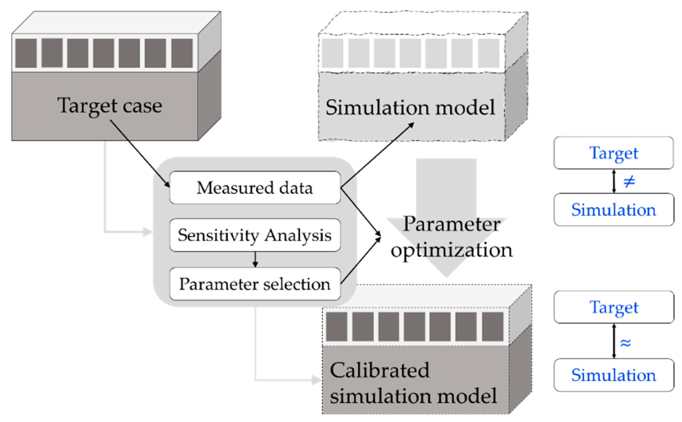
Figure 1 shows how an existing model can be used to depict a real target case in this work. An in situ test was performed for short period and a TRNSYS BIPV model was selected as the existing model. Then, the calibration is performed not only for the most sensitive parameters among unknown ones but also for physically uncertain parameters as a target case is not fully reflected in a model as mentioned earlier. The deviation between simulation and field tests was minimized through TRNOPT, which is parameter optimization tool implemented in TRNSYS. This paper presents a detailed process of this proposed methodology.

2. Materials and Methods

2.1. In Situ Measurement of the Target BIPV System

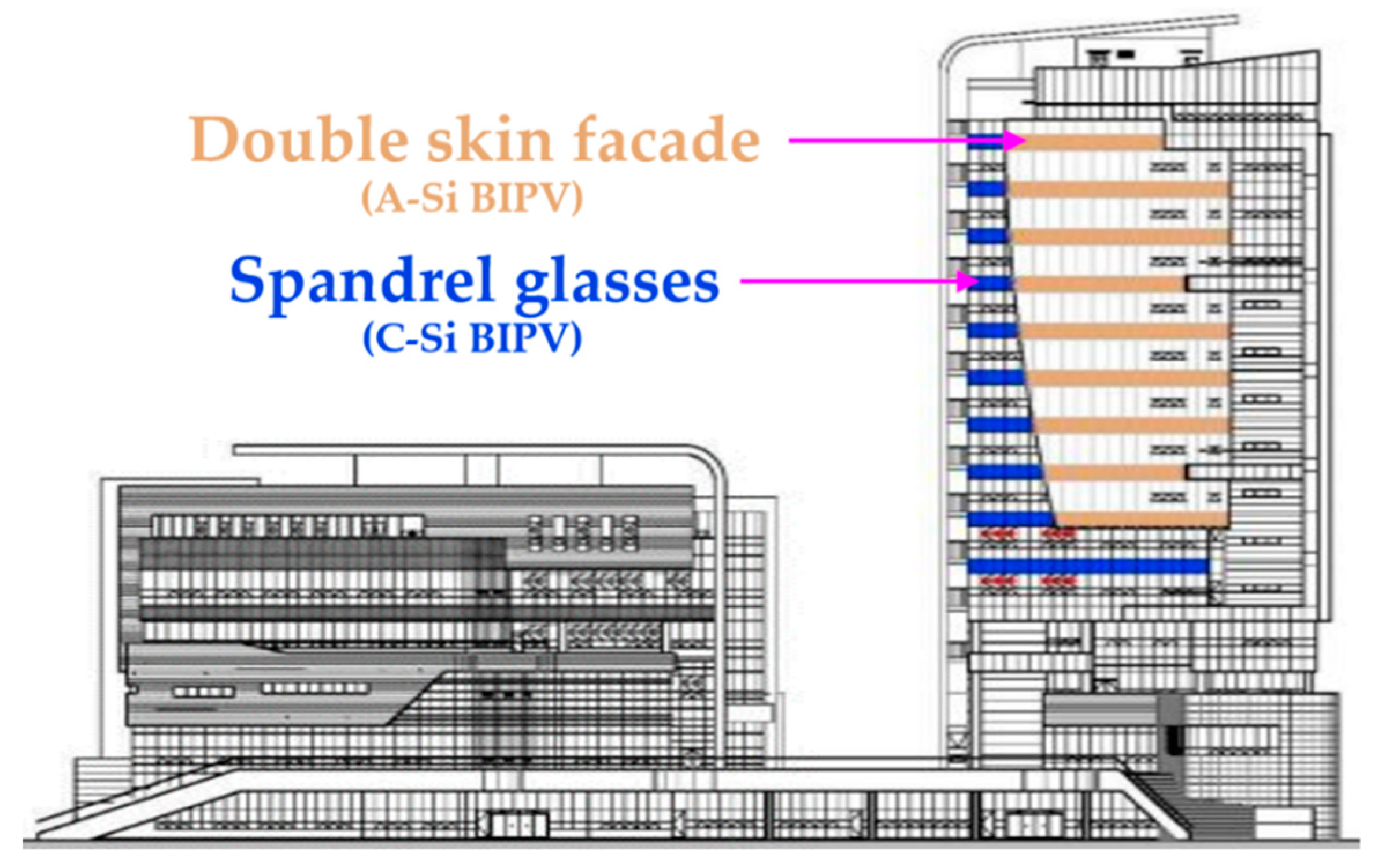
Figure 2 depicts the target test building, located in Incheon, South Korea. The country has a mild climate. For instance, in 2019, the highest temperature in Incheon was around 36 °C in summer, and about the lowest one was around −10.4 °C in winter. Total annual amount of solar irradiance was 1466.66 kWh/m² in Incheon, and this level is similar over the country.

A total of 58 polycrystalline Si (C-Si) BIPV modules were installed on the southern façade spandrel and 120 amorphous-Si (A-Si) BIPV modules were installed on the double-skin façade. The target system of this study consists of C-Si BIPV modules on the spandrel adjacent to the indoor ceiling space. Two arrays of 29 C-Si parallel-connected BIPV modules were investigated; the rated power of each BIPV module was 116 W, and the maximum power point voltage, V_MPP, and current, I_MPP, were 14.2 V and 8.17 A, respectively, under the standard temperature condition (STC, solar irradiance = 1000 W/m², air mass = 1.5 G, and cell temperature = 25 °C). The size of each module was 1.034 m², and the thickness of the back insulation material was 75 mm.

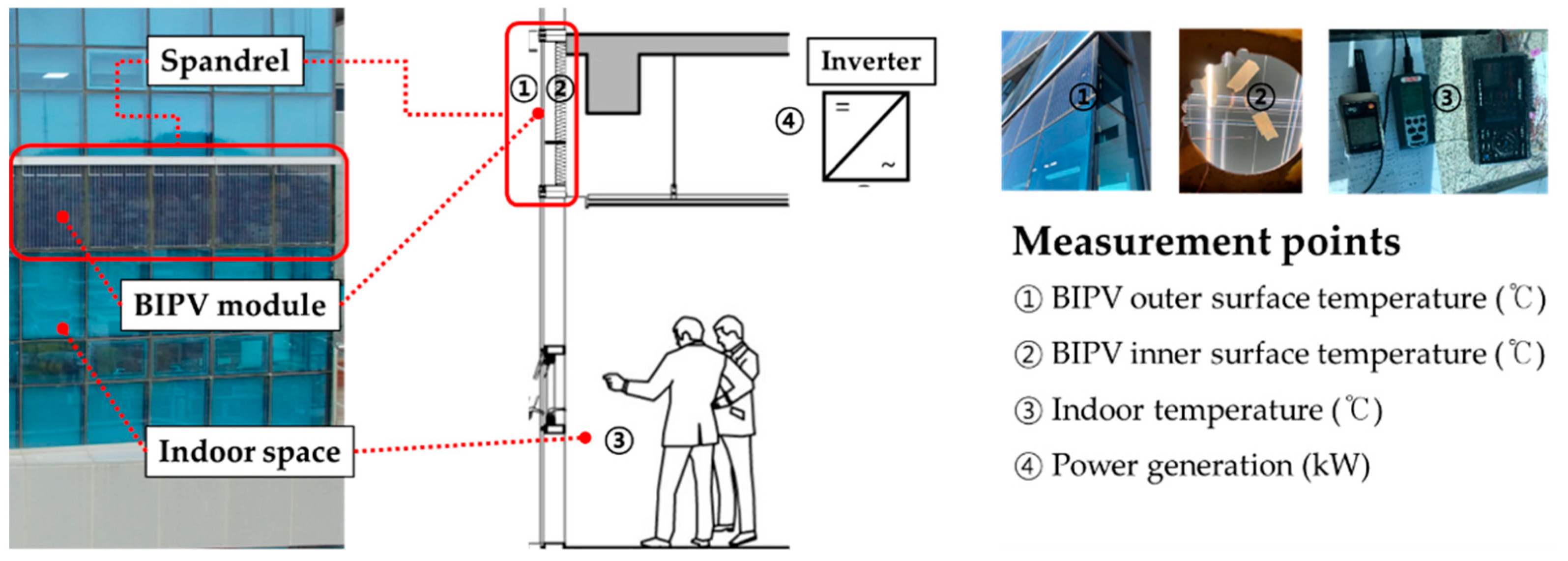
The BIPV module of the target building was fabricated from top to bottom, with the following order: outer cover glass, PV cells, substrate glass, air channel, and back insulation. The temperatures of the outer cover, substrate glass surface, and channel of the BIPV module were measured using thermocouples, and the indoor space temperature was measured using a Testo device. The power generated from the 58 BIPV modules was also measured via a DC meter from the inverter inlet. Daily meteorological data, including total horizontal solar radiation and temperatures, were obtained from the website of the Korea Meteorological Administration (KMA), and the target total radiation along the southern orientation was calculated using a direct diffuse split model [24,25]. This selection of using meteorological data was made to ensure our fitted model is useful in the future, requiring only data from the KMA. The temperatures were measured for eight days, from 27 November to 4 December. Figure 3 presents details of the measurement location for the target BIPV system. Although the measuring instruments were installed in one module, the cell temperature of the BIPV module was assumed to be the average of the inner and outer surface temperatures of the module.

2.2. Theoretical Review of the TRNSYS BIPV Model

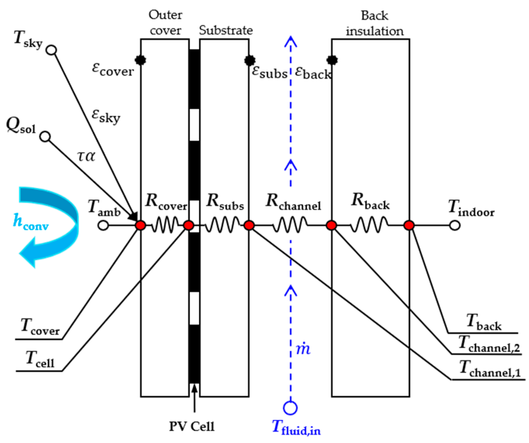
TRNSYS is a well-known dynamic energy simulation tool developed by Klein et al. [26], and the steady-state BIPV simulation model, type 567, is included in the model library. This model uses a thermal network of BIPV components, as shown in Figure 4.

The model can describe airflow within the air channel between the BIPV module and back insulation, with inlet airflow temperature and flow rate. The gray-colored calculation nodes represent the material layers for the BIPV cover, PV cells, substrate, and the front and back of the back insulation material of the BIPV module. The model inputs are indicated by the white nodes as boundary conditions, as follows: sky temperature, T_sky, ambient air temperature, T_amb, indoor temperature, T_indoor, and inlet air temperature of the channel, T_fluid,in. The resistances are set as model parameters, and they explain the thermal relations between nodes, together with the outdoor convection heat transfer coefficient, h_conv. The resistances can be deduced from the material properties, such as conductivity, emissivity, and thickness, or calibrated values, which will be discussed later.

Based on the thermal network in Figure 4, TRNSYS type 567 calculates the PV efficiency and power production using Equations (1)–(3). Here, ${\eta }_{\mathrm{BIPV}}$ is the BIPV module efficiency, ${\eta }_0$ is the reference PV efficiency at STC, ${\mathrm{EM}}_{\mathrm{R}}$ and ${\mathrm{EM}}_{\mathrm{T}}$ are the efficiency modifiers of the solar radiation and temperature, respectively, $Q_{\mathrm{ref}}$ and $T_{\mathrm{ref}}$ are the solar radiation and temperature of the STC, respectively, $Q_{\mathrm{sol}}$ is the solar irradiation, and $T_{\mathrm{cell}}$ is the calculated cell temperature:

$${\eta }_{\mathrm{BIPV}}={\eta }_0\times \left\{1+{\mathrm{EM}}_{\mathrm{R}}\times \left(Q_{\mathrm{sol}}-Q_{\mathrm{ref}}\right)\right\}\times \left\{1+{\mathrm{EM}}_{\mathrm{T}}\times \left(T_{\mathrm{cell}}-T_{\mathrm{ref}}\right)\right\},$$

(1)

$$\mathrm{IAM}=\frac{\tau \alpha }{\tau {\alpha }_{\mathrm{n}}}=1-0.1\times \left(\frac{1}{\cos \theta }-1\right),$$

(2)

$${\dot{E}}_{\mathrm{BIPV}}=\tau {\alpha }_{\mathrm{n}}\times \mathrm{IAM}\times {\eta }_{\mathrm{BIPV}}\times A\times Q_{\mathrm{sol}},$$

(3)

Type 567 uses the solar incident angle modifier proposed by ASHRAE [27]. The incident angle modifier (IAM) is defined by $\tau \alpha$ (product of transmittance and absorptance of the module under a given incident angle,$\theta$) or as $\tau {\alpha }_{\mathrm{n}}$ (the normal $\tau \alpha$) when $\theta$ is zero. The IAM is used to calculate the BIPV power production, ${\dot{E}}_{\mathrm{BIPV}}$, as shown in Equation (3). Here, A is the surface area of the BIPV module. Details of the parameters for the target BIPV modules are presented in

Table 2. Parameters of the target BIPV module.

Parameter	Value	Unit
Cover area ($A$)	1.034	m2
Cover thickness	0.005	m
Channel height	0.085	m
Cover thermal conductivity (1/$R_{\mathrm{cover}}$)	0.96	W/m·K
Substrate thermal resistance ($R_{\mathrm{subs}}$)	7.052	m·K/W
Back insulation thermal resistance ($R_{\mathrm{back}}$)	1.876	m·K/W
Normal transmittance-absorptance ($\tau {\alpha }_{\mathrm{n}}$)	0.85	-
Cover emissivity (${\epsilon }_{\mathrm{cover}}$)	0.9	-
Substrate emissivity (${\epsilon }_{\mathrm{subs}}$)	0.9	-
Back insulation emissivity (${\epsilon }_{\mathrm{back}}$)	0.9	-
Reference BIPV efficiency (${\eta }_{\mathrm{BIPV}}$)	14.1	%
Rated power (${\dot{E}}_{\mathrm{PV}}$)	116	W
Maximum power point voltage ($V_{\mathrm{MPP}}$)	14.2	V
Open circuit voltage	18.9	V
Maximum power point current ($I_{\mathrm{MPP}}$)	8.17	A
Short circuit current	8.71	A
Efficiency modifier—temperature (EMT)	−0.00039	°C−1
Efficiency modifier—solar radiation (EMR)	0.00009	m·K/W

.

$h_{\mathrm{conv}}$ can be simply calculated using the outdoor air velocity, $v$, as shown in Equation (4), the values for which are obtained from weather data. The sky temperature, $T_{\mathrm{sky}}$, can be represented by Equation (5) as a the function of ambient air temperature, $T_{\mathrm{amb}}$, sky emissivity, ${\epsilon }_{\mathrm{sky}}$, and cloud factor, $CF$, which has a range of 0–1 (for a clear sky, $CF$= 0) [28].

$$h_{\mathrm{conv}}=\frac{5.7+3.8v}{3.6},$$

(4)

$$T_{\mathrm{sky}}=T_{\mathrm{amb}}\times {\epsilon }_{\mathrm{sky}}+0.8\times {\left(1-{\epsilon }_{\mathrm{sky}}\times CF\right)}^{0.25},$$

(5)

The values of all the presented parameters are given in Table 2; these were obtained from the manufacturer’s documentation of the BIPV module and meteorological data. However, parameters such as surface emissivity, transmittance, absorptance, sky emissivity, and air channel inlet flow rate cannot be defined without special measurements. Therefore, these parameters need to be appropriately identified such that the PV model can account for correct values of the target module; sporadic differences in the values from the manufacturer and those from the proposed equations are attributed to the parameters that need to be calibrated.

2.3. Parametric Sensitivity Analysis

To select the most sensitive parameters, a parametric sensitivity analysis was performed similarly to [29], and only selected sensitive parameters were used for model calibration.

Table 3. The target variables and values for sensitivity analysis.

Target Variable		Reference Value	Bounds		Unit
			Lower	Upper
${\epsilon }_{\mathrm{sky}}$	Sky emissivity	0.90	0.60	1.00	-
${\epsilon }_{\mathrm{cover}}$	Cover emissivity	0.90	0.72	0.99	-
$\tau {\alpha }_{\mathrm{n}}$	Normal transmittance-absorptance	0.85	0.68	0.99	-
${\epsilon }_{\mathrm{subs}}$	Substrate emissivity	0.90	0.72	0.99	-
${\epsilon }_{\mathrm{back}}$	Back insulation emissivity	0.90	0.72	0.99	-
$\dot{m}$	Inlet flow rate of air channel	100	20	200	kg/h

shows the undefined variables that need to be defined appropriately. These variables may directly affect the PV cell temperature ($T_{\mathrm{cell}}$), PV efficiency (${\eta }_{\mathrm{BIPV}}$), and PV power production (${\dot{E}}_{\mathrm{PV}}$); thus, the sensitivity, defined as the variation in hourly $T_{\mathrm{cell}}$ over an annual simulation, was investigated according to changes in the target variables within predefined ranges, as presented in Table 3. When the sensitivity analysis was performed for one variable, the other variables were fixed as the reference value.

Here, the sky emissivity, ${\epsilon }_{\mathrm{sky}}$, denotes the radiative heat transfer ability of the sky; the cover emissivity, ${\epsilon }_{\mathrm{cover}}$, denotes the outer cover glass surface emissivity; the normal transmittance-absorptance, $\tau {\alpha }_{\mathrm{n}}$, is the product of the normal direction transmittance-absorptance for the collector surface; the substrate and back insulation emissivity, ${\epsilon }_{\mathrm{subs}}$ and ${\epsilon }_{\mathrm{back}},$ respectively, are used to describe the channel flow heat transfer; the inlet flow rate, $\dot{m}$, denotes the inlet fluid mass flow rate to the airflow channel.

The lower and upper bounds of ${\epsilon }_{\mathrm{cover}}$, ${\epsilon }_{\mathrm{subs}}$, $\tau {\alpha }_{\mathrm{n}}$, and ${\epsilon }_{\mathrm{back}}$ were selected as a normal value of clear glass, 0.90, and its $\pm$20% range. The reference value of ${\epsilon }_{\mathrm{sky}}$ was also selected as a normal value; however, the range was obtained from a previous study [30], and a large range of $\dot{m}$ was assigned owing to the high uncertainties in the channel air velocity due to factors such as uncontrolled construction quality and unknown airtightness. In addition, this large range may indirectly calibrate the convective heat transfer of the channel. The parameter sensitivity results of the hourly $T_{\mathrm{cell}}$ are presented by scatter plots with values normalized to the maximum $T_{\mathrm{cell}}$, over an 8760 h simulation; the scatter plot of $\tau {\alpha }_{\mathrm{n}}$ represents 3515 points, indicating 3515 h because $\tau {\alpha }_{\mathrm{n}}$ only exists when the beam radiation reaches the outer cover surface. The sensitivity was estimated using the root mean square error (RMSE) (°C), as shown in Equation (6), for the highest $T_{\mathrm{cell}}$ difference (°C); this typically occurs for the upper and lower bound values. n is the number of values for the annual simulation.

$$\mathrm{RMSE}=\sqrt{\frac{{\left(T_{\mathrm{cell}}^{\mathrm{ub}}-T_{\mathrm{cell}}^{\mathrm{lb}}\right)}^2}{N}},$$

(6)

2.4. Parameter Calibration Using the Optimization Method

Parameter calibration for the TRNSYS BIPV model was conducted in TRNSYS by using the TRNSYS optimization program, TRNOPT, which is widely used to determine optimal solutions for optimization problems [31]. Among the eight days of the measuring test, data for the first four days were used for calibrating parameters of the BIPV model, and data from the remaining four days were used for evaluating the calibrated model.

Generally, optimization problems require defining an objective function, constraints, design variables and their ranges, and algorithm parameters. Optimization problems can be categorized according to the optimization algorithms, number of objective functions, or the existence of constraints.

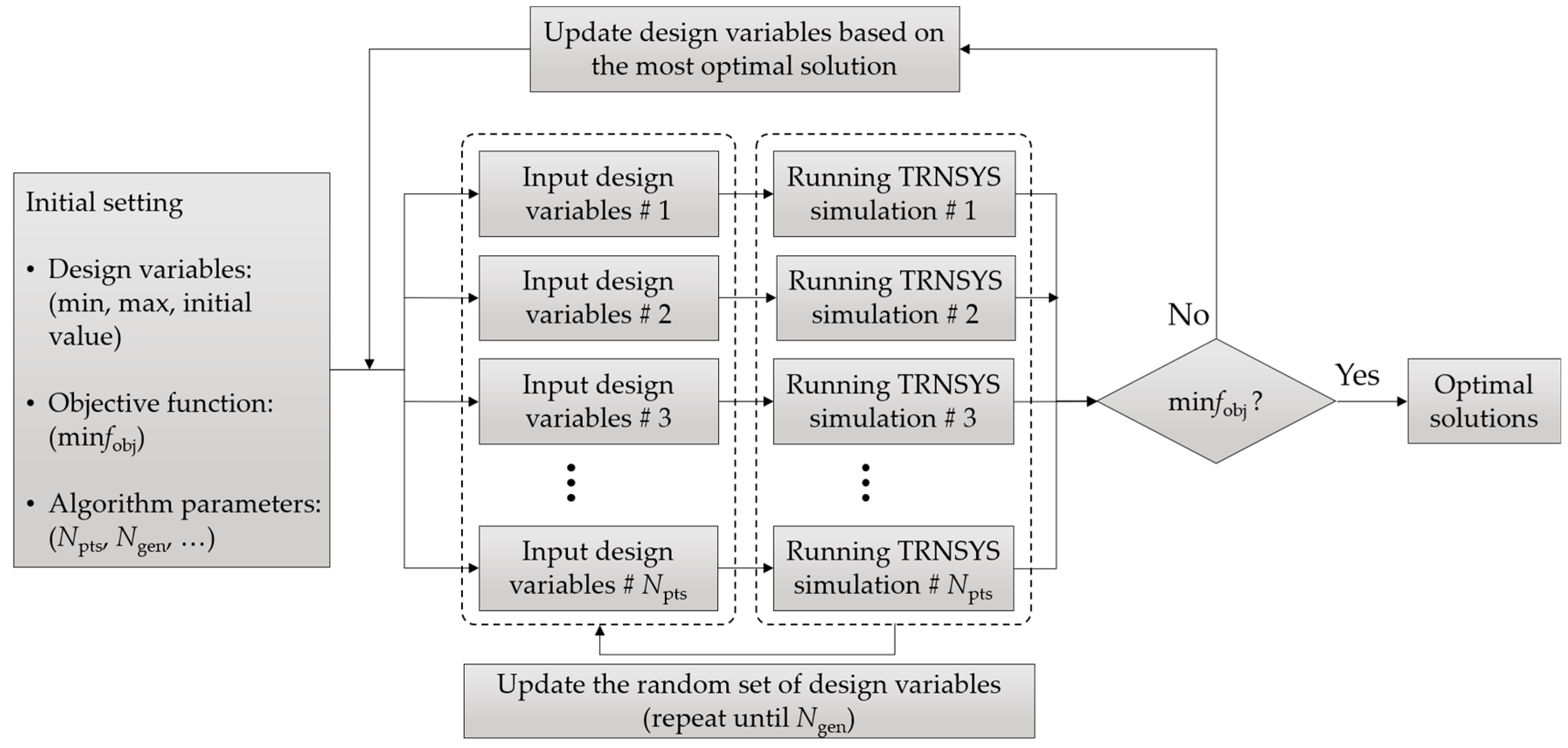
The optimization objective of the parameter calibration in the present work is to match the TRNSYS BIPV model with the in situ BIPV module by determining unknown parameters of the TRNSYS BIPV model. Thus, the particle swarm optimization (PSO) algorithm with a single objective function and without constraints was applied [32]. The PSO algorithm is a global random search algorithm for single-objective optimization. Users can set the number of particles (N_pts) and generations (N_gen). Thereafter, the algorithm searches for an optimal solution among the results provided from all the particles, moving from the first generation (N_gen = 1) to the last generation (N_gen = 50), based on the given constraints and range of design variables. The optimal solution represents a case in which the objective function is minimized. In the present study, N_pts was set to 40 and N_gen was set to 50. The flow chart for the PSO algorithm with TRNOPT is presented in Figure 5.

The same range of design variables presented in Table 3 was used for the PSO algorithm; the objective function was defined as in Equation (7), using the measured and simulated BIPV cell temperature and power production. Here, $Q_{\mathrm{total}}$ is the total radiation on the BIPV surface (W/m²), $T_{\mathrm{cell},\mathrm{sim}}$ and $T_{\mathrm{cell},\mathrm{measured}}$ indicate the BIPV cell temperature (°C), and ${\dot{E}}_{\mathrm{BIPV},\mathrm{sim}}$ and ${\dot{E}}_{\mathrm{BIPV},\mathrm{measured}}$ are the BIPV power production (kW) for the simulated and measured values, respectively. The use of the multiplier $Q_{\mathrm{total}}$ is intended to sum the differences between simulated and measured values only when beam radiation is present. Generally, the calibrated TRNSYS BIPV model with PSO optimization describes the thermal and electrical behaviors observed through in situ measurement data better than the uncalibrated model.

$$\min f_{\mathrm{obj}}=\sum _{\mathrm{start}}^{\mathrm{stop}}{Q}_{\mathrm{total}}\times \left\{\mathrm{abs}\left(T_{\mathrm{cell},\mathrm{sim}}-T_{\mathrm{cell},\mathrm{measured}}\right)+\mathrm{abs}\left({\dot{E}}_{\mathrm{BIPV},\mathrm{sim}}-{\dot{E}}_{\mathrm{BIPV},\mathrm{measured}}\right)\right\}$$

(7)

After optimization, the error between simulation and measurement results was evaluated using Equation (8), like Equation (6).

$$\mathrm{RMSE}=\sqrt{\frac{{\left(T_{\mathrm{sim}}-T_{\mathrm{mea}}\right)}^2}{N}},$$

(8)

3. Results

3.1. Results of the Parameter Sensitivity Analysis

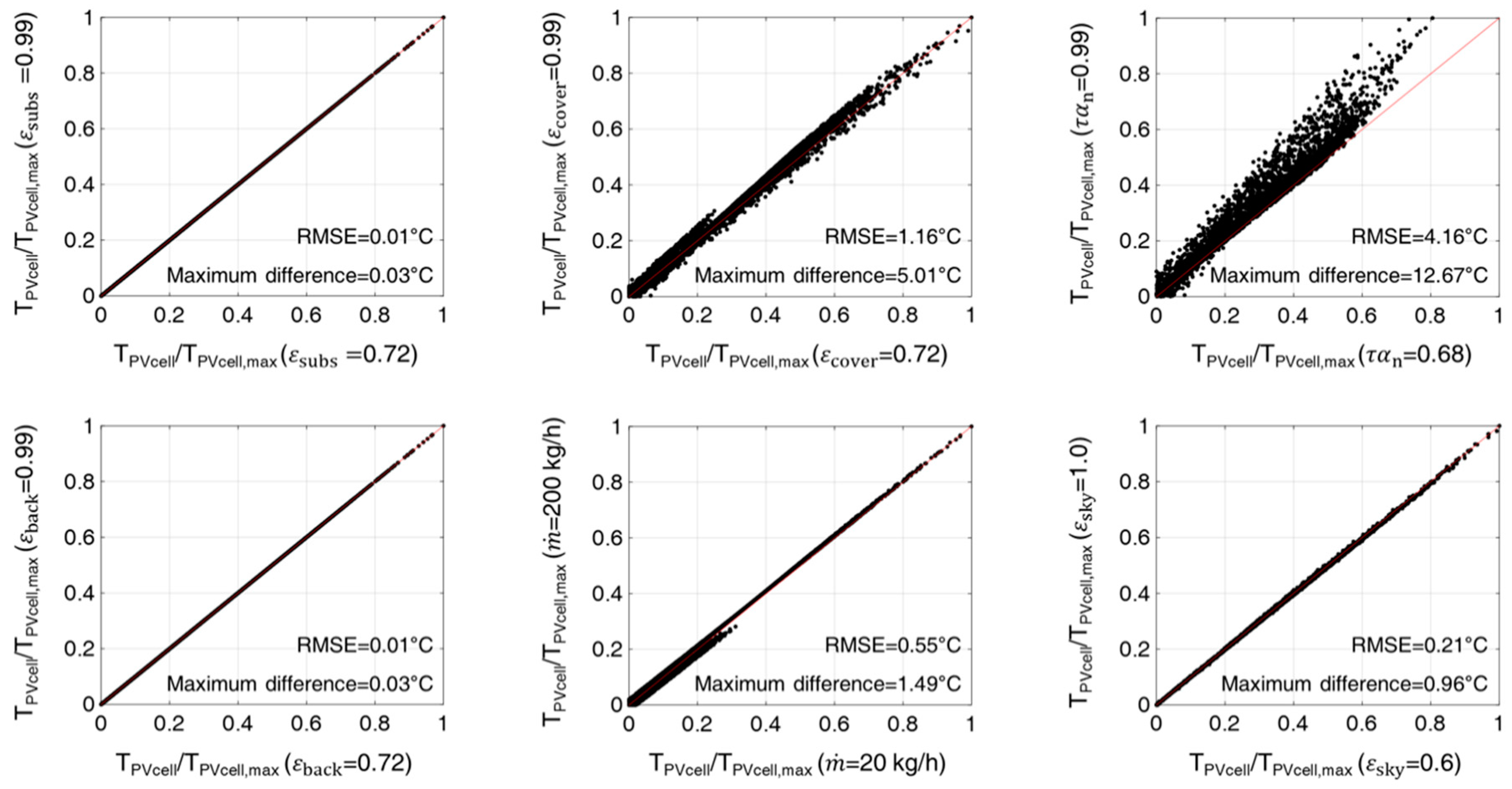
Scatter plots of the sensitivity analysis for the target variables—${\epsilon }_{\mathrm{sky}}$, ${\epsilon }_{\mathrm{cover}}$, ${\epsilon }_{\mathrm{subs}}$, ${\epsilon }_{\mathrm{back}}$, $\tau {\alpha }_{\mathrm{n}}$, and $\dot{m}$—are presented in Figure 6. The normalized BIPV cell temperatures $\left(T_{\mathrm{cell}}/T_{\mathrm{cell},\max }\right)$ were plotted for each case of the lower bound (x-axis) and upper bound (y-axis) of the target variables. The plotted points in the graphs correspond to hourly temperatures for 8760 h, but the points were obtained from two annual simulations with distinct variables of upper and lower bound variables. The scatter plots are visual representation of the degree of change in cell temperature within the range of variation of the variables to identify the variables that are sensitive to cell temperature change before calibration of the variable.

The BIPV cell temperature ($T_{\mathrm{cell}}$) is affected, with an RMSE of 0.01–4.16 °C. $T_{\mathrm{cell}}$ is rarely affected in the case of variations of 0.72–0.99 in ${\epsilon }_{\mathrm{subs}}$ and ${\epsilon }_{\mathrm{back}}$. The points are aligned on the diagonal line, so the variables of ${\epsilon }_{\mathrm{subs}}$ and ${\epsilon }_{\mathrm{back}}$ in the model are not sensitive for $T_{\mathrm{cell}}$. On the contrary, $\tau {\alpha }_{\mathrm{n}}$ exhibits the highest RMSE and a maximum difference of 12.67 °C for $T_{\mathrm{cell}}$. Other variables, such as ${\epsilon }_{\mathrm{cover}}$, ${\epsilon }_{\mathrm{sky}}$, and $\dot{m}$, exhibit RMSEs of 1.16, 0.21, and 0.55 °C, respectively; and 5.01, 0.96, and 1.49 °C in the maximum differences of $T_{\mathrm{cell}}$.

According to the results in Figure 6, ${\epsilon }_{\mathrm{cover}}$, ${\epsilon }_{\mathrm{sky}}$, $\dot{m}$, and $\tau {\alpha }_{\mathrm{n}}$ were selected as the design variables of the parameter calibration for the BIPV model, except for ${\epsilon }_{\mathrm{subs}}$ and ${\epsilon }_{\mathrm{back}}$. The eliminated variables, ${\epsilon }_{\mathrm{subs}}$ and ${\epsilon }_{\mathrm{back}}$, do not have a remarkable impact on $T_{\mathrm{cell}}$ and they show a difference of less than 10⁻³ (kW) in electrical power production.

3.2. Parameter Calibration Results for the BIPV Model

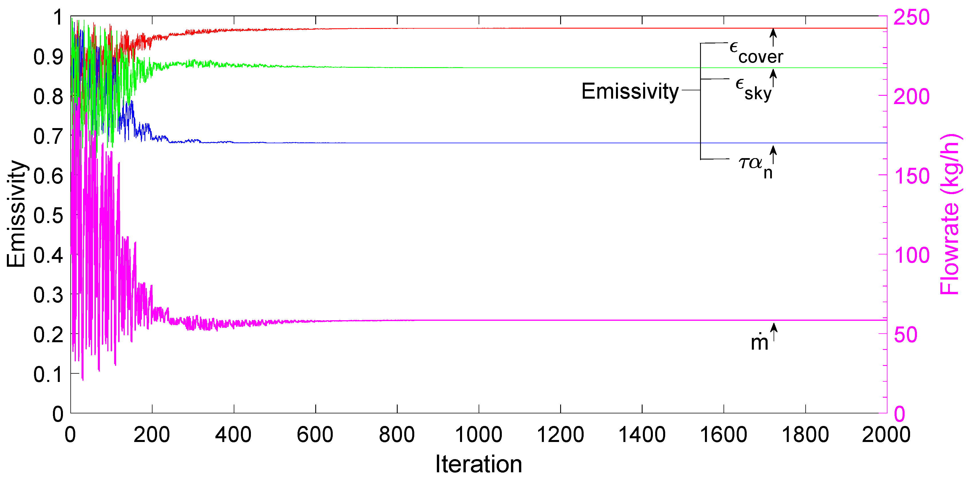
The initial values, ranges, and optimum values of the design variables used for the parameter calibration optimization are presented in

Table 4. Target variables and optimum values obtained via sensitivity analyses.

Design variables		Value				Unit
		Min.	Initial	Max.	Opt.
${\epsilon }_{\mathrm{sky}}$	Sky emissivity	0.60	0.90	0.99	0.87	-
${\epsilon }_{\mathrm{cover}}$	Cover emissivity	0.72	0.90	0.99	0.97	-
$\tau {\alpha }_{\mathrm{n}}$	Normal transmittance-absorptance	0.68	0.85	0.99	0.68	-
$\dot{m}$	Inlet flow rate of air channel	20	100	200	58.53	kg/h

. The initial values in Table 4 were changed to optimum values through approximately 2000 (N_pts × N_gen) simulations, using the PSO 50 generation.

During optimization, the initial values are arbitrarily modified within the bounds, and a set of variables to be optimized that show minimum errors are selected as starting values for the next generation. Figure 7 shows this optimization process. The iteration represents N_gen, and the plotted values for each iteration indicates a combination of the test variable with a least error among test particles. During the first 600 generations, the values fluctuated over iterations, but then they were converged to optimal values.

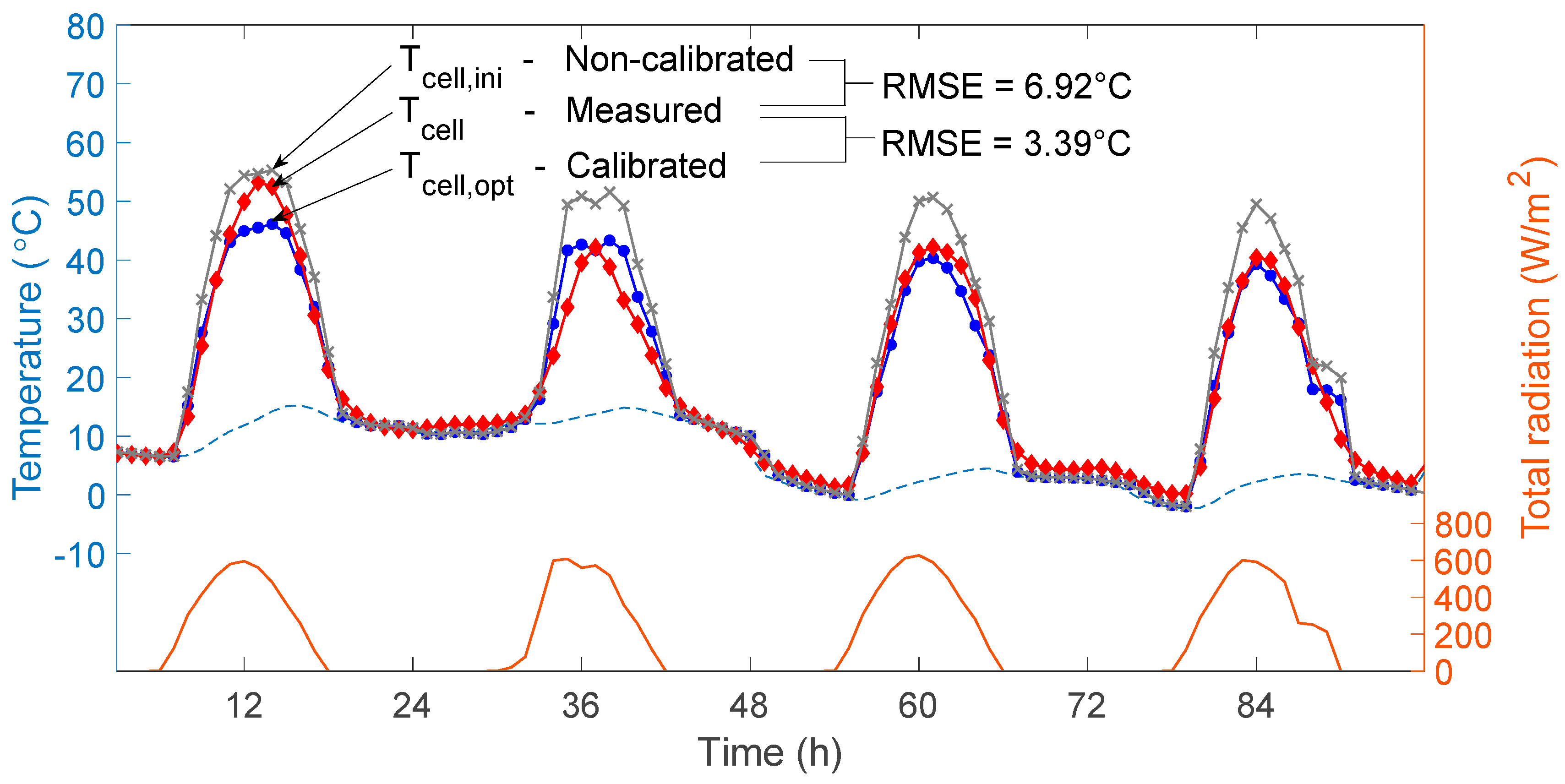
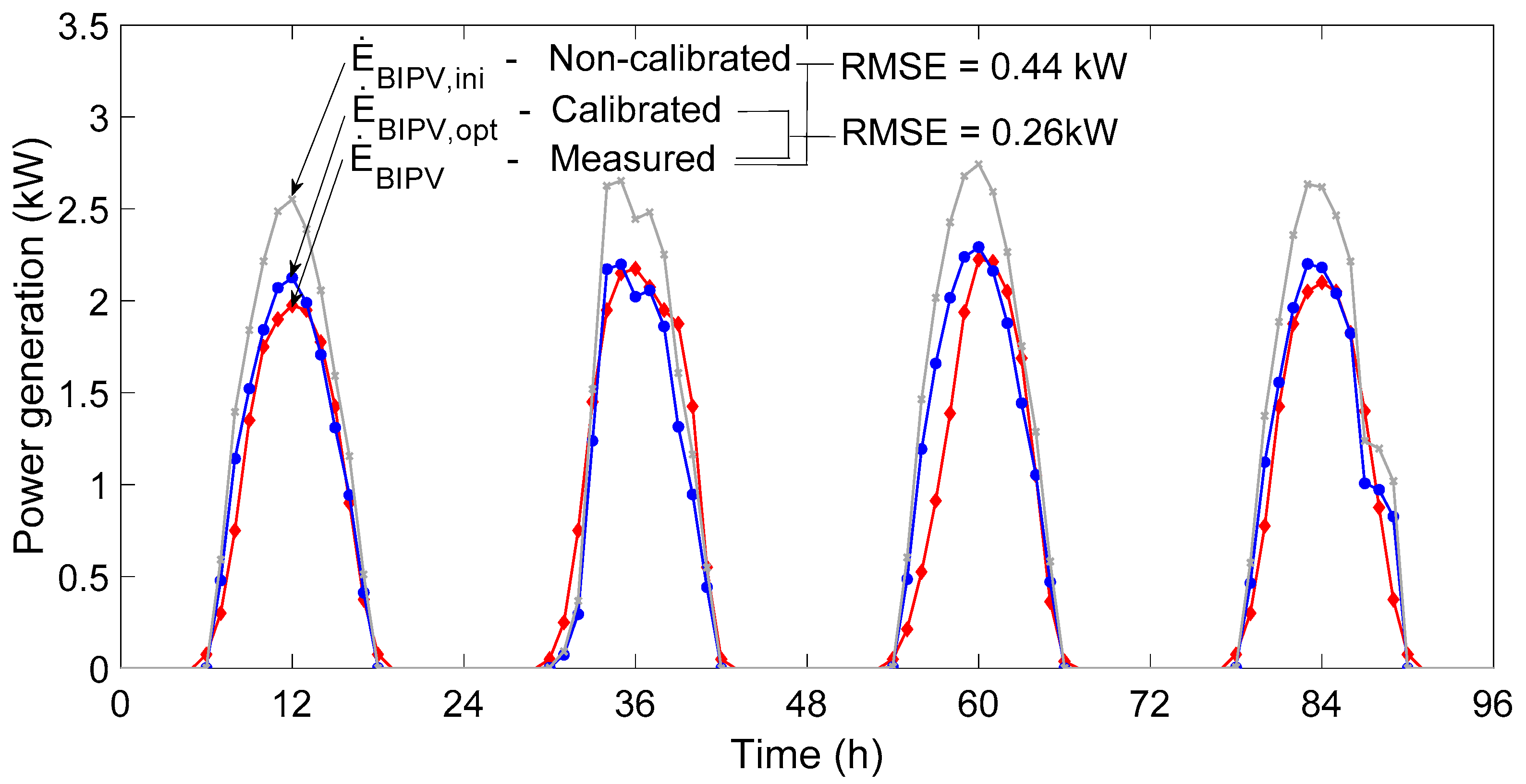
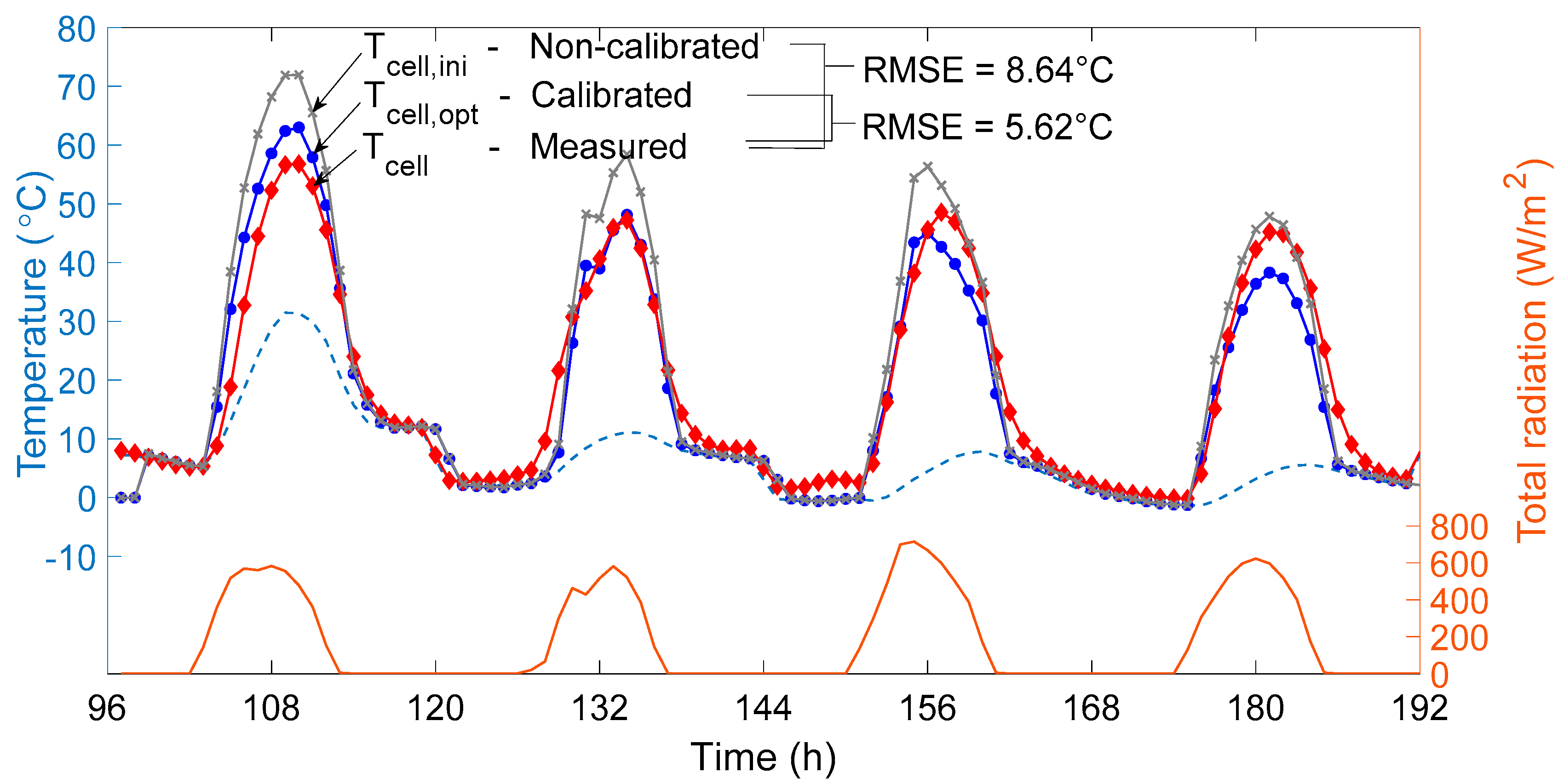
Figure 8 and Figure 9 depict the simulation results obtained using the calibrated and noncalibrated (initial) parameters. Figure 8 presents the BIPV cell temperatures. The y-axis represents temperatures while the right y-axis represents total solar radiation ($Q_{\mathrm{total}})$ on the surface, and the curve is plotted at the bottom of the figure. Figure 9 presents the BIPV power production results. The calculated power production using the BIPV simulation model represents the case obtained using 58 modules, which is obtained by multiplying the amount of power produced by a single module with the number of modules.

Prior to calibration, $T_{\mathrm{cell},\mathrm{ini}}$ had an RMSE of 6.92 °C compared to $T_{\mathrm{cell}}$, and it was reduced to an RMSE of 3.39 °C after calibration for sunlit hours. ${\dot{E}}_{BIPV,ini}$ yields an RMSE of 0.44 kW, which is also reduced to 0.26 kW using the calibrated parameters. All the noncalibrated models exhibited higher RMSEs in cell temperatures and power production, whereas the calibrated model had lower errors and a fluctuation pattern similar to that in the in situ test data. Moreover, the magnitude of calibrated cases was distinctively reduced as the calibration seemingly uses the smaller $\tau {\alpha }_{\mathrm{n}}$, i.e., the most sensitive design variable. Here, it is somewhat implied that a real value of $\tau {\alpha }_{\mathrm{n}}$ is closer to our optimum value; however, this value can be regarded as the most representative value to match the simulation and measured data in a physically acceptable range.

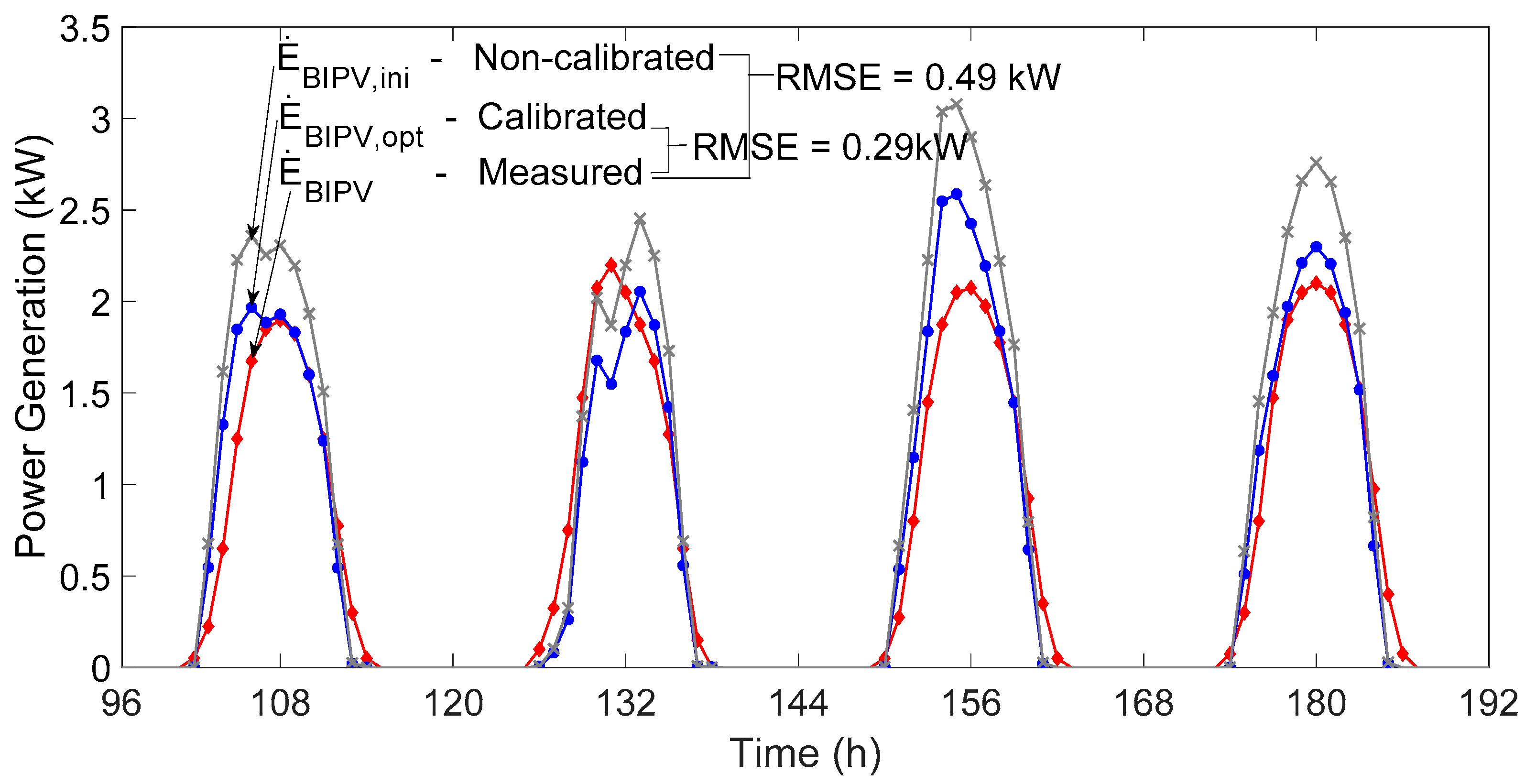
The calibrated BIPV model was evaluated by comparison with data from the remaining four days, which were not used during the optimization process. The results are shown in Figure 10 and Figure 11.

The predicted performance of the calibrated model for the last four days indicates an increased RMSE. The RMSE in the BIPV cell temperature increased from 3.39 to 5.62 °C and that in the total power production increased slightly from 0.26 to 0.29 kW. However, as shown in the figures, the calibrated model was still a better fit than the noncalibrated model.

3.3. Annual Prediction of Energy Production

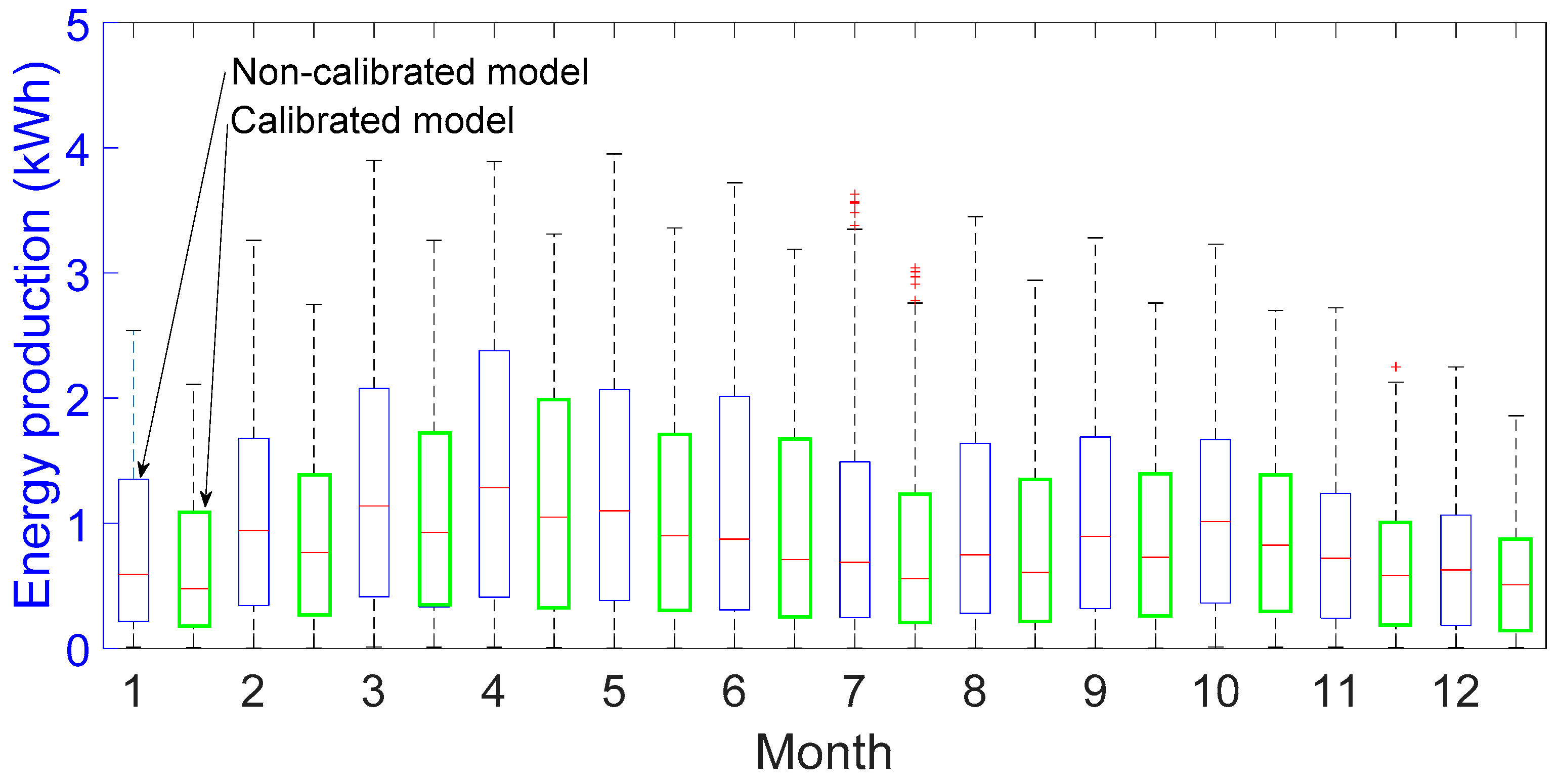
As an application example of the calibrated BIPV model, annual TRNSYS simulations were run. The second version of Typical Meteorological Year (TMY2) provided in TRNSYS was used as weather data for Seoul, and the calibrated and noncalibrated models were compared using Type 56, a building model, to give boundary temperatures to the BIPV models.

Figure 12 is a box plot that shows monthly energy production obtained by the calibrated and noncalibrated models. The BIPV energy production calculated by the calibrated model was lower than the noncalibrated model.

Table 5. Difference in BIPV energy production between calibrated and noncalibrated models.

Energy Production	Noncalibrated	Calibrated
Hourly average	1.07 kWh	0.89 kWh
Total	4750.27 kWh	3941.29 kWh

shows hourly average and annual total BIPV energy production. The annual total energy production with the calibrated model was less than the noncalibrated model by about 17%. As shown in the hourly average value, the calibrated model was also less by about 17%.

4. Conclusions

This work presents a calibration method for unknown and uncertain parameters of the BIPV simulation model in TRNSYS. Among them, the most sensitive parameters of the model, such as cover emissivity, sky emissivity, normal transmittance-absorptance, and channel flow rate, were selected via a sensitivity analysis, and these parameters were calibrated using optimum values determined by employing the PSO algorithm implemented in TRNOPT.

The calibrated BIPV simulation model exhibited an RMSE of 3.39 °C in terms of the cell temperature and an RMSE of 0.26 kW in terms of power production. These errors were lower than those for the noncalibrated model, with RMSEs of 6.92 °C and 0.44 kW for the same cases. On evaluating the predicted performance of the calibrated BIPV model, RMSEs of 5.62 °C and 0.29 kW were determined, which were still lower than those for the noncalibrated model.

Thus, this work proposes a calibration method capable of selecting sensitive parameters that need to be calibrated among parameters that are poorly defined based on available documentation and information and are not directly related to the test case. The proposed calibration method can be applied for other calibration cases, and the calibrated model presented in the work can also be used for designing and operating a similar BIPV system using proper weather data. An annual hourly simulation using that calibrated model shows a difference between that a realistic calibrated model and an initial one, and such results can be used for an economic analysis using target weather data.

To reduce the error found in this work, more parameters can be selected and calibrated that are already known to users, particularly under broader bounds. However, a projection of the calibrated model under such conditions for a long-time simulation can cause a problem of so-called out-fitting. Further work is required to investigate this issue.

References

- Alvarez-Herranz, A.; Balsalobre-Lorente, D.; Shahbaz, M.; Cantos, J.M. Energy innovation and renewable energy consumption in the correction of air pollution levels. Energy Policy 2017, 105, 386–397. [Google Scholar] [CrossRef]
- Amasyali, K.; El-Gohary, N.M. A review of data-driven building energy consumption prediction studies. Renew. Sustain. Energy Rev. 2018, 81, 1192–1205. [Google Scholar] [CrossRef]
- Chel, A.; Kaushik, G. Renewable energy technologies for sustainable development of energy efficient building. Alex. Eng. J. 2018, 57, 655–669. [Google Scholar] [CrossRef]
- Cucchiella, F.; D’adamo, I.; Gastaldi, M.; Koh, S.L. Renewable energy options for buildings: Performance evaluations of integrated photovoltaic systems. Energy Build. 2012, 55, 208–217. [Google Scholar] [CrossRef]
- Shukla, A.K.; Sudhakar, K.; Baredar, P. Recent advancement in BIPV product technologies: A review. Energy Build. 2017, 140, 188–195. [Google Scholar] [CrossRef]
- Aelenei, L.; Pereira, R.; Gonçalves, H.; Athienitis, A. Thermal performance of a hybrid BIPV-PCM: Modeling, design and experimental investigation. Energy Procedia 2014, 48, 474–483. [Google Scholar] [CrossRef] [Green Version]
- An, H.J.; Yoon, J.H.; An, Y.S.; Heo, E. Heating and cooling performance of office buildings with a-Si BIPV windows considering operating conditions in temperate climates: The case of Korea. Sustainability 2018, 10, 4856. [Google Scholar] [CrossRef] [Green Version]
- Lee, H.M.; Yoon, J.H.; Shin, U.C. Regional performance evaluation of PV System and BIPV in Korea. Autumn Conf. Acad. Present. 2014, 133–134. [Google Scholar]
- Othman, M.Y.; Ibrahim, A.; Jin, G.L.; Ruslan, M.H.; Sopian, K. Photovoltaic-thermal (PV/T) technology–the future energy technology. Renew. Energy 2013, 49, 171–174. [Google Scholar] [CrossRef]
- Bayrakci, M.; Choi, Y.; Brownson, J.R. Temperature dependent power modeling of photovoltaics. Energy Procedia 2014, 57, 745–754. [Google Scholar] [CrossRef] [Green Version]
- Yoon, J.H.; Oh, M.H.; Kang, G.H.; Lee, J.B. Annual base performance evaluation on cell temperature and power generation of c-Si transparent spandrel BIPV Module depending on the Backside Insulation Level. J. Korean Sol. Energy Soc. 2012, 32, 24–33. [Google Scholar] [CrossRef] [Green Version]
- Lee, C.S.; Lee, H.M.; Choi, M.J.; Yoon, J.H. Performance Evaluation and Prediction of BIPV Systems under Partial Shading Conditions Using Normalized Efficiency. Energies 2019, 12, 3777. [Google Scholar] [CrossRef] [Green Version]
- Yadav, S.; Panda, S.K. Thermal performance of BIPV system by considering periodic nature of insolation and optimum tilt-angle of PV panel. Renew. Energy 2020, 150, 136–146. [Google Scholar] [CrossRef]
- Goncalves, J.E.; van Hooff, T.; Saelens, D. A physics-based high-resolution BIPV model for building performance simulations. Sol. Energy 2020, 204, 585–599. [Google Scholar] [CrossRef]
- Chine, W.; Mellit, A.; Lughi, V.; Malek, A.; Sulligoi, G.; Pavan, A.M. A novel fault diagnosis technique for photovoltaic systems based on artificial neural networks. Renew. Energy 2016, 90, 501–512. [Google Scholar] [CrossRef]
- Li, S.; Joe, J.; Hu, J.; Karava, P. System identification and model-predictive control of office buildings with integrated photovoltaic-thermal collectors, radiant floor heating and active thermal storage. Sol. Energy 2015, 113, 139–157. [Google Scholar] [CrossRef]
- Agathokleous, R.A.; Kalogirou, S.A. Part I: Thermal analysis of naturally ventilated BIPV system: Experimental investigation and convective heat transfer coefficients estimation. Sol. Energy 2018, 169, 673–681. [Google Scholar] [CrossRef]
- Debbarma, M.; Sudhakar, K.; Baredar, P. Thermal modeling, exergy analysis, performance of BIPV and BIPVT: A review. Renew. Sustain. Energy Rev. 2017, 73, 1276–1288. [Google Scholar] [CrossRef] [Green Version]
- Hachana, O.; Tina, G.M.; Hemsas, K.E. PV array fault DiagnosticTechnique for BIPV systems. Energy Build. 2016, 126, 263–274. [Google Scholar] [CrossRef]
- Vuong, E.; Kamel, R.S.; Fung, A.S. Modelling and simulation of BIPV/T in EnergyPlus and TRNSYS. Energy Procedia 2015, 78, 1883–1888. [Google Scholar] [CrossRef] [Green Version]
- Yang, T.; Athienitis, A.K. A study of design options for a building integrated photovoltaic/thermal (BIPV/T) system with glazed air collector and multiple inlets. Sol. Energy 2014, 104, 82–92. [Google Scholar] [CrossRef]
- Huang, C.Y.; Chen, H.J.; Chan, C.C.; Chou, C.P.; Chiang, C.M. Thermal model based power-generated prediction by using meteorological data in BIPV system. Energy Procedia 2011, 12, 531–537. [Google Scholar] [CrossRef] [Green Version]
- Liao, L.; Athienitis, A.K.; Candanedo, L.; Park, K.W.; Poissant, Y.; Collins, M. Numerical and experimental study of heat transfer in a BIPV-thermal system. Sol. Energy Eng. 2007, 129, 423–430. [Google Scholar] [CrossRef]
- Liu, B.Y.H.; Jordan, R.C. The Interrelationship and of Direct, Diffuse and Characteristic Distribution Total Solar Radiation. Sol. Energy 1960, 4, 1–19. [Google Scholar] [CrossRef]
- Jeon, B.K.; Kim, E.J.; Shin, Y.; Lee, K.H. Learning-based predictive building energy model using weather forecasts for optimal control of domestic energy systems. Sustainability 2019, 11, 147. [Google Scholar] [CrossRef] [Green Version]
- Klein, S.; Beckman, A.; Mitchell, W.; Duffie, A. TRNSYS 17-A TRansient SYstems Simulation Program; Solar Energy Laboratory, University of Wisconsin: Madison, WI, USA, 2011. [Google Scholar]
- Mondol, J.D.; Yohanis, Y.G.; Norton, B. Comparison of measured and predicted long term performance of grid a connected photovoltaic system. Energy Convers. Manag. 2007, 48, 1065–1080. [Google Scholar] [CrossRef]
- Evangelisti, L.; Guattari, C.; Asdrubali, F. On the sky temperature models and their influence on buildings energy performance: A critical review. Energy Build. 2019, 183, 607–625. [Google Scholar] [CrossRef]
- Fernández, M.; Eguía, P.; Granada, E.; Febrero, L. Sensitivity analysis of a vertical geothermal heat exchanger dynamic simulation: Calibration and error determination. Geothermics 2017, 70, 249–259. [Google Scholar] [CrossRef]
- Tang, R.; Etzion, Y.; Meir, I.A. Estimates of clear night sky emissivity in the Negev Highlands, Israel. Energy Convers. Manag. 2004, 45, 1831–1843. [Google Scholar] [CrossRef]
- Wetter, M. GenOpt-A generic optimization program. In Proceedings of the Seventh International IBPSA Conference, Rio de Janeiro, Brazil, 13–15 August 2001; pp. 601–608. [Google Scholar]
- Bai, Q. Analysis of particle swarm optimization algorithm. Comput. Inf. Sci. 2010, 3, 180. [Google Scholar] [CrossRef] [Green Version]
Figure 1.
Concept diagram of the proposed methodology for developing a calibrated model.
Figure 2.
Southern elevation of the main building and installation location of the target C-Si BIPV modules.
Figure 3.
Measurement locations for BIPV modules installed on the spandrel of the target building.
Figure 4.
Thermal network of TRNSYS type 567 (BIPV simulation model).
Figure 5.
Particle swarm optimization (PSO) algorithm with TrnOpt and TRNSYS.
Figure 6.
Scatter plots of sensitivity analysis for unknown parameters regarding BIPV cell temperatures.
Figure 7.
Optimization process results using GenOpt.
Figure 8.
Results of calibrated and noncalibrated models for BIPV cell temperatures (first four days).
Figure 9.
Results of calibrated and noncalibrated models for BIPV power production (first four days).
Figure 10.
Temperature evaluation of calibrated and noncalibrated models for unused in situ test data (last four days).
Figure 11.
Power production of calibrated and noncalibrated models for unused in situ test data (last four days).
Figure 12.
Monthly power generation differences between calibrated and noncalibrated models.