A Novel Approach to Enhance the Generalization Capability of the Hourly Solar Diffuse Horizontal Irradiance Models on Diverse Climates

Abstract

Solar radiation data is essential for the development of many solar energy applications ranging from thermal collectors to building simulation tools, but its availability is limited, especially the diffuse radiation component. There are several studies aimed at predicting this value, but very few studies cover the generalizability of such models on varying climates. Our study investigates how well these models generalize and also show how to enhance their generalizability on different climates. Since machine learning approaches are known to generalize well, we apply them to truly understand how well they perform on different climates than they are originally trained. Therefore, we trained them on datasets from the U.S. and tested on several European climates. The machine learning model that is developed for U.S. climates not only showed low mean absolute error (MAE) of 23 W/m², but also generalized very well on European climates with MAE in the range of 20 to 27 W/m². Further investigation into the factors influencing the generalizability revealed that careful selection of the training data can improve the results significantly.

1. Introduction

Building performance simulation tools such as EnergyPlus [1], TRNSYS [2] etc., requires detailed information on the magnitudes of diffuse and direct components of solar radiation for prediction of energy consumption [3]. The knowledge of these components also enables us to simulate light behavior in complicated environments and render High-dynamic-range (HDR) photorealistic images using lighting visualization tools such as Radiance [4] that are invaluable for designers, architects and daylight simulation [5] researchers alike. Sizing and configuration of solar energy systems such as solar thermal collectors and photovoltaic cells entail reliable solar radiation measurements. However, measuring both these components simultaneously can be expensive as measuring the direct component requires a pyrheliometer along with a solar tracker to track the sun at all times and similarly a shadow band with a pyranometer is needed for the diffuse component. Global solar radiation, which includes both these components, is rather simple and commonly measured not only in meteorological stations but also in smaller local weather stations. A cost-effective approach to obtain diffuse and direct components is to either use various correlations, or develop prediction models based on global solar radiation along with other meteorological parameters.

Several studies evaluating the diffuse component started to appear in the 1960s based on the work of Liu and Jordan [6], which utilised curve fitting models with polynomial terms. Most of the models that are based on Liu and Jordan [6], like Orgill and Hollands [7], Erbs et al. [8], Reindl et al. [9] etc., are based on the relationship between the clearness index ($k_t$) and diffuse fraction ($F_d$), where $F_d$ is the ratio between diffuse ($D_h$) and Global horizontal irradiance ($G_h$) and $k_t$ is the ratio between Global horizontal irradiance ($G_h$) and extraterrestrial solar irradiance ($G_o$). Although they are based only on this relationship, their models differed as they developed them on different datasets. Therefore, these models are to be curve fitted frequently to adapt to the new datasets, which makes the generalization of these models very difficult.

Recent studies have shown that machine learning approaches have made promising strides in this field. Boland et al. [10] and Ruiz-Arias et al. [11] developed logistic and regression models respectively for diffuse fraction prediction. Soares et al. [12] modeled a perceptron neural-network for São Paulo City, Brazil, to estimate hourly values of the diffuse solar-radiation, which perfomed better than the existing polynomial models. Similar studies conducted by Elminir et al. [13] and Ihya et al. [14] in Egypt and Morocco respectively also supports the fact that neural networks are better predictors than other linear regression models. A recent review by Berrizbeitia et al. 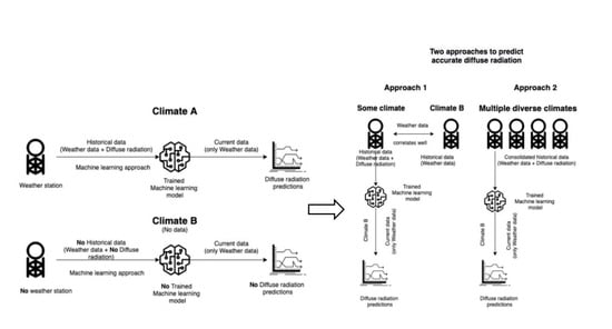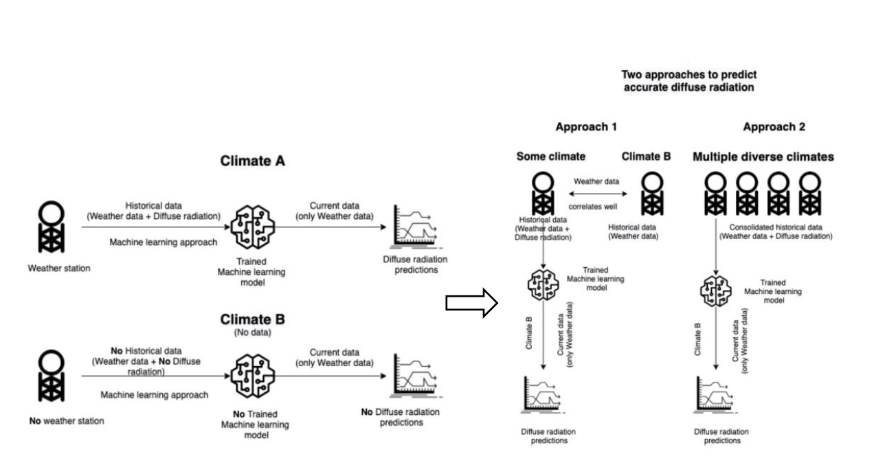[15] also perfectly summarized both empirical and machine learning based models, but many of these models have not explored the possibility of the generalization of these models on different climates. In most of these models, the training data and testing data is from the same climates. Most of the regression models can show exceptional performance in this type of experimental setup, but they fail to show the same performance on different climates. Most of the climates do not have historical data to develop good regression models, but there might be some climates around it which may be abundant in such data. The idea of our research is to harvest this data to develop models and reliably use it to predict for climates that lack historical data.

This motivated us to explore the contemporary ways of exploiting the data using machine learning algorithms, as they learn to adapt and produce reliable and repeatable results. While experimenting with several models we also found that their performance is affected by their training datasets. Therefore, we bring forward to the readers our observations and present some recommendations to improve the generalizing capability of these models.

In Section 2, we first give a brief introduction of all the predictive models compared in this study along with finetuning techniques that improve the performance of these models. The polynomial model of Erbs et al. is chosen as a baseline to compare against other machine learning models (linear regression, decision tree, random forests, gradient boosting and XGBoost, and an artificial neural network). The workflow of this study is to first find the best performing approaches by comparing them on the same datasets and then check for their generalizability on a third unseen dataset. Secondly, the best performing approaches are tested with completely different datasets to see if they can reliably make similar predictions and analyze what factors would affect their performance. To make the results reproducible all datasets used in this study along with their locations and data preprocessing techniques are mentioned in Section 3.

Explored hyperparameter configurations of the machine learning models and thus achieved best configurations through finetuning are described in Section 4. Here we also present our findings in two parts. First we present the performance of all the predictive models based on the most commonly used metrics for all the datasets considered in this study along with their generalization capability. Secondly we select the best performing approaches from the first part and train them with U.S. climates and tested them on European climate to check their reliability. Finally, for each part we discuss our findings and present our recommendations on how to select the training datasets to achieve better performing models.

2. Predictive Models

2.1. Polynomial Model (Erbs et al. Model)

Dervishi and Mahdavi [16] studied eight polynomial models, based on their prior reported performance and concluded that the best performing polynomial models were those of [7,8,9]. As all three of these models perform equally good, we decided to compare our machine learning models with only the Erbs et al. model.

Erbs et al. proposed a relation between the clearness index ($k_t$) and diffuse fraction ($F_d$). This model is based on the data from five U.S. weather stations. The diffuse fraction $F_d$ with model coefficients (see

Table 1. The Erbs et al. model’s coefficients for different datasets.

Dataset	a	b	c	d	e	f	g	h
Original (U.S)	1.00	0.09	0.9511	0.1604	4.39	16.64	12.34	0.165
Mannheim	1.00	0.04	0.0332	−8.5086	−23.47	−19.68	−4.06	0.259
Ensheim	0.95	0.12	0.3098	−5.4846	−14.62	−9.44	0.04	0.276

) is given by the following set of equations:

• $if{k}_t\le 0.22then:$

  $$F_d=a-b{k}_t$$

  (1)
• $elseif0.22<k_t\le 0.8then:$

  $$F_d=c-d{k}_t+e{k}_t^2-f{k}_t^3+g{k}_t^4$$

  (2)
• $elseif{k}_t>0.8$

  $$F_d=h$$

  (3)

  where,

  $$k_t=\frac{G_h}{G_o·sin\alpha }$$

  (4)

  and

  $$F_d=\frac{D_h}{G_h}$$

  (5)

  $$G_o=G_{sc}·\left(1+0.33cos\frac{360d}{365}\right)·cos{\theta }_z$$

  (6)

2.2. Machine Learning Models

Machine learning algorithms are a collection of statistical methods that can be trained to predict and analyze trends. These statistical models, which drew good inferences from weather data led to finding more generalizable predictive patterns. Machine learning models that find these patterns in the data by learning from labeled data are called supervised learning models. In this paper we will discuss briefly few supervised learning models such as linear regression, decision trees, random forests, gradient boosting and XGBoost.

2.2.1. Linear Regression

Linear regression [17] is used to establish the relationship between dependent and independent variables using a linear approach. When the independent variables are more than one, it is called multiple linear regression. It has been studied rigorously and used extensively in several practical applications. In this study, we adopted the least squares approach to fit the model.

2.2.2. Decision Trees

Decision trees [18] are non-parametric methods that build regression or classification models in the form of trees. Decision trees predict the target value by learning simple decision rules by inferring data features. A decision tree is built top-down by breaking down a dataset recursively into smaller datasets based on decision rules called decision nodes. The decisions on the target values are represented by leaf nodes. Therefore, the final tree appears as a set of several decision nodes and leaf nodes.

2.2.3. Random Forests

Random forests [19] use decision trees as building blocks to build more powerful prediction models. The algorithm is an ensemble of decision trees with nearly the same parameters as a decision tree, but considers only a random subset of features for splitting a node, thus introducing additional randomness to the model, while growing the trees. All the decision trees are modeled based on a different subsample of data and each observation of the subsample is chosen with replacement. Thus, this technique takes many uncorrelated learners to make a final model with reduced variance and improved performance.

2.2.4. Gradient Boosting

The idea of combining several weak learners intelligently into a strong learner is called boosting. Gradient boosting [20] is an ensemble learning approach, where we build an ensemble of regressors incrementally in several steps. At each step a new sub-model is added, that tries to compensate for the residuals (errors) made by the previous sub models. These sub models are fairly simple and decision trees are usually the classic choice. The intuition behind the gradient boosting algorithm is to repetitively leverage the patterns from the residuals and strengthen a model with weak predictions to make it a strong predictor. The training of the predictor stops at the stage where residuals do not have any pattern that could be modeled.

2.2.5. XGBoost

XGBoost (“Extreme Gradient Boosting”), a variant of gradient boosting, implemented in library XGBoost by Chen and Guestrin [21], is also used in this study. It is an optimized distributed gradient boosting implementation designed to be more efficient, flexible and portable than existing gradient boosting implementation. Unsurprisingly, it is recognized as the best approach by the European Organization for Nuclear Research (CERN) [22] for classifying signals from the Large Hadron Collider. Unlike gradient boosting, XGBoost uses a more regularized model formalization to control overfitting and thus achieves better performance.

2.2.6. Neural Networks

Artificial neural networks (ANN) [23], a branch of machine learning, has attracted a great deal of attention in recent years. In this study, we will discuss building a deep learning neural network, a more advanced form of neural network which is wider and deeper than traditional neural networks, that produces more accurate predictions of hourly diffuse fraction from a variety of meteorological data. It shows that by increasing hidden layers, the need for feature extraction can be avoided, which was a crucial step in previously developed neural network models.

2.3. Basics of Neural Networks

Neural networks (NNs) are inspired by biological neural networks and can perform certain tasks by learning from examples, without the need to program for each individual task. They are used in a wide range of applications such as speech and image recognition, computer vision, machine translation, medical diagnosis and even board games. Feed-forward multi-layered perceptrons (MLPs) are the most common neural networks which are simple but can solve complex problems. A deep neural network (DNN) is an MLP with multiple hidden layers, which avoids the manual process of handcrafted feature engineering by learning feature significance automatically. With the introduction of high power Graphical Processing Units (GPUs) and Compute Unified Device Architecture (CUDA) framework, neural networks can now be easily widened and deepened without much concern for the memory and processing power.

The neural network has several neurons in the input layer, each one representing a feature (input) and several hidden layers with a variable number of neurons and an output layer with neurons, each representing an output. Every neural network has a set of weights, bias and activation functions. The input that enters the neuron is multiplied by weights, which are randomly initialized and then updated during the training process. At the end of the training, features with higher significance achieve higher weightage and vice versa. An activation function translates the linear combination of weight multiplied inputs and bias to output value. The bias added here to the weight multiplied inputs acts as a range shifter for output from the activation function. The data input is transformed by passing through several hidden layers to predict the output as close as possible to the actual value. The objective is to reduce the error (difference between output and actual value) using a cost function, thus increasing the accuracy of prediction. The randomly assigned weights are now updated with backpropagation [24], where the error is fed back to the network along with the gradient of the cost function. To generalize the network, the data is sent in chunks of equal size called batches. A single training iteration with all the batches performing the forward and backward propagation is called an Epoch. To minimize the cost function of the network, an optimizing algorithm such as gradient descent is used. It finds the local minimum of the cost function by taking proportional steps based on the learning rate.

2.4. Fine Tuning

To achieve the best results from the machine learning models and neural networks, fine tuning is essential. Fine-tuning or hyperparameter optimization finds the right set of weights, activation functions, learning rates and different constraints that yield an optimal model, which minimizes the loss of cost function on a given validation data. Even the Erbs et al. model is adapted using curve-fitting methods for all datasets (see Table 1).

2.4.1. Grid Search with Cross Validation

Grid search [25,26] or parameter sweep is traditionally used for optimizing hyperparameters. It exhaustively searches through a parameter space, a subset specified manually over the hyperparameter space of the learning algorithm. Usually a grid search algorithm requires a performance metric such as cross-validation, which estimates the accuracy of the prediction algorithm in practice and how well the algorithm generalizes on an independent data set. Cross-validation involves partitioning the dataset into k subsets, performing the training on any k-1 subsets and validating on the remaining subset. This is repeated with a different set of k-1 subsets in multiple rounds until all the combinations are exhausted. Multiple rounds of cross-validation with different partitions reduce the variability, and the results from all the rounds are combined or averaged to give an estimate of the model’s predictive performance.

2.4.2. Overfitting

An overfitted model performs well on training data but performs poorly on validation data because the model begins to memorize training data after a certain number of epochs/passes and fails to generalize the trend when testing unseen data. This can happen for several reasons such as if the model contains more parameters than can be justified by the data, or non-conformity of the data shape with the model structure, or higher model loss when compared to the expected level of noise and sometimes even error-prone data. There are several techniques to reduce the chance of overfitting such as early stopping, dropout regularization and pruning.

2.4.3. Early Stopping

Early stopping is a regularization technique used in iterative training methods such as gradient descent, to avoid overfitting. It allows the model to better fit the training data with each iteration until a certain point, where the model’s performance on data outside the training set does not improve anymore. Certain rules in early stopping guide the number of iterations that can be run before the model starts to overfit. One such method is validation-based early stopping [27], where rules are set to split the original training set into a new training set and a validation set and the loss on the validation set is used as a proxy to determine the beginning of overfitting. Validation loss is calculated at the end of every epoch, and when it does not show any improvement after certain epochs, training stops at this point and the weights of the network in the previous step is used.

2.4.4. Dropout Regularization

Dropout regularization [28,29] reduces overfitting by randomly omitting, certain number of feature detectors or neurons on each training case. As a result, each neuron learns to detect a feature in general, within the vast combination of contexts it operates, rather than developing complex co-adaptations with several other specific feature detectors.

2.4.5. Pruning

Pruning, a term often associated with decision trees, is a technique to reduce overfitting by reducing the size of the decision trees by removing the least powerful parts of the tree. The regression tree algorithm recursively partitions the data into smaller subsets until those final subsets are homogeneous in terms of the outcome variable. This often leads to final subsets (leaves) each consisting of only one or a few data points, which implies the data is learned exactly by the tree and any new data point that differs slightly might not be well predicted. Such instances can be avoided by pruning back the tree until the cross validated error is minimized.

3. Methodology

3.1. Data Collection

In this paper, a total of fourteen datasets collected from 3 different networks of ground-based stations were used. The first network of stations is from Germany, operated by Deutscher Wetterdienst (DWD [30]). The weather stations considered in this network are Mannheim, Ensheim (Saarbrücken) and Weinbiet (Neustadt) are shown in

Table 2. Deutscher Wetterdienst (DWD) weather stations in Germany and their locations.

Weather Station	ID	Latitude	Longitude	Elevation (m)	Timezone	Sample Size
Mannheim	05906	49.50	8.55	98	Europe/Berlin	103,672
Ensheim (Saarbrücken)	04336	49.21	7.11	320	Europe/Berlin	103,246
Weinbiet (Neustadt)	05426	49.37	8.12	553	Europe/Berlin	95,422

. The samples in these datasets are of 10-min intervals and can be downloaded via its FTP website. The second network of stations belong to the surface radiation budget network (SURFRAD) [31] in U.S., where the data is available at 1-min resolution for all seven stations shown in

Table 3. SURFRAD weather stations in the U.S. and their locations.

Weather Station	ID	Latitude	Longitude	Elevation (m)	Timezone	Sample Size
Bondville	BON	40.05	−88.37	213	America/Chicago	371,015
Desert Rock	DRA	36.62	−116.02	1007	America/Los Angeles	376,967
Fort Peck	FPK	48.30	−105.10	634	America/Denver	299,835
Goodwin Creek	GWN	34.25	−89.87	98	America/Chicago	369,620
Penn State University	PSU	40.72	−77.93	376	America/New York	376,967
Sioux Falls	SXF	43.73	−96.62	473	America/Chicago	374,522
Table Mountain	TBL	40.12	−105.23	1689	America/Denver	382,237

. The data from the network can be accessed via a simple python script available on their website. The third set of stations are from Baseline Solar Radiation Network (BSRN) [32] shown in

Table 4. BSRN weather stations in Europe and their locations.

Weather Station	ID	Latitude	Longitude	Elevation (m)	Timezone	Sample Size
Cabauw, The Netherlands	CAB	51.97	4.93	0	Europe/Amsterdam	185,812
Carpentras, France	CAR	44.08	5.06	100	Europe/Paris	179,604
Cener, Spain	CNR	42.82	−1.60	471	Europe/Madrid	173,698
Palaiseau, France	PAL	48.71	2.21	156	Europe/Paris	143,563

, where the data is also available at 1-min intervals. The data access is available via both FTP and PANGAEA websites [33]. Apart from these datasets two publicly available satellite-derived diffuse fractions were used for prediction alongside the data from SURFRAD and BSRN networks. National Solar Radiation Database (NSRDB) [34] modeled using a physical solar model (PSM) is available at 30-min resolution covering most of the U.S. with a spatial resolution of 0.04°. NSRDB data can be accessed via a simple python script available at the NREL website. This data was interpolated to 1-min interval and used along with SURFRAD data for prediction. Similarly Copernicus Atmospheric monitoring service—radiation service (CAMS-RAD) [35] was used along with BSRN data. CAMS-RAD data is publicly available at their website with a spatial extent of −66° to 66° in both latitudes and longitudes.

3.2. Data Preparation

The data is preprocessed to improve its quality. Several criteria have been enforced to remove those samples in the data which were wrong and violated physical limits. Machine learning models usually need data scaled to a standard form, to keep the variance of different features in the same range, especially to validate on unseen data. Therefore all the input features are standardized using quantile transformation [26] available in the scikit-learn library for python. This transforms the features to follow the uniform distribution and speed up the convergence of optimization algorithms such as stochastic gradient descent [36].

3.3. Experimental Design

This study is divided into two parts:

• In the first part, all the predictive models described in Section 2 are first trained on preprocessed datasets of Mannheim and Ensheim (both in Germany) with historical data between the years 2013–2016. During training, all the models are tuned for their best performance using different techniques defined Section 2.4. All the models are then validated against respective climate datasets from 2017 to evaluate their performances usings metrics defined in Section 3.4. These models are then tested for their capability of generalization on a third dataset of Weinbiet (Germany) on 2017 data. The aim here is to identify which approaches generalize well and apply those methodologies in the next part.
• In the second part, the main goal is to ascertain that the best performing approaches from the previous study are in fact generalizable on completely different training and test sets. To keep the experiment simple only the two best performing approaches are considered here. The training data sets are chosen from 7 climates in the U.S. from the year 2015. A predictive model for the U.S. is developed with the consolidated data from all the 7 climates. For a comparision, individual predictive models are also developed for each climate seperately. Fine tuning techniques for respective approaches are applied to improve their performance before they are tested on test datasets. The models are first validated on their respective climates with data from the year 2016. Once these models show good validation performance, then they are tested against four climates from Europe to determine their extent of generalization. The test data chosen is from the year 2016.
• Finally we derive conclusions based on model performances with different training datasets, especially how they perform on unseen datasets in Germany when trained with local (Germany) and international (U.S.) training sets.

3.4. Evaluation Metrics

The performance of all the predictive models is assessed based on these four metrics: normalized Root Mean Squared Error (nRMSE), normalized Mean Biased error (nMBE), Root Mean Squared Error (RMSE), and Mean Absolute Error (MAE). They are defined as follows,

$$\begin{array}{cc}\hfill nRMSE& ={\displaystyle \frac{\sqrt{\frac{1}{N}{\displaystyle \sum _{i=1}^N}{(p_i-m_i)}^2}}{\frac{1}{N}{\displaystyle \sum _{i=1}^N}{m}_i}}\hfill \end{array}$$

(7)

$$\begin{array}{cc}\hfill nMBE& ={\displaystyle \frac{{\displaystyle \sum _{i=1}^N}(p_i-m_i)}{{\displaystyle \sum _{i=1}^N}{m}_i}}\hfill \end{array}$$

(8)

$$\begin{array}{cc}\hfill RMSE& =\sqrt{\frac{1}{N}{\displaystyle \sum _{i=1}^N}{(p_i-m_i)}^2}\hfill \end{array}$$

(9)

$$\begin{array}{cc}\hfill MAE& =\frac{1}{N}{\displaystyle \sum _{i=1}^N}\left|p_i-m_i\right|\hfill \end{array}$$

(10)

where $m_i$ is the ith measured value, $p_i$ is the predicted value, $\overline{m}$ is the mean of the measured values and N is the number of data samples.

4. Results and Discussion

4.1. Tuning Results

Prior to the test for generalizability, the models are finetuned to give improved validation performance. Grid search is performed on the machine learning models based on several hyperparameters. Decision trees, random forests, gradient boosting trees, and XGBoost trees are each grid searched at several depths starting from 4 until 15. Random forests are tested with several different numbers of trees starting from 50 until 250. When it comes to boosting stages of gradient boosting and XGBoost, they are also grid-searched starting from 50 until 250 stages. Additionally, a few hyperparameters are searched in XGBoost models such as the learning rate (from 0.05 to 0.15), subsample ratio (from 0.08 to 0.1 ) and L2 regularization [37] of weights (from 0.80 to 1). The hyperparameters for the machine learning models can be seen in

Table 5. Parameters for machine learning algorithms.

Model	Parameters	XGB	GB	RF	DT
Mannheim	Estimators (trees)	80	150	300	NA
	Max depth	6	4	10	8
Ensheim	Estimators (trees)	80	80	150	NA
	Max depth	5	5	9	8
U.S.	Estimators (trees)	80	-	-	-
	Max depth	4	-	-	-

.

The neural networks chosen in this study for both parts are similar. They are feed forward MLPs and have 11 features (Mannheim and Ensheim) and 10 features (U.S), 6 hidden layers (shown in

Table 6. Model summary of neural networks.

Hidden Layer	# Neurons	Activation Functions
		Ensheim	Mannheim	U.S
1	1024	elu	elu	elu
2	512	elu	elu	elu
3	256	elu	elu	elu
4	128	sigmoid	elu	elu
5	64	elu	tanh	sigmoid
6	32	sigmoid	sigmoid	sigmoid

) and the output with a single neuron gives diffuse fraction ($F_d$) with sigmoid as the activation function. All hidden layers except the last hidden layer have the dropout regularization added. The dropout fraction is set to 0.3.

Neural networks are implemented using Keras library [38] and Grid search from Scikit learn [26] is implemented to search for the best combination of hyperparameters.

The choice of activation functions for all the hidden layers are ELU (Exponential Linear unit) [39], sigmoid [40] and tanh. Early stopping is implemented with validation loss as a proxy to stop training automatically after 10 epochs in the case of no improvement. A model checkpoint is implemented to save the best models at every epoch. The loss function used is mean square error and the optimizer ‘Adam’ [41] is chosen, as it has shown some good results with the default configuration of learning parameters. Table 6 shows the combination of activations functions obtained by grid search for hidden layers in Ensheim, Mannheim and U.S. models.

4.2. First Study

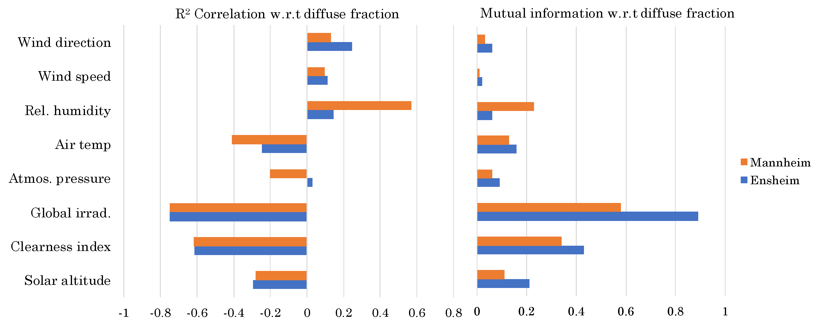
Before the predictive models are trained, a small analysis of the data is performed to see how the input features influence the output, i.e., diffuse fraction. Mutual information(MI) [42] and the R² correlation [43] of the input features with respect to the output $F_d$ is used for this analysis. Figure 1 ascertains the significance of each input feature.

MI is a measure of mutual dependence between the variables, whereas R² correlation gives a proportion of variance that the independent variable predicts from a dependent variable. It can be observed that diffuse fraction is primarily dependent on global horizontal irradiance and the clearness index, but the other parameters also show considerable but varying influences in both climates.

Since the machine learning models can easily handle these minimal number of input features, we considered all the features without discrimination for machine learning models. Unlike the machine learning models, the polynomial models depend mostly on a few significant predictors so input features are considered according to their requirements.

For machine learning models the following features are considered: day of the year (d), hour (h), solar altitude ($\alpha$) (considering site elevation, $T_a$ and $P_a$), clearness index ($k_t$), global horizontal irradiance ($G_h$), atmospheric pressure ($P_a$), air temperature ($T_a$), relative humidity ($R_h$), wind speed ($W_s$), wind direction ($W_d$). $k_t$ and $F_d$ are calculated according to Equations (4) and (5).

Two sets of predictive models are developed each for Mannheim and Ensheim climates. All the machine learning models in this part are trained on 2013-2016 data and validated on 2017 data for each of the datasets.

Table 7. The performance metrics of different models on Mannheim climate for diffuse horizontal irradiance on 2017 data.

Model	nRMSE (%)	nMBE (%)	RMSE (W/m2)	MAE (W/m2)
NN	26.14	−1.55	39.31	22.26
XGB	26.72	2.22	40.18	24.03
GB	26.77	2.00	40.27	23.97
RF	27.66	2.65	41.61	24.94
DT	29.19	2.09	43.91	26.10
LR	29.32	−1.24	44.10	31.18
Erbs	30.69	−0.26	46.16	27.06

and

Table 8. The performance metrics of different models on Ensheim climate for diffuse horizontal irradiance on 2017 data.

Model	nRMSE (%)	nMBE (%)	RMSE (W/m2)	MAE (W/m2)
NN	29.59	1.41	39.35	22.45
XGB	30.77	2.38	40.93	24.70
GB	31.04	2.50	41.29	24.94
RF	30.78	1.37	40.94	24.33
DT	31.82	1.47	42.32	25.08
LR	38.49	0.16	51.20	34.66
Erbs	34.22	0.63	45.52	27.97

shows the comparison of the performances of each predictive model on training and validation datasets for Mannheim and Ensheim climates.

The predictive models are abbreviated as NN (neural network), XGB (XGBoosting), GB (gradient boosting), RF (random forests), DT (decision trees) and LR (linear regression). The configuration of all the machine learning models can be seen in Table 5 and for neural networks in Table 6. The coefficients for the Erbs et al. model can be seen in Table 1. All the models output diffuse fraction, from which diffuse horizontal irradiance is calculated using Equation (11).

$$D_h=F_d·G_h$$

(11)

The results in Table 7 show that NN, XGB, GB and RF showed good performance with 26–27% of nRMSE for Mannheim. They showed equally good performance with respect to other metrics as well. In comparision NN fared well, while the other three models showed similar performance. Linear regression and Erbs et al. model showed least performance compared to others. A similar trend can be seen on Ensheim climate by the predictive models (see Table 8). Interestingly the nRMSE has differed between the climates by about 3–4% for all the models but the other three metrics remain the same. In summary neural network (NN) showed best performance on both climates with RMSE of 39 W/m² and MAE of 22 W/m².

4.3. Test for Generalizability

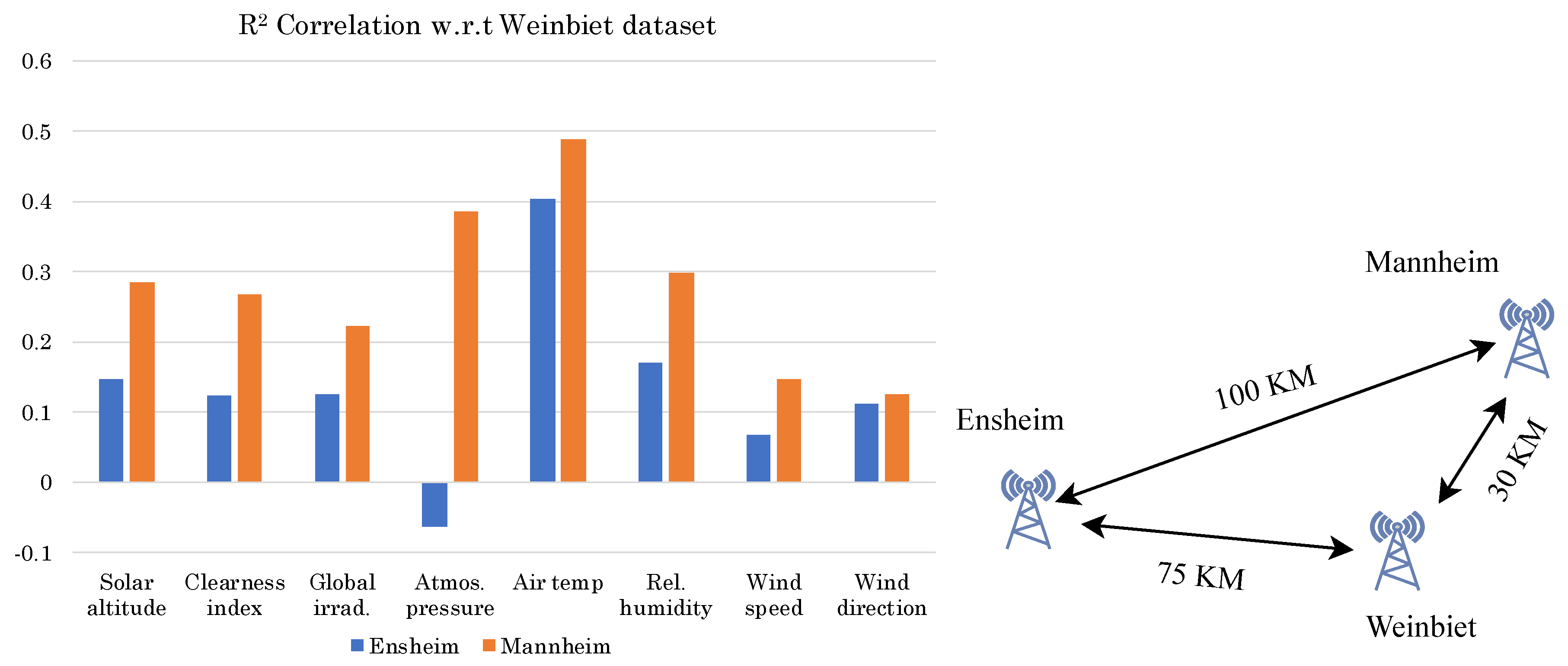
A third climate, Weinbiet, which has measured diffuse irradiance values, is selected to test for generalizabilty. The Weinbiet weather station (as shown in Figure 2) is located between Mannheim and Ensheim but is considerably closer to the Mannheim weather station (30 KM) rather than Ensheim (75 KM).

The Weinbiet dataset is preprocessed similarly to the Ensheim and Mannheim datasets. The true diffuse fraction values from the Weinbiet dataset are only used to measure the predictive performance of the models on the Weinbiet dataset.

Testing the above models on the Weinbiet data shows that the models that are trained on Mannheim showed better performance than on the Ensheim dataset, which is clearly evident from

Table 9. The performance metrics of different models trained on Mannheim and Ensheim climates. The results show the error in the prediction of diffuse horizontal irradiance (2017 data) on Weinbiet climate (unseen dataset).

Model	Models Trained on Mannheim Dataset				Models Trained on Ensheim Dataset
	nRMSE (%)	nMBE (%)	RMSE (W/m2)	MAE (W/m2)	nRMSE (%)	nMBE (%)	RMSE (W/m2)	MAE (W/m2)
NN	27.32	0.33	42.28	24.84	29.00	−7.34	44.88	28.38
XGB	27.40	3.64	42.40	26.14	30.08	−7.32	46.55	30.66
GB	27.61	3.65	42.74	26.25	30.07	−7.30	46.54	30.66
RF	27.60	4.09	42.72	26.45	30.07	−7.79	46.54	30.29
DT	29.10	4.25	45.04	27.82	30.96	−7.60	47.92	31.15
LR	34.07	5.10	52.74	37.77	34.52	−7.64	53.43	37.37
Erbs	31.47	−0.23	48.70	29.97	33.04	−8.19	51.14	32.70

. Once again NN, XGB, GB and RF showed similar nRMSE of 27% (on Mannheim) but their nMBE’s differed significantly. In this case NN showed least nMBE of just 0.33% thus faring better than other predictive models. It can also be observed that the neural network performance on its original dataset of Mannheim (see Table 7) and unseen dataset of Weinbiet are almost similar in nRMSE of 26% and 27% respectively. Though the other models generalized similarly to NN, their nMBE increased significantly on the unseen dataset, which makes their predictions less stable due to high variation. On the other hand models trained on Ensheim seems even less reliable due to high nMBE at around −7 to −8%. These results show that models trained on Mannheim are more favorable for predictions with respect to Weinbiet.

A closer look is taken into all the three datasets in order to better understand this phenomenon. Figure 2 shows the correlation of the Weinbiet dataset with the Ensheim and Mannheim datasets. The bar plots show the correlation of each input feature from Mannheim and Ensheim datasets with respect to the Weinbiet dataset. The bar plots for input features corresponding to Mannheim show better correlation when compared to that of Ensheim, which means that the Weinbiet model is more similar to the Mannheim dataset than the Ensheim dataset. This explains that models trained on Mannheim perform better than that of Ensheim.

These results suggest that a pre-trained machine learning model, provided the training dataset is chosen carefully, can make really good predictions on unseen data.

4.4. Second Study

From the first part we concluded that NN performed well among other models, but we would like to ascertain if such reliable predictions can be made on a global scale (at least on two different continents). Apart from NN, XGB is one other approach that consistently performed comparable to NN. So in this part, two approaches namely NN and XGB are used to train the models.

The training data is a consolidated data of seven U.S. climates collected from the SURFRAD network (see Table 3) from the year 2015. Both NN and XGB models are finetuned and then validated against 2016 data. To test these models, 2016 data from four European climates (France, Spain and The Netherlands) are considered (see Table 4). Due to unavailability, wind direction and wind speed are not considered, instead satellite-based diffuse fraction (from CAMS-RAD), which is available at most places in the U.S. (NSRDB) and Europe (BSRN) is considered.

Individual models with respect to each of the seven U.S. climates are also developed to compare against the main model, i.e., the model based on the consolidated data of all the seven climates. This gives us a better picture of how good or bad the combined model performs with respect to each climate individually. For instance, the nRMSE of individual models (NN) are in the range of 25 to 31%, whereas the performance of the combined model is 27% (see

Table 10. The performance metrics of NN and XGB trained on 7 U.S. climates (2015 data). The results show the error in prediction of diffuse horizontal irradiance (2016 data) on U.S. and 4 unseen datasets of European climates.

Climate	nRMSE (%)		nMBE (%)		RMSE (W/m2)		MAE (W/m2)
	NN	XGB	NN	XGB	NN	XGB	NN	XGB
U.S.	27.58	29.00	−1.39	1.34	42.68	44.88	23.41	26.99
BON	25.48	26.35	−2.03	0.48	44.06	45.55	24.69	27.32
DRA	31.72	32.54	−5.21	−1.55	37.37	38.34	20.61	23.27
FPK	28.72	30.53	−0.14	1.86	42.96	45.66	24.00	28.08
GWN	25.36	27.05	1.05	1.43	42.50	45.33	24.40	27.75
PSU	25.67	26.07	−2.49	0.22	42.63	43.31	21.85	24.12
SXF	26.46	28.22	−0.45	2.53	41.48	44.23	21.89	26.30
TBL	31.48	34.01	−1.39	3.69	46.87	50.62	26.70	32.40
CAB	23.02	23.04	0.94	−1.04	37.91	37.94	20.45	21.39
CAR	30.03	29.60	6.90	4.31	38.99	38.44	26.13	26.14
CNR	26.23	26.31	2.96	0.18	44.28	44.43	27.57	28.14
PAL	23.48	24.48	0.62	−2.25	43.07	44.91	25.88	27.72

). This confirms that the combined model appropriately represents all the underlying climates without much disparity. While comparing the performances of NN and XGB models, it can be seen that in almost all the climates once again NN models have performed better.

4.5. Test for Generalizability

Four climates in Europe (two in France, one each in The Netherlands and Spain) are selected to test the generalizability of models that are trained on U.S. data. The bottom part of Table 10 shows the performance metrics.

The performance of NN and XGB are almost similar on European climates in most of the metrics. The nRMSE of the U.S. trained model on European datasets is between 23 to 29% and on its original dataset is 27%. This performance is even better than those of individual models performed on their original datasets (25 to 31%). This shows that these models have shown very good generalizability, in fact even better than their original performance in some cases. This performance gain can be attributed to the fact that the model trained on the consolidated dataset has seen more patterns than individual datasets.

From the above results, it is shown that the right choice of training data can improve the predictive performance of these models.

A cross comparison of the predictive models from both the studies shows a more interesting result.

Table 11. Performance of all the three neural network models from both studies on the unseen dataset of Weinbiet (2017 data).

Model	nRMSE (%)	nMBE (%)	RMSE (W/m2)	MAE (W/m2)
	NN(Mannheim)	27.32	0.33	42.28	24.84
NN(Ensheim)	29.00	−7.34	44.88	28.38
NN(U.S)	29.62	8.89	45.85	26.67

shows the performance of all the three NNs on the dataset of Weinbiet. It can be observed that the model trained based on the Mannheim dataset performs better than Ensheim dataset or a combination of U.S. datasets. The nRMSE of NN (Mannheim) is 27% whereas the NN (Ensheim) and NN (U.S) achieved around 29%. Though the model trained on the consolidated dataset of U.S. climates learned more weather patterns, its performance is overshadowed by the NN (Mannheim), which was trained on local data. Since Mannheim data correlates well with Weinbiet (see Figure 2), here NN (Mannheim) has the advantage.

Neverthless the performance of NN models (Ensheim and the U.S.) does not deviate too much from that of Mannheim. Therefore, the following conclusions can be made about choosing the training data:

• When the predictions are to be done on a microclimate level with high precision, choosing a local training dataset with a good correlation to the test dataset would be a better choice.
• To make predictions for a variety of climates, a generic model trained on a combination of different climate datasets, does an excellent job.

Since the general availability of the measured data of diffuse irradiance is scarce, this approach of using a pre-trained model along with generally available data from local weather stations gives easy access to accurate diffuse irradiance data.

5. Conclusions

The main goal of this article was to test the generalization capability of the hourly diffuse horizontal irradiance prediction models and also to understand the factors that can improve their performance. The experiments in this study were divided into two parts.

In the first part, seven predictive approaches (six machine learning and one polynomial) were each trained on two German climates (Mannheim and Ensheim). They were first finetuned and validated on their respective climates before they were tested on a third German climate (Weinbiet). We observed that among all the considered approaches, neural networks and XGBoost have exhibited good generalization capabilities when compared to others. Neural networks consistently performed with low mean absolute error (MAE) of 22 W/m² on validation datasets of both the climates (Mannheim and Ensheim). While testing on a third climate (Weinbiet), it is observed that the neural network model trained on Mannheim (24 W/m²) performed better than that of Ensheim (28 W/m²). This was a bit surprising as both climates (Mannheim and Ensheim) are close to the third climate (Weinbiet). A quick look into the datasets of all three climates revealed that the Weinbeit dataset (test set) correlates better with Mannheim than Ensheim, which explains the reason behind a better performance of the model, for example, trained on the Mannheim dataset. Though the neural network performed better in all the tests at the local level (German climates), we would like to confirm if it can reliably make good predictions on a global level. Therefore, we shortlisted neural networks and the XGBoost model for our next part to test on more climates.

In the second part, the data was taken from seven different climates in the U.S. and is consolidated and then used to train neural networks and XGBoost models. These models are then tested on four European climates (two from France, one each from The Netherlands and Spain). Once again Neural networks did a great job with MAE of 23 W/m² on its validation set and generalized well on European climates with MAE in the range 20–27 W/m². Individual models for each of the U.S. climates are also developed for a comparison. These models also achieved MAE in the range of 20–26 W/m². This indicates that the developed neural networks showed their original performance even on unseen European datasets. Such generalization capability is seldom achieved but in this case it is possible because the model is trained on a consolidated training set. This contributed the model to learn varied weather patterns from seven different U.S. climates and make good predictions on European climates.

Both studies conclude that neural networks are excellent predictors and careful selection of training data can improve their performance considerably. Neural networks seem like a black box model due to the complex relationships between neurons, but they showed better predictions than their counterparts. In this regard, XGBoost fared surprisingly close to neural networks. Considering the time required to train and validate a neural network model, an XGB model did an excellent job with performance on par with neural networks.

This research has several practical applications especially for the simulation tools that need diffuse and direct components of the solar radiation. Researchers who use standard weather files in their simulations, can benefit from these trained models by incorporating directly into their tools.

References

1. Crawley, D.B.; Lawrie, L.K.; Pedersen, C.O.; Winkelmann, F.C. Energy plus: Energy simulation program. ASHRAE J. 2000, 42, 49–56. [Google Scholar]
2. Beckman, W.A.; Broman, L.; Fiksel, A.; Klein, S.A.; Lindberg, E.; Schuler, M.; Thornton, J. TRNSYS The most complete solar energy system modeling and simulation software. Renew. Energy 1994, 5, 486–488. [Google Scholar] [CrossRef]
3. Hoffmann, S.; Lee, E.S.; McNeil, A.; Fernandes, L.; Vidanovic, D.; Thanachareonkit, A. Balancing daylight, glare, and energy-efficiency goals: An evaluation of exterior coplanar shading systems using complex fenestration modeling tools. Energy Build. 2016, 112, 279–298. [Google Scholar] [CrossRef] [Green Version]
4. Ward, G.J. The RADIANCE lighting simulation and rendering system. In Proceedings of the 21st Annual Conference on Computer Graphics and Interactive Techniques, Orlando, FL, USA, 24–29 July 1994; ACM: New York, NY, USA, 1994. [Google Scholar]
5. Hoffmann, S.; McNeil, A.; Lee, E.S.; Kalyanam, R. Discomfort Glare with Complex Fenestration Systems and the Impact on Eergy Use When Using Daylighting Control; U.S. Department of Energy Office of Scientific and Technical Information: Oak Ridge, TN, USA, 2015.
6. Liu, B.Y.H.; Jordan, R.C. The interrelationship and characteristic distribution of direct, diffuse and total solar radiation. Sol. Energy 1960, 4, 1–19. [Google Scholar] [CrossRef]
7. Orgill, J.F.; Hollands, K.G.T. Correlation equation for hourly diffuse radiation on a horizontal surface. Sol. Energy 1977, 19, 357–359. [Google Scholar] [CrossRef]
8. Erbs, D.G.; Klein, S.A.; Duffie, J.A. Estimation of the diffuse radiation fraction for hourly, daily and monthly-average global radiation. Sol. Energy 1982, 28, 293–302. [Google Scholar] [CrossRef]
9. Reindl, D.T.; Beckman, W.A.; Duffie, J.A. Diffuse fraction correlations. Sol. Energy 1990, 45, 1–7. [Google Scholar] [CrossRef]
10. Boland, J.; Scott, L.; Luther, M. Modelling the diffuse fraction of global solar radiation on a horizontal surface. Environ. Off. J. Int. Environ. Soc. 2001, 12, 103–116. [Google Scholar] [CrossRef]
11. Ruiz-Arias, J.A.; Alsamamra, H.; Tovar-Pescador, J.; Pozo-Vázquez, D. Proposal of a regressive model for the hourly diffuse solar radiation under all sky conditions. Energy Convers. Manag. 2010, 51, 881–893. [Google Scholar] [CrossRef]
12. Soares, J.; Oliveira, A.P.; Božnar, M.Z.; Mlakar, P.; Escobedo, J.F.; Machado, A.J. Modeling hourly diffuse solar-radiation in the city of São Paulo using a neural-network technique. Appl. Energy 2004, 79, 201–214. [Google Scholar] [CrossRef]
13. Elminir, H.K.; Azzam, Y.A.; Younes, F.I. Prediction of hourly and daily diffuse fraction using neural network, as compared to linear regression models. Energy 2007, 32, 1513–1523. [Google Scholar] [CrossRef]
14. Ihya, B.; Mechaqrane, A.; Tadili, R.; Bargach, M. Prediction of hourly and daily diffuse solar fraction in the city of Fez (Morocco). Theor. Appl. Climatol. 2015, 120, 737–749. [Google Scholar] [CrossRef]
15. Berrizbeitia, S.E.; Jadraque Gago, E.; Muneer, T. Empirical Models for the Estimation of Solar Sky-Diffuse Radiation. A Review and Experimental Analysis. Energies 2020, 13, 701. [Google Scholar] [CrossRef] [Green Version]
16. Dervishi, S.; Mahdavi, A. Computing diffuse fraction of global horizontal solar radiation: A model comparison. Sol. Energy 2012, 86, 1796–1802. [Google Scholar] [CrossRef] [Green Version]
17. Montgomery, D.C.; Peck, E.A.; Vining, G.G. Introduction to Linear Regression Analysis; John Wiley & Sons: Hoboken, NJ, USA, 2012; Volume 821. [Google Scholar]
18. Quinlan, J.R. Simplifying decision trees. Int. J. Man Mach. Stud. 1987, 27, 221–234. [Google Scholar] [CrossRef] [Green Version]
19. Breiman, L. Random forests. Mach. Learn. 2001, 45, 5–32. [Google Scholar] [CrossRef] [Green Version]
20. Friedman, J.H. Greedy function approximation: A gradient boosting machine. Ann. Stat. 2001, 1189–1232. [Google Scholar] [CrossRef]
21. Chen, T.; Guestrin, C. Xgboost: A scalable tree boosting system. In Proceedings of the 22nd Acm sigkdd International Conference on Knowledge Discovery and Data Mining, San Francisco, CA, USA, 13–17 August 2016; ACM: New York, NY, USA, 2016. [Google Scholar]
22. Chatrchyan, S.; Hmayakyan, G.; Khachatryan, V.; Mousa, J.; Adam, W.; Bauer, T.; Bergauer, T.; Bergauer, H.; Dragicevic, M.; Erö, J. The CMS experiment at the CERN LHC. J. Instrum. 2008, 3, S08004-1. [Google Scholar]
23. Hassoun, M.H. Fundamentals of Artificial Neural Networks; MIT Press: Cambrifge, MA, USA, 1995. [Google Scholar]
24. Rumelhart, D.E.; Hinton, G.E.; Williams, R.J. Learning internal representations by error propagation. In Parallel Distributed Processing: Explorations in the Microstructure of Cognition; MIT Press: Cambridge, MA, USA, 1986; Volume 1. [Google Scholar]
25. Bergstra, J.; Bengio, Y. Random search for hyper-parameter optimization. J. Mach. Learn. Res. 2012, 13, 281–305. [Google Scholar]
26. Pedregosa, F.; Varoquaux, G.; Gramfort, A.; Michel, V.; Thirion, B.; Grisel, O.; Blondel, M.; Prettenhofer, P.; Weiss, R.; Dubourg, V.; et al. Scikit-learn: Machine Learning in Python. J. Mach. Learn. Res. 2011, 12, 2825–2830. [Google Scholar]
27. Prechelt, L. Early stopping-but when? In Neural Networks: Tricks of the Trade; Springer: Berlin/Heidelberg, Germany, 1998; pp. 55–69. [Google Scholar]
28. Hinton, G.E.; Srivastava, N.; Krizhevsky, A.; Sutskever, I.; Salakhutdinov, R.R. Improving neural networks by preventing co-adaptation of feature detectors. arXiv 2012, arXiv:1207.0580v1. [Google Scholar]
29. Srivastava, N.; Krizhevsky, A.; Sutskever, I.; Salakhutdinov, R.R. Dropout: A simple way to prevent neural networks from overfitting. J. Mach. Learn. Res. 2014, 15, 1929–1958. [Google Scholar]
30. DWD. CDC (Climate Data Center): Historical 10-Minute Station Observations for Germany. Available online: https://opendata.dwd.de (accessed on 15 June 2018).
31. Augustine, J.A.; DeLuisi, J.J.; Long, C.N. SURFRAD–A national surface radiation budget network for atmospheric research. Bull. Am. Meteorol. Soc. 2000, 81, 2341–2358. [Google Scholar] [CrossRef] [Green Version]
32. Driemel, A.; Augustine, J.; Behrens, K.; Colle, S.; Cox, C.; Cuevas-Agulló, E.; Denn, F.M.; Duprat, T.; Fukuda, M.; Grobe, H.; et al. Baseline Surface Radiation Network (BSRN): Structure and data description (1992–2017). Earth Syst. Sci. Data 2018, 10, 1491–1501. [Google Scholar] [CrossRef] [Green Version]
33. Diepenbroek, M.; Grobe, H.; Reinke, M.; Schindler, U.; Schlitzer, R.; Sieger, R.; Wefer, G. PANGAEA—An information system for environmental sciences. Comput. Geosci. 2002, 28, 1201–1210. [Google Scholar] [CrossRef] [Green Version]
34. Sengupta, M.; Xie, Y.; Lopez, A.; Habte, A.; Maclaurin, G.; Shelby, J. The national solar radiation data base (NSRDB). Renew. Sustain. Energy Rev. 2018, 89, 51–60. [Google Scholar] [CrossRef]
35. Qu, Z.; Oumbe, A.; Blanc, P.; Espinar, B.; Gesell, G.; Gschwind, B.; Klüser, L.; Lefèvre, M.; Saboret, L.; Schroedter-Homscheidt, M.; et al. Fast radiative transfer parameterisation for assessing the surface solar irradiance: The Heliosat-4 method. Meteorologische Zeitschrift 2017, 26, 33–57. [Google Scholar] [CrossRef]
36. Robbins, H.; Monro, S. A stochastic approximation method. Ann. Math. Stat. 1951, 400–407. [Google Scholar] [CrossRef]
37. Hoerl, A.E.; Kennard, R.W. Ridge regression: Biased estimation for nonorthogonal problems. Technometrics 1970, 12, 55–67. [Google Scholar] [CrossRef]
38. Chollet, F. Keras. Available online: https://keras.io/ (accessed on 18 April 2020).
39. Clevert, D.A.; Unterthiner, T.; Hochreiter, S. Fast and accurate deep network learning by exponential linear units (elus). arXiv 2015, arXiv:1511.07289. [Google Scholar]
40. Han, J.; Moraga, C. The Influence of the Sigmoid Function Parameters on the Speed of Backpropagation Learning; International Workshop on Artificial Neural Networks; Springer: Berlin/Heidelberg, Germany, 1995. [Google Scholar]
41. Kingma, D.P.; Ba, J. Adam: A method for stochastic optimization. arXiv 2014, arXiv:1412.6980v9. [Google Scholar]
42. Cover, T.M.; Thomas, J.A. Elements of Information Theory; John Wiley & Sons: Hoboken, NJ, USA, 2012. [Google Scholar]
43. Coefficient of Determination—Wikipedia. Available online: https://en.wikipedia.org/wiki/Coefficient_of_determination (accessed on 18 April 2020).
Figure 1. Mutual information and R 2 correlation coefficients of input features with respect to output F d for both datasets.
Energies 13 04868 g001
Figure 2. Comparison of the Ensheim and Mannheim datasets with respect to the Weinbiet dataset (also relative positions of weather stations).
Energies 13 04868 g002