Analysis of AMI Communication Methods in Various Field Environments


1
Department of Electronics Engineering, Hankuk University of Foreign Studies, Yongin-si, Gyeonggi-do 17035, Korea
2
Research Center for Electrical and Information Technology, Seoul National University of Science & Technology, Seoul 01811, Korea
3
Department of Electronics and Information Engineering, Hansung University, Seoul 02876, Korea
*
Author to whom correspondence should be addressed.
Energies 2020, 13(19), 5185; https://0-doi-org.brum.beds.ac.uk/10.3390/en13195185
Submission received: 31 August 2020
/
Revised: 22 September 2020
/
Accepted: 29 September 2020
/
Published: 5 October 2020
(This article belongs to the Section A1: Smart Grids and Microgrids)
Abstract
:In order to construct an efficient on-site communication network for an advanced metering infrastructure (AMI) in Korea, the high-speed power line communication (HS PLC), wireless smart utility network (Wi-SUN), and ZigBee modems are currently being used. In this paper, we first quantitatively analyze the communication performances of HS PLC, Wi-SUN, and ZigBee modems for AMI through both experimental testbeds and practical environment sites. For practical AMI sites, we selected 18 sites with 48 measurement points and classified the sites into five areas, and conducted measurements of signal and noise power spectra on the sites. We then derived linear regression models for received powers according to areas. Through the constructed models, we can efficiently choose an appropriate communication method and plan a methodology for building an AMI network depending on the area type. Furthermore, using the constructed regression models, we provided graphical simulation tools of received powers for both PLC and wireless communication methods based on a distribution information map.

1. Introduction
In order to respond to the global climate change crisis, renewable energies are spreading worldwide as energy sources [1,2]. As the sharing of renewable energy in the electric power system increases, it becomes difficult to operate the electric power system stably. As one of the ways to solve this problem, the need for a demand management system is increasing [3,4,5,6,7]. Advanced metering infrastructure (AMI) is a key element for such demand management, and is carrying out large-scale AMI deployment projects in various countries, such as the United States, Europe, and Asian countries [5,8]. AMI generally consists of a number of smart meters, data concentrators, a meter data management server, and a network management system [9,10,11,12]. Various wired and wireless communication technologies are used to construct a stable and efficient field communication network for AMI. Recently, the number of smart meters equipped with a mobile communication modem is also increasing. In order to improve AMI communication qualities and network flexibilities, a combination of wired and wireless communication methods is used [13,14,15,16,17,18,19,20]. The power line communication (PLC) is a typical method for wired communications in AMI. The PLC method can be divided into a narrowband PLC method with hundreds of kHz bandwidth and a broadband PLC method with tens of MHz bandwidth according to the frequency bandwidth used [21,22]. G3 PLC and PRIME methods [23,24] are mainly used in Europe as narrowband PLC methods for AMI configurations, while the high-speed PLC (HS PLC, ISO/IEC12139-1) and HomePlug Green PHY (HPGP) are used for broadband PLC methods in AMI configurations [25,26,27]. The wireless communication method for AMI can be divided into 2.4 GHz band methods such as WiFi or Zigbee [25,28,29] and a sub-1 GHz band method such as wireless smart utility network (Wi-SUN) [28,30,31]. LoRa [32] can be a candidate for communication techniques to construct AMI networks. However, although LoRa has a wide coverage area, it is hard for LoRa to cope with lots of smart meter nodes in a densely populated area due to its quite low rates in the order of several kbps. Therefore, currently, the LoRa approach is not considered for the AMI networks in Korea. Therefore, in the case of designing an AMI system suitable for a customer site, it is very important for the utility to select an appropriate communication method that can meet the power supply situation and AMI service requirements. Korea Electric Power Corporation (KEPCO), a leading power company in the Republic of Korea, is pursuing a project to supply AMI systems for 22.5 million low-voltage customers from 2010 to 2020. Currently, using HS PLC and HPGP of broadband PLC methods, and Wi-SUN of wireless communication methods, KEPCO has constructed AMI systems for about 10 million low-voltage customers in Korea. It is necessary to select appropriate communication methods according to the house types for low-voltage customers in order to efficiently deploy such a large-scale AMI.
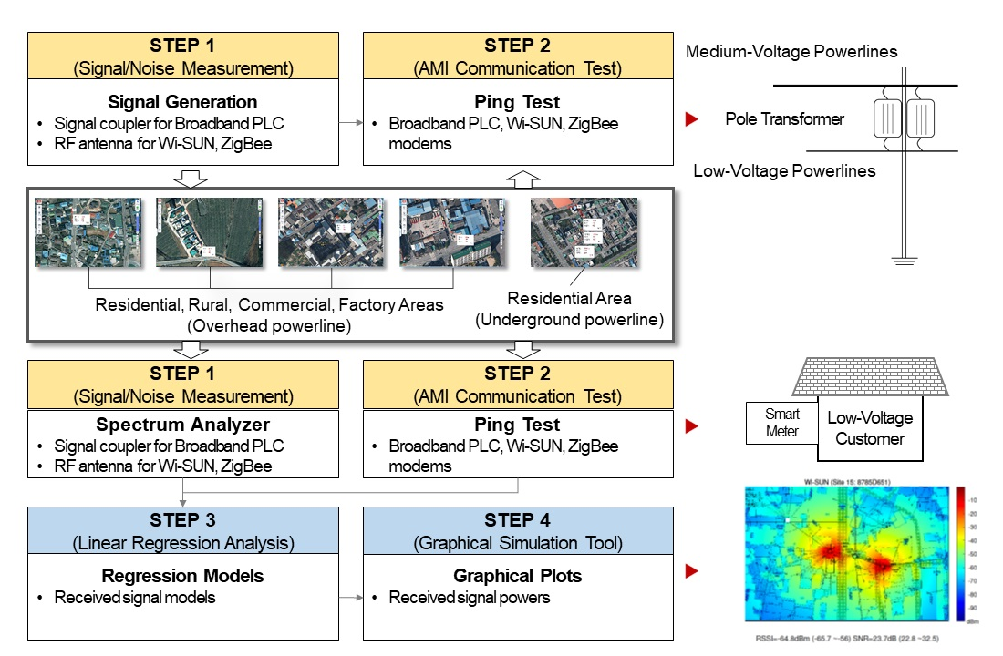
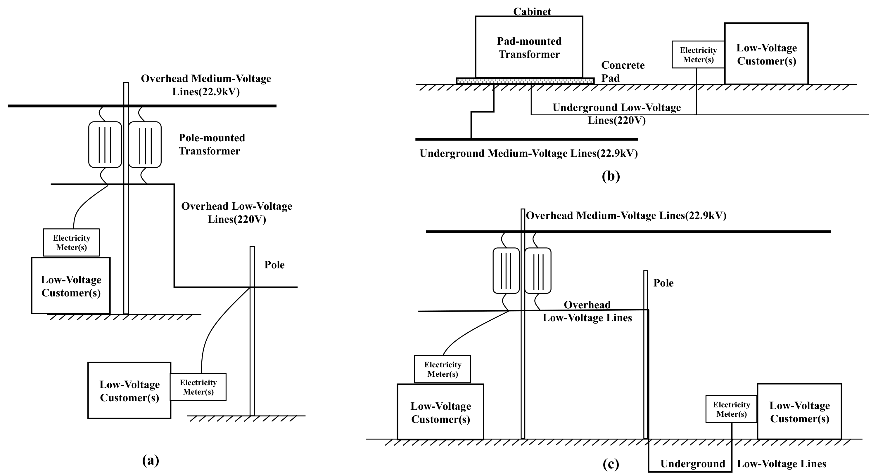
KEPCO has three methods of distribution across electric power lines for supplying electric energies to customers as shown in Figure 1. Figure 1a shows a method that supplies electric energies to the customer through overhead power lines from the pole-mounted transformer. This method has a structure that consists of electrical cables suspended by towers or poles. Even though overhead power lines have an economic advantage, they are susceptible to damage from various natural phenomena such as wind. To avoid such damages, we can transmit electrical energies through underground power lines as shown in Figure 1b even though the construction cost is relatively high. Here, the transformers are mounted on concrete pads with steel cabinets. Figure 1c is a mixed method of those from Figure 1a,b, in which from a pole-mounted transformer to poles near the customers’ electric energies are supplied through overhead power lines, and then from the poles to the customers’ electric energies are supplied through underground power lines. Figure 2 shows a configuration of the AMI system for low-voltage customers at KEPCO. An on-site AMI system is constructed around a pole-mounted or pad-mounted transformer. A data concentration unit (DCU) is installed below a pole-mounted transformer or inside a pad-mounted transformer cabinet to collect electrical data, such as the effective powers, energies, power factors, voltages, and currents, from the smart meters of customers and to set the smart meter management variables. AMI modems can be installed inside or outside near the smart meters to transmit those electrical data to DCU. The smart meter of the customer is configured in a form that one or a plurality of adjacent smart meters is clustered according to the customer structure. A low-voltage consumer modem can be built into a meter or installed as an external modem separate from the meters. Smart meters clustered within a short distance can be connected to an AMI modem through a separate wired communication method such as ISO485, so that electrical data of multiple smart meters can be collected using one modem. The types of low-voltage customers in the Republic of Korea can be characterized according to residential, rural, commercial, and factory areas. The types can also be characterized according to the wiring method that supplies electricity to the low-voltage customer as overhead and underground power lines as shown in Figure 1.
For AMI in Korea, HS PLC as a broadband PLC method, and ZigBee and Wi-SUN as wireless communication methods are currently being used. In this paper, we first experimentally measured and compared their communication performances with each other according to the types of low-voltage customers of AMI. Here, the employed broadband PLC can meet the requirements of KEPCO’s AMI communication technology in terms of high communication success rates, fast meter data reading periods of at least 15 min, time-of-use (TOU) tables, and large data transmissions such as the firmware update. However, narrowband PLC methods are excluded from the field measurement of the AMI communication method targeting low-voltage customers because these methods cannot meet the KEPCO requirements. For field environment analyses under AMI, we select practical sites according to the customer type, and measured the communication performances at each measurement point (MP), from the utility pole where the transformer is mounted, to the smart meter of the customer. Here, we use the signal and noise powers, signal-to-noise ratio (SNR), and packet error rate (PER) in evaluating the communication performances.
For the TOU billing, which requires the most frequent data transmission, the power usage data only needs to be collected within a fairly long period of 15 min. The maximum size of data transmitted by each meter is only 128 bytes. Due to these AMI operating environment characteristics, latency and channel bandwidth performances are not considered. The most important consideration for power companies to design an AMI field network is the meter reading success rate which depends on the channel packet error rate (PER), which greatly depends on the distance between the DCU and the meter. Thus, in order to efficiently assign MPs, we use New Distribution Information System (NDIS), which can graphically provide distribution information and has been used by KEPCO since 1997 for distribution planning, management, and operation. In this paper, through extensive experiments for practical AMI field environments and their regression analyses, we construct communication models for each communication method. From the constructed communication models with NDIS, we can consider an appropriate communication method and plan a methodology for constructing an AMI network based on the selected communication method.
This paper is organized in the following way. In Section 2, the employed HS PLC modem is introduced with several analysis methods. The wireless modems, which are based on Wi-SUN and ZigBee, are introduced with a linear regression analysis method in Section 3. In Section 4, practical sites of various field environments are summarized for observing the performances of the AMI communication methods. In Section 5 and Section 6, experimental results and models for the practical sites are illustrated and discussed, respectively. The conclusion is then stated in the last section.
2. Power Line Communication for AMI
In this section, we first introduce a modem that is based on HS PLC in order to examine the performance of the PLC method for practical AMI environments. We then describe measurement methods and linear regression analyses to develop communication models for various environments from the field measurements.
2.1. Power Line Communication
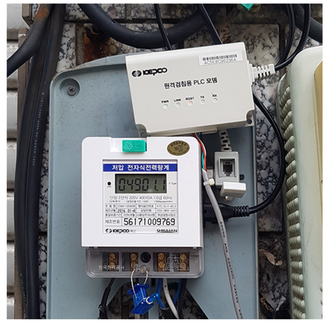
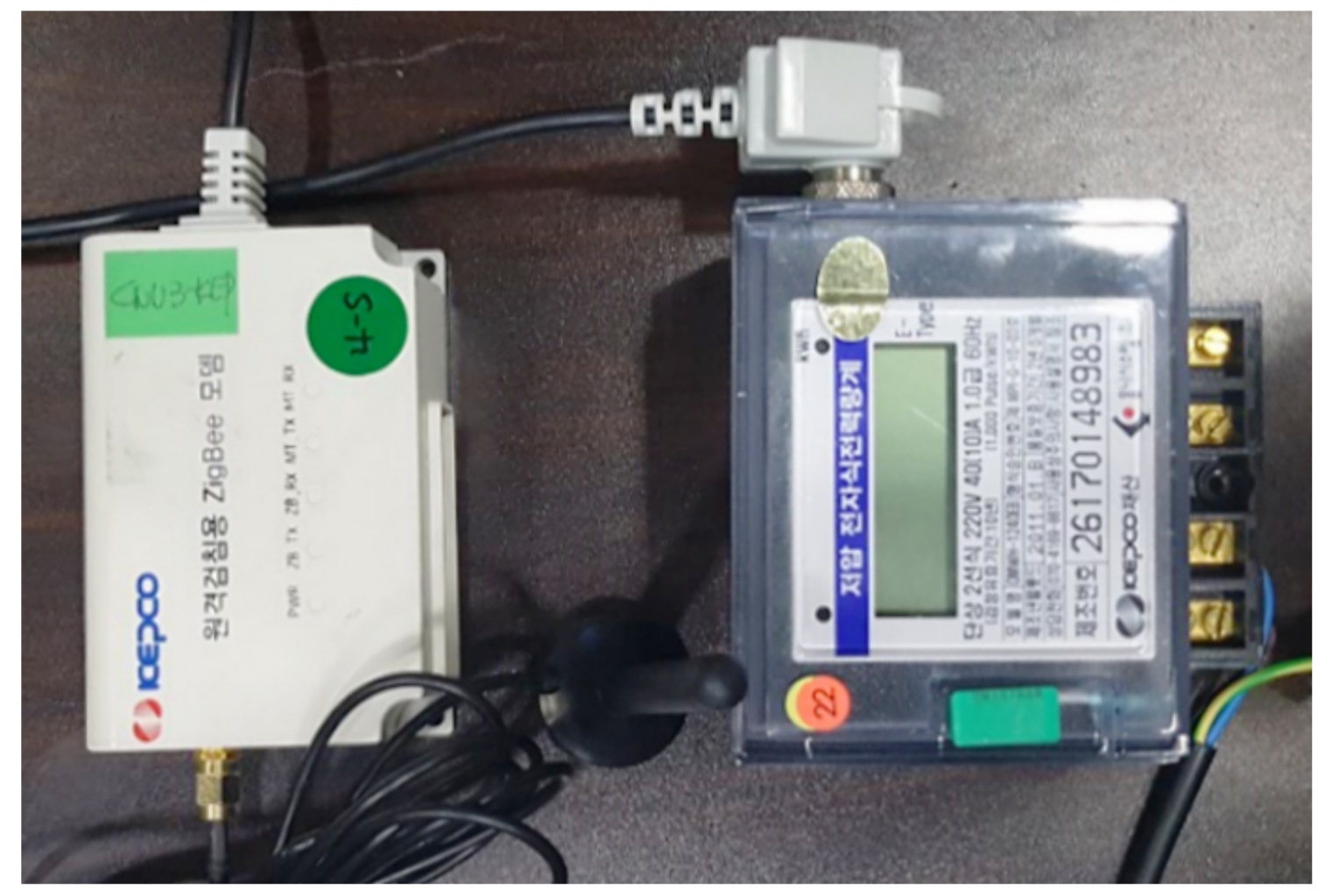
HS PLC is a broadband PLC technique developed in 2009 [25]. HS PLC uses a discrete multi-tone (DMT) for a transmission technique, which is essentially the same as the orthogonal frequency division multiplexing (OFDM). The number of the inverse Fourier transform points for OFDM is 512. There are three transmission modes: Normal, Extended Diversity (EDV), and Diversity (DV) Modes. The transmission mode can be selected according to the channel condition, information type, and the process to be performed [25]. When transmitting user data, such as metering data, Normal Mode is usually used because it has higher data rates than those of the other modes. The number of subcarriers used at Normal Mode is 152 and the subcarrier spacing is 97.66 kHz. The range of the employed frequency band is from 2.15 MHz to 23.15 MHz. For the subcarrier modulation, the differential binary phase shift keying (DBPSK), differential quadrature PSK (DQPSK), or differential 8-ary PSK (D8PSK) is used according to the tone map (TM) that is obtained from channel estimations. The rate at Normal Mode depends on the TM values and the maximum rate is 25.684 Mbps. Figure 3 shows an external type HS PLC modem connected to a smart meter (CNU Global Co. Ltd., Seongnam-si, Korea).
2.2. Measurement Methods for Power Line Communication
In order to obtain SNR values at an MP, measuring the signal and noise powers is required. The signal and noise powers can be calculated with the signal and noise spectra measured by a spectrum analyzer, respectively. A measurement block diagram of the PLC system is shown in Figure 4a. and are the frequency responses of the couplers at the transmitter and the receiver, respectively. is the frequency response of the power line. is the signal source output and is the transmitter coupler output of . The received signal through the power line is and is the output of the receiver coupler. We can notice that the spectrum of the PLC modem output is used for measurements because the PLC modem output is available only through a coupler. An example of a measured spectrum of for HS PLC is shown in Figure 4b. Here, the resolution bandwidth (RBW) is set to 10 kHz.
We first observe the frequency responses of a power line at different distances. To carry out the measurements for the observation, a low-voltage power line without power loads is deployed at a test site. The purpose of this observation is to examine the frequency response with respect to the distance. Thus, branches and loads are not connected to the power line. Two types of power lines are used for comparison: the overhead and underground power lines as shown in Figure 1. The measurements are obtained up to 200 m with 50 m intervals. The frequency responses are obtained with an RF signal generator and spectrum analyzer. A sinusoidal sweep is produced by the signal generator and this signal is provided to the power line. The magnitude spectrum of the power line is obtained by measuring the power spectrum of the received signal. The power spectrum is measured with the max-hold mode of the spectrum analyzer. We can notice that when the signal generator is used as a signal source as in Figure 4, the measured spectrum is the magnitude spectrum of through the power line and the coupler.
We now describe the frequency responses in detail. Suppose that the measurement is performed at frequency , which is given as where . Here, and are the start and end frequencies, respectively, for the spectrum analyzer span, and the number of measurement points of the spectrum analyzer is denoted as N. Let the measured power at frequency of and be denoted as and , respectively. Then the power spectral density (PSD) of x, which is denoted as , can be approximated as
where is in dBm and is the RBW of the spectrum analyzer. Let denote the total magnitude response of the power line and couplers. The magnitude response then satisfies
from the relationship of , and thus can be obtained from (2).
If the output power of the signal generator is 0 dBm at each frequency, then holds from (2). Figure 5 shows measurement results at various distances for two types of the power lines for 0 dBm. The measurement is carried out at distances of 0 to 200 m with 50-m intervals. The x-axis (horizontal axis on the left) represents the distance between the transmitter and receiver. The y-axis (horizontal axis on the right) represents the frequency in the range of 2.13 MHz to 23.156 MHz. The z-axis (vertical axis) shows the magnitude response of the channel in dB. From the results, it is clear that the attenuation increases as the distance or frequency increases. An interesting observation from Figure 5 is that the loss of the underground power line is larger than that of the overhead power line at the same distance.
The power of the PLC signal at a receiving end can be measured by the spectrum analyzer. When measuring the received power, a measurement using the PLC modem signal can be inappropriate due to the large background noise compared to limited PLC modem powers. In other words, when the received power is not high enough, the measured value cannot accurately present the signal power due to the relatively high background noise. Thus, we indirectly observe the received power by using an RF signal generator instead of the PLC modem as follows. First, we measure the magnitude response of the channel with an RF signal generator which can output high-power sine waves. Using this method, the magnitude response of the channel can be measured from (2). However, obtaining a magnitude response is further necessary instead of because the employed PLC modem provides signals after a coupler, i.e., . This response can be obtained from a relationship of
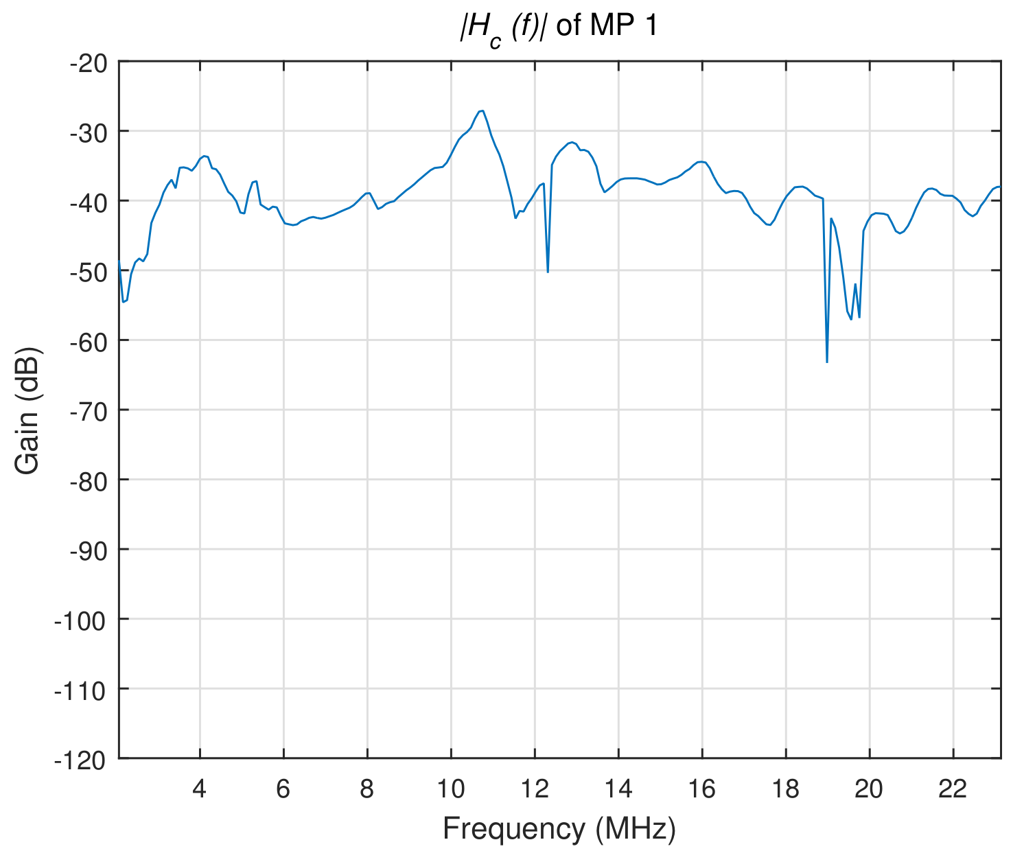
Figure 6 shows an example of , the magnitude spectrum of the power line combined with a coupler at the receiver side (MP 1 at Site 1-2, which will be described in Section 4). For the received signal , the measured power can be given as
where is the measured power of , the transmitted signal after the coupler as shown in Figure 4a. An example of the calculated power spectrum of the received signal (MP 1 at Site 1-2) is shown in Figure 7a. Let denote the total received power of signal . Then the received power can be calculated from the power spectrum as
Here, and respectively are the beginning and ending points of a significant PLC signal spectrum at the spectrum analyzer (note that ).
After removing the signal source from the power line, the background noise spectrum at the MP can then be obtained. Let denote the measured noise power at frequency with a RBW of 10 kHz. Figure 7b shows an example of a background noise spectrum obtained at MP 1 of Site 1-2. The total noise power, which is denoted as , can be calculated in a similar way of (5) as
2.3. Linear Regression Analysis for the Received Power
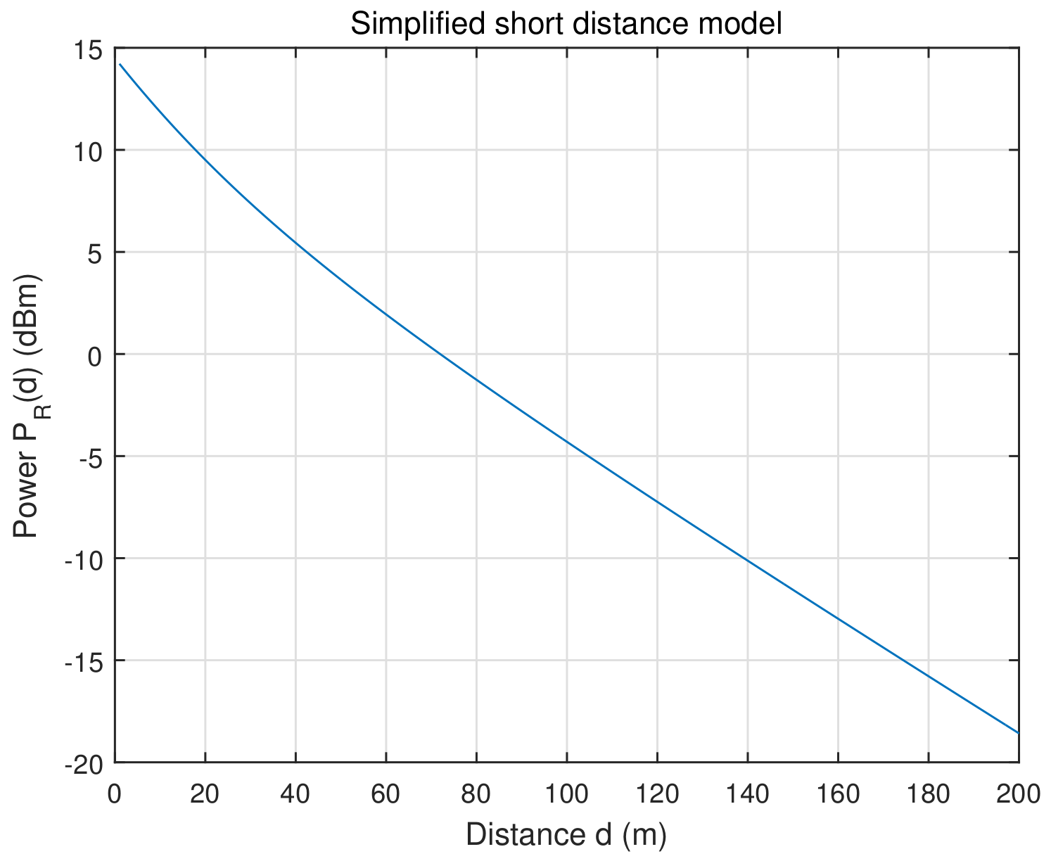
The broadband channel model in [33] describes that, when there is a single path and the length of the line is shorter than 200 m, the attenuation factor at frequency f and distance d can be simplified as
Note that the attenuation factor of (7) depends on both frequency and distance as shown in Figure 5. Let denote the power spectrum of the received PLC signal at distance d. The power spectrum can then be given as . In a similar way to (5), we can obtain , which denotes the received power with respect to the distance. Figure 8 shows an obtained curve of .
From the result of Figure 8, we can observe that the channel attenuation with respect to the path length is very close to a straight line. This result is obtained from a simplified power line model with few branches. However, for practical low-voltage power systems, a single power line may have more branches and electrical loads than the simple model case. The received power is obtained by measuring the channel response. When measuring the channel frequency response, the responses can be corrupted due to impulsive noise. Thus, the field measurement data for received PLC signal power appears in a somewhat scattered form rather than a straight line with respect to the distance.
To build a model for a relationship between the distance and the received power from the measurement results, we conduct a regression analysis [34]. The regression analysis is a statistical method to examine the relationship between two or more variables. In this paper, we use the linear regression analysis because the theoretical relationship between the distance and the received power is close to an affine function. Here, from a linear regression model, the received power can be expressed as follows.
where (dBm/m) and (dBm) are regression coefficients. Here, we call and the attenuation rate (AR) and the received power at 0 m, respectively. We find the coefficients and by minimizing a mean squared error between the measurements and the corresponding values on the straight line. Thus, the equation obtained by a linear regression analysis gives an optimal straight line in the sense of minimum mean squared error for a PLC model.
3. Wireless Communications for AMI
In this section, we use two types of modems, Wi-SUN and ZigBee modems, in order to test wireless communication methods for AMI. We then introduce measurement methods and a linear regression analysis to examine various field environments.
3.1. Wireless Communication Methods
Wi-SUN, which is the physical layer of IEEE 802.15.4 g, and ZigBee protocol, which is based on IEEE 802.15.4-2003, can be used as wireless communication methods for AMI applications. Before conducting experiments for practical field environments, we first evaluate the performance of wireless modems in a laboratory and line of sight (LOS) environments.
For Wi-SUN, we use two types of modems as shown in Figure 9. Wi-SUN Modem 1 (Nuritelecom Co. Ltd., Seoul, Korea) of Figure 9a contains CC1200 RFIC and CC1190 front-end IC of Texas Instruments. This modem is currently used to collect data from smart meters of AMI. Wi-SUN Modem 2 (Automan Co. Ltd., Gunpo-si, Korea) of Figure 9b contains Si4463 RFIC of Silicon Labs and SE2435L front-end IC of Skyworks. This modem can be used for more specific experiments by constructing a Wi-SUN test system as shown in Figure 10. Both modems can transmit RF signals of output powers from 25 mW (14 dBm) to 200 mW (23 dBm) by setting registers in firmware programs. Wi-SUN Modem 2 can select using an external LNA (low-noise amplifier) to increase the receiver sensitivity gain up to 16 dB. However, for practical field environment experiments, this external LNA is not used. Features of the employed Wi-SUN modems are summarized as follows.
- Transmitter and receiver frequency band: 920.5–923.5 MHz
- Channels and their spacing: 14 channels of 200 kHz
- Receiver bandwidth: 100 kHz (can be changed)
- Data transmission rate and packet size: 50 kbps at 128 bytes
- Receiver sensitivity: <−107 dBm at PER < 10% without external LNA
- Transmitter power: 25–200 mW (14–23 dBm)
The receiver sensitivity can be evaluated by connecting a fixed attenuator (8493B, −20 dB) and two-step attenuators (8494B; −11 dB with 1 dB step and 8496B; −110 dB with 10 dB step) as shown in Figure 10a. The transmitter power of the modem can be calibrated by using a spectrum analyzer or a power meter through a fixed attenuator (8493B, −20 dB) as shown in Figure 10b. For field environment experiments, the received power as well as transmitter power should be calibrated by using appropriate test systems as shown in Figure 10. A wireless modem, which is based on 2.4 GHz-ZigBee protocol, is also considered for the AMI communication. The employed ZigBee modem (CNU Global Co. Ltd.) is shown in Figure 11 and also currently used to collect data from smart meters of AMI. The right module of Figure 11 is a smart meter for low voltages and the left module is a ZigBee modem for transmitting the measured electrical energy.
3.2. Measurements for the Wireless Communication
In order to conduct wireless communications, we use a quarter-wave monopole antenna (Linx Technologies Inc., Merlin, OR, USA, ANT-916-CW-HWR-SMA) with 5 cm × 6 cm-ground plane for both master and slave modems, in which the antenna gain is 1.5 dBi. Here, the antenna unit is connected to the modem with SMA and N-type connectors through a 50 Ohm coaxial cable. Among the Wi-SUN channels, Channel 1, in which the center frequency is 920.7 MHz, and the transmitter power of 23 dBm are used to analyze the communication performance according to the following quantitative measurements:
- Package error rate (PER): 1000 MAC ping test with the package length of 128 bytes
- Received power in dBm from Receiver Signal Strength Indication (RSSI)
Both PER and received power through RSSI can be measured in Wi-SUN and ZigBee modems for practical field environments. We can also use a spectrum analyzer to precisely measure the received powers to examine a basic property of the wireless communications.
For wireless communications, because the PER curve usually shows a rapidly increasing characteristic when it reaches communication distance limits, it is difficult to identify the status of communications before the distance limits. Hence, rather than the PER values, the received powers are further useful in quantitatively observing the communication characteristics of field environments.
Here, the received power, which is denoted as p, can be theoretically given as [35]
where d is the distance between modems and f is the carrier frequency in MHz. In (9), the constant implies the antenna gain in dBi and is the transmitter power in dBm. To receive data at the receiver part, the received power p should be greater than the receiver sensitivity. For safe communication, the link budget between the received power and the receiver sensitivity should be large enough. Considering signal fluctuations due to field environments, the fade margin is from 10 dB to 25 dB.
For the Wi-SUN modems, the antenna gain is 1.5 dBi for the employed quarter-wave monopole antenna and the transmitter power is 23 dBm. Hence, the received power of (9) can be rewritten as −, for the Wi-SUN case. For example, the received power at a distance of m without obstacles was approximately −25.7 dBm. For practical applications for AMI purposes, a chip-type antenna (Linx Technologies Inc., AEK-916-CHP-ND) can be used. Even though the antenna gain of this chip antenna is 0.5 dBi, practical measurements of the attenuations at a 10 m distance yielded a difference of 5 dB. Hence, when we employ the chip antenna, we should consider a 5 dB compensation. For the ZigBee modem, we use a center frequency of 2.48 GHz and also conduct 1000 MAC ping tests with the package length of 128 bytes to measure the PER performance. We can also use RSSI values to measure the received powers. At GHz, the received power of (9) can be rewritten as − with a monopole antenna of gain 2.2 dBi (Linx Technologies Inc., ANT-DB1-RAF-SMA). At a distance of m, the received power was −32.8 dBm, which is less than that of Wi-SUN by 7.1 dB. Hence, even though the antenna gain for the ZigBee modem is better than the Wi-SUN case, the overall communication performance of the ZigBee modem can be worse than the Wi-SUN case. From (9), we can notice that the slope of p with respect to the distance of is −20. This slope can be obtained when there are no obstacles and the heights of the antenna modules of both modems are high enough. However, for practical environments, this slope will be less than the theoretical −20.
3.3. Regression Analysis for RSSI
As observed in the RSSI curve of (9), the theoretical slope is −20 under an ideal condition. However, depending on environmental conditions, this slope will be lower than −20. In a linear regression analysis [34] of this section, we will observe this practical slope. We now consider a linear model for a received power y as
where is the distance in a logarithmic scale and the constant is the received power when m, i.e., . For an ideal environmental condition, the coefficient a, which represents an AR for wireless communications, will be close to −20 as expected from (9). Using measured data of for practical field environments, we conduct a linear regression analysis based on the model of (10). We can then examine this coefficient a to evaluate the target environment. We can notice that an a much lower than −20 implies a bad environment for AMI wireless communications. From (9), the constants are respectively −25.7 dBm and −32.8 dBm for the Wi-SUN and ZigBee cases. However, for practical experiments, the measured RSSI values at the distance of m were −32 dBm and −39 dBm, respectively. These measured constants were used for the regression model of (10). Hence, using the obtained regression models of (10) for practical field environments, we can characterize a wireless communication condition of each field environment.
Hence, using the obtained regression models of (10) for practical field environments, we can characterize a wireless communication condition of each field environment.
As observed in the LOS experiments of Figure 12, from the beginning of the distance, the AR value a from the linear regression analysis is close to −20 (‘Wi-SUN modem high’ in Figure 12a). However, as the distance increases, the AR decreases to −31.0 (Figure 12b). In the LOS experiments of Figure 12a, ‘high’ implies that the antenna position is 1 m high from the ground and ‘low’ implies that the antenna position is right on the ground. In the experiment of this distance range, an RF signal generator and spectrum analyzer were also used to observe attenuations of the signal power. In Figure 13, PER experiments for the Wi-SUN modems are illustrated. In Figure 13a, we can observe the receiver sensitivities. At a reference PER of 10%, Wi-SUN modem 2 has a sensitivity of −110 dBm, which is better than that of Wi-SUN modem 1 by 3 dB. For the LOS experiment of Figure 12b, the PER results are illustrated in Figure 13b. Above the distance of 600 m, the PER curve of Wi-SUN modem 1 rapidly increases and thus a distance range around this distance can be a communication distance limit. Based on practically measured data for various field environments, this communication limit can be quantitatively observed by defining an equal-power distance (EPD) as follows.
Using the RSSI curve and a measured baseline noise for the selected channel, we can estimate a minimal communication limit as follows. Letting denote the baseline noise level in dBm for a given bandwidth, let us find the distance that satisfies an equal power as . The equal-power distance (EPD), which is denoted as , is then defined as
When we evaluate the field environment of a site, we can use this EPD . For the LOS experiment of Figure 12b, the baseline noise from the maximum function of the spectrum analyzer shows − dBm at the RBW of 100 Hz and thus the EPD is given as m. If we use the average function to acquire a baseline noise, then the baseline noise is given as − dBm at RBW of 100 Hz and the EPD value is now extended to m. For practical measurements, the communication distance was approximately 600–1000 m as observed in the PER experiment of Figure 13b. Thus, the EPD from both and can provide useful ranges on the communication distances.
4. Area Types of Field Environments
In this section, in order to analyze the AMI communication performances and construct communication models for various field environments, we select 18 sites for experimental measurements and classify these sites into five areas according to their characteristics as follows:
- Overhead Residential Area
- Overhead Commercial Area
- Overhead Rural Area
- Overhead Factory Area
- Underground Area
In Figure 14, Figure 15, Figure 16, Figure 17 and Figure 18, the NDIS maps and their aerial images of the 18 sites with 48 MPs are illustrated according to their areas, respectively. Here, the first four areas belong to the overhead power line system and the last area ‘Underground Area’ is concerned with the underground power line system. Properties of the 18 sites are also summarized in Table 1. In these tables, the distance implies the wire distance to each MP and thus has meaning for the PLC connection. Overhead Residential Area consists of 20 to 30 customers within a radius of about 100 m from the corresponding transformer. On the other hand, the Overhead Rural Area has few houses in a wide range. As mentioned in Table 1, Overhead Commercial, Rural, and Factory Areas suffer from various noises generated due to neon signs, solar power plants, and motors.
For the underground power line case of Figure 18, Site 5-1 is a residential area and Site 5-2 is an area where residential and commercial facilities are mixed as summarized in Table 1. As observed in Figure 18c, Site 5-3 is an apartment complex, which consists of eight buildings with a maximum of 20 stories and a minimum of 8 stories, and has a total of 984 households (Apartments, which receive the medium voltage of 22.9 kV, directly construct and manage their power systems, which are composed of transformers, switch gears, and meters. Hence, these apartments are not covered by KEPCO’s NDIS.). In this case, the communication measurements are conducted from the first basement distribution panel of an apartment building of 18 stories to the 1st, 8th, and 17th floors. It is known that the PLC communication performance is not good for the underground power line case. For the wireless communication case, the performance is also not good because several smart meters are usually mounted inside metal housings of different floors. This mount prevents transmit electromagnetic signals.
As shown in Figure 19a, the NDIS map can graphically provide the positions of distribution lines and power facilities, such as transformers, meters, and utility poles. In the NDIS map of Figure 19a, the blue circles mean the utility poles and the green lines between the blue circles represent the low-voltage distribution lines. The green and arrowed lines that extend from the blue circles represent the lines that supply electrical energies to the customers. The circle and three inverted triangles inside the red dotted box indicate the utility pole with three single-phase transformers installed. On the NDIS map, MP means the location of the smart meter of the customer to be measured, and can be identified by using the pole number connected to the customer. Because no distance information between measurement points is provided from the graphical information of the NDIS map, the distance information for both wired and wireless communications can be obtained by using a distance measurement function provided by Naver Map for the same location as shown in Figure 19b. In order to organize the measurement data for the analysis process after measurement, the pole numbers and the customer smart meters taken in the field survey process are displayed on the aerial images as in Figure 19b.
5. Experimental Results
In this section, according to the five types of field environment areas for the 18 sites with 48 MPs in operation, we conducted measurements of the PLC and wireless communication methods under AMI communication networks.
5.1. Measurement Results of PLC and Regression Analyses
Measurement results of the signal and noise powers of the PLC method for the 48 MPs of 18 sites are first summarized. For each area type, the measurement and modeling results are given.
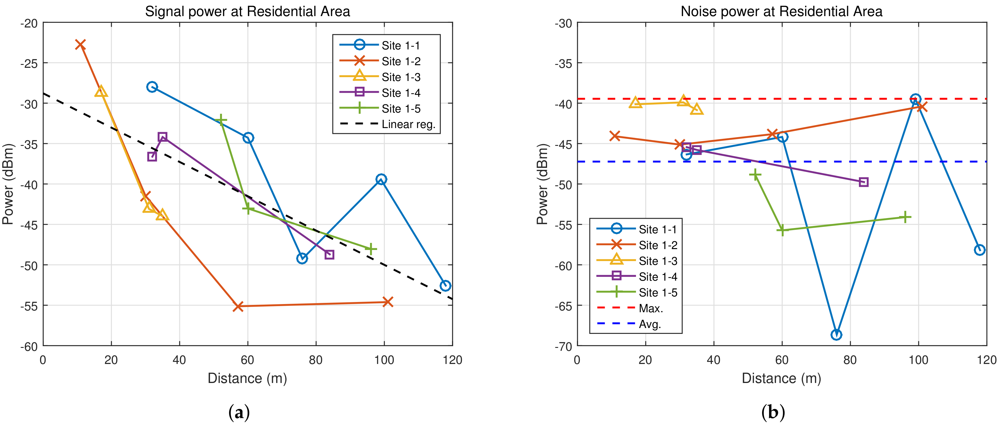
At the Overhead Residential Area, there are five sites, and each site has 3 to 5 MPs, as shown in Table 1. The received power with respect to the distance from the transmitter is shown in Figure 20a. The signal power depends on the distance and decreases as the distance increases at most of the MPs. It is observed that the slope of the received power with respect to the distance differs depending on the sites. Sites 1-2 and 1-3 have very steep slopes within a short distance range. Site 1-1 has a gentle slope between the first and second MPs. This is due to the different number of paths and/or loads connected to the power line. With the 18 MP results, a linear regression analysis was applied to make a model of the received power with respect to the distance for the Overhead Residential Area. The coefficients for the regression model in (8) were found as − and −. The model with these coefficients is shown as a black dotted line in Figure 20a. Noise spectra were also measured and stored in the average mode, and then the stored spectrum was converted to the noise power. The noise power measured in the Overhead Residential Area is shown in Figure 20b. The MPs were the same as where the signal powers were measured, and the measurements were taken at a total of 18 points. From the results, it is observed that the noise power is independent of the distance. However, the noise power depends on the environment of MP such as the area types and number of loads connected to the power line. The noise power was in a range of −68.6 dBm to −39.5 dBm. The difference between the minimum and maximum values was as large as 30 dB and thus it was difficult to estimate the noise power at a given point. Thus, two values of the noise power are used; the maximum and the average values. The maximum value is indicated by a dotted red line and the average value is indicated by a dotted blue line in Figure 20b. Here, the average value of the noise power was −47.2 dBm.
The Overhead Commercial Area consists of small shops, where many power line branches with short paths are present. Figure 21a shows the powers of received signals. The measurements were taken at 10 MPs. From the results, we can observe that the received power decreases as the distance increases at most of the MPs. We can also notice that even at the same measurement site, the ARs were not the same. At Site 2-4, the third MP had more received power than the second MP case, and even the third MP was a little farther than the second MP case. This is due to different numbers of branches at the MPs. An MP with more branches may suffer more attenuation. With the 10 MP results, a linear regression analysis was applied to model the received power with respect to the distance for the Overhead Commercial Area. The coefficients for the regression model were found as − and −. The line of the regression model is shown as a black dotted line in Figure 21a. The noise power ranged form −53.0 dBm to −33.0 dBm. The difference between the maximum and minimum was about 20 dB, which is relatively small. However, the average noise power at the Overhead Commercial Area was relatively large. The maximum value is indicated by a red dotted line and the average value (−43.2 dBm) is the blue dotted line in Figure 21b.
The Overhead Rural Area was characterized by small numbers of branches and long the path. Figure 22a shows the received powers with respect to the distance. The measurements were taken at 8 MPs. The regression coefficients for the model were found as − and −. The model with these coefficients is shown as a black dotted line in Figure 22a. The noise power ranged from −47.3 dBm to −34.0 dBm. The difference between the maximum and minimum was about 13.3 dBm, which is also relatively small. The maximum value is indicated by a red dotted line and the average value (−40.0 dBm) by the blue dotted line in Figure 22b. The average noise power at the Overhead Rural Area was rather large because of the solar-power panels at the Overhead Rural Area. Note that the solar-power panel system usually generates a lot of background noise.
The Overhead Factory Area was characterized by small numbers of branches and short path length. Figure 23a shows the received powers with respect to the distance. The measurements were made at 5 MPs. There were two MPs at Site 4-3 and they had equal path lengths at 10 m. An MP had about −24.6 dBm for the received power, while the other MP had about −37.3 dBm. In spite of the same path length, the difference of the received signal powers was about 12.7 dBm, which is a rather large value. The results at Site 4-1 show that the first MP at 10 m suffers more attenuation than the case of the second MP at 22 m. These results show somewhat different trends than those obtained in other areas. These trends will be discussed in Section 6 in more detail. With the 5 MP results, a linear regression analysis was conducted to model the received power with respect to the distance for the Overhead Factory Area. The coefficients for the model were found as − and −. The model with these values is shown as a black dotted line in Figure 23a. The noise power ranged from −49.0 dBm to −35.1 dBm. The difference between the maximum and minimum was about 13.9 dB, which is relatively small. The maximum value is indicated by a red dotted line and the average value by a blue dotted line in Figure 23b. The average noise power was −43.4 dBm, which is relatively large compared to those of other areas.
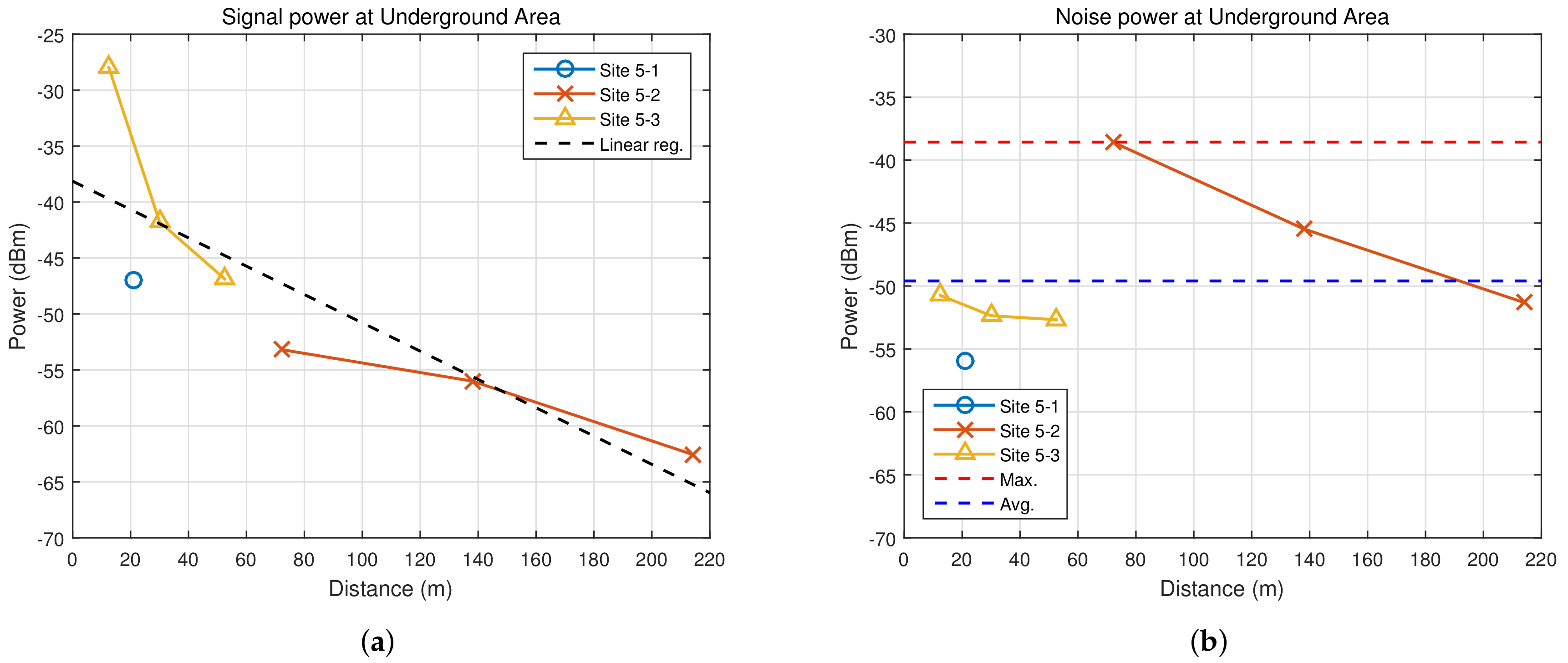
The measurements at Underground Areas were taken at 7 MPs. Figure 24a shows the received powers with respect to the distance. With the 7 MP results, a linear regression analysis was conducted and the coefficients for the model were found as - and −. The model with these values is shown as a black dotted line in Figure 24a. The noise power ranges from −56.0 dBm to −38.6 dBm. The difference between the maximum and minimum was about 17.4 dB. The maximum value is indicated by a red dotted line and the average value (−49.6 dBm) is indicated by a blue dotted line in Figure 24b.
5.2. Measurement Results of the Wireless Communications and Regression Analyses
In this section, the RSSI measurement results of the wireless communication methods for the 18 sites with 48 MPs are summarized within the five environment areas. We then conduct the linear regression analyses of (10) to construct wireless models. In the following Figure 25, Figure 26, Figure 27, Figure 28 and Figure 29, the solid lines imply measured RSSI values and the dotted lines imply measured baseline noise.
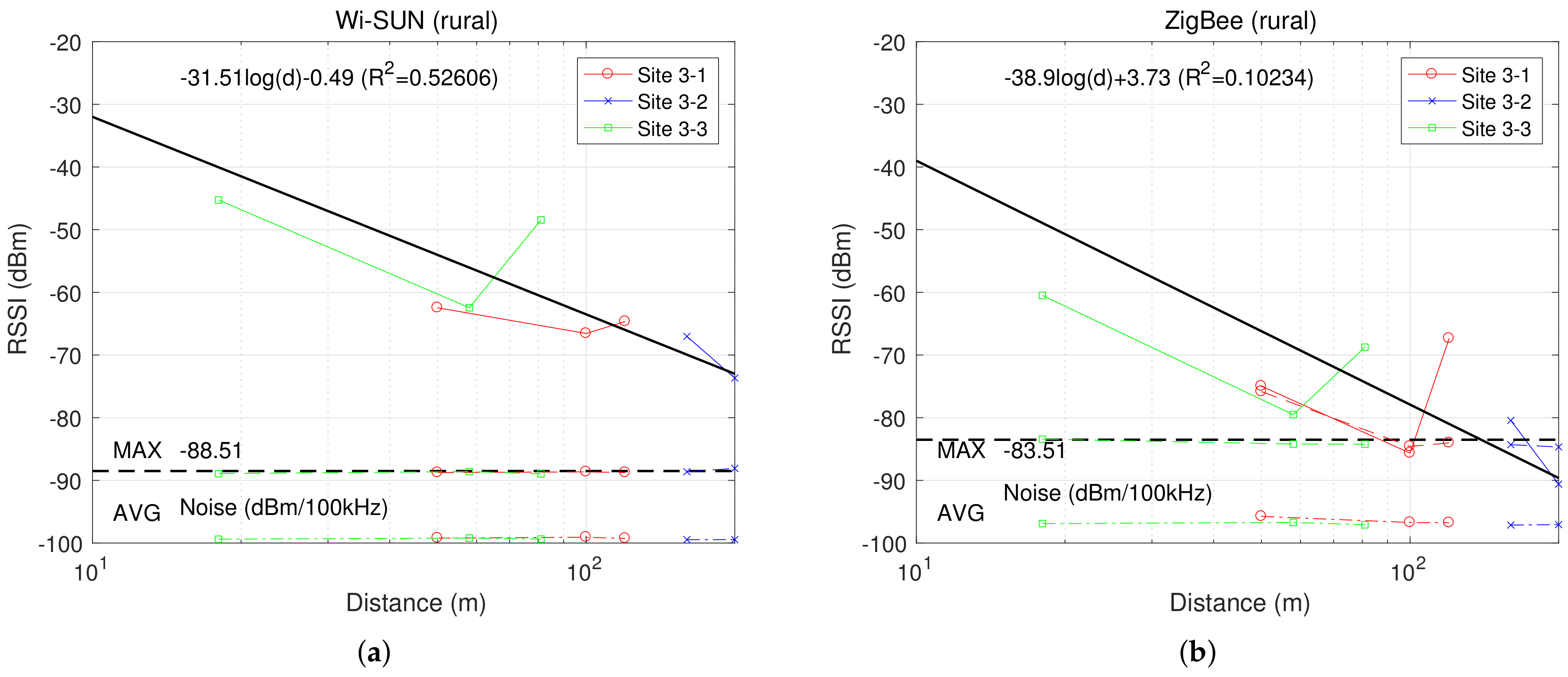
We first summarize the experiment results of the overhead power lines. For the Overhead Residential Area, the measured results are illustrated in Figure 25. Both Wi-SUN and ZigBee modems provide similar ARs of −44. However, the start point of the RSSI curve of Wi-SUN was better than the ZigBee case by 3.4 dB and the baseline noise of Wi-SUN was lower than the ZigBee case by 6.4 dB. Hence, the Wi-SUN modem had a better margin than the ZigBee case by 9.8 dB. For the Overhead Commercial Area, the measured results are illustrated in Figure 26. The Wi-SUN modem provided an AR of − and the ZigBee modem provided an AR of −, which was better than the Wi-SUN case by 1.8 dB. However, the baseline noise of ZigBee was higher than the Wi-SUN case by 7.4 dB. At Site 2-2 of the Overhead Commercial Area, we can notice a higher baseline noise compared to other sites. We can guess that this site is noisy and thus the communication distance is relatively short. For the Overhead Rural Area, the measured results are illustrated in Figure 27. The Wi-SUN modem provides an AR of −, which is higher than that of the ZigBee modem by 7.4 dB. Furthermore, the baseline noise of Wi-SUN was lower than the ZigBee case by 5.0 dB. For the Overhead Factory Area, the measured results are illustrated in Figure 28. The Wi-SUN modem provides an AR of −, which is similar to the ZigBee modem case of −. However, the baseline noise of Wi-SUN was lower than the ZigBee case by 8.2 dB.
For Underground Area, the measurement results for each MP are illustrated in Figure 29. We can notice that the communication characteristics vary greatly. Site 5-3 showed quite low RSSI values and Site 5-2 yielded RSSI values even lower than −100 dBm. On the other hand, Site 4 yielded quite good communication quality. As a result, both AR and EPD show the worst values as − and m, respectively, among the five environment areas. This observation implies that the wireless communication based on underground environments cannot provide a stable data collection for AMI. For the ZigBee case, the data collection condition was similar to the Wi-SUN case.
6. Discussions
In this section, for the PLC and wireless communications, discussions on the simulation results and constructed communication models for the classified five areas are provided.
6.1. Discussions on the Power Line Communication
Using the signal and noise powers measured in Section 5.1, SNR values at each point can be calculated after the relationship of (6). These SNR values can be used to evaluate whether a point can achieve reliable communication or not. In Table 2, coefficients for the regression models and noise powers are summarized for each area. For the received power, there is a regression curve. However, for the noise power, there are two values; one is for the average and the other is for the maximum noise powers. Therefore, two SNR curves with respect to the distance can be calculated; one is for the average SNR and the other is for the minimum SNR. The average SNR is the mean value of the SNRs at a given distance and the minimum SNR is the lowest SNR at that distance. In PLC environments, various factors, such as the number of branches, path lengths, and types of loads, can affect the SNR values. Thus, different SNR values can be observed even though the MPs have quite similar distances from the transmitters. The calculated SNR curves are illustrated in Figure 30.
Figure 30a shows the calculated SNR curves with respect to the distance at the Overhead Residential Area. The red and blue lines represent the average SNR and minimum curves, respectively. From this figure, we can estimate the average and minimum SNR values at the receiver of a given distance from the transmitter or the data concentrator unit (DCU). At all the 18 MPs of the Overhead Residential Area, the measured PER values are shown together in Figure 30a. Here, a PER value was obtained by 1000 MAC ping tests with a packet length of 128 bytes. In this PER measurement, only one-hop transmission is considered. The PER values at MPs are represented by symbol markers and the corresponding values are shown on the right vertical axis in percents. The PER values range from 0% to 100%. It is clear that higher SNR values at the receiver yield lower PER values. We can observe that the PER value shows a waterfall-like curve as the SNR value increases. In other words, if the SNR value exceeds a threshold value, then the PER value suddenly goes to 0%.
For the average SNR curve, 0 dB of SNR is obtained at 87 m. This distance is indicated as a vertical red dotted line in Figure 30a. For the MPs, which are farther than this point, the PER values are seen to be 100%. We call this region the Poor Zone for convenience. With the minimum SNR curve, 0 dB of SNR is obtained at 51 m. This distance is indicated by a vertical blue dotted line in Figure 30a. In the distance range between the blue and red dotted lines, we can notice that some MPs have no packet losses (0% PER) and the others have complete packet losses (100% PER). If an MP in this range has a good channel environment for communication, then its PER is 0%. Otherwise, it will get packet errors even up to 100%. We call this region the Gray Zone. If an MP is closer to the transmitter than the blue dotted line, then the MP can have a lower PER value. In fact, most of the MPs in this region have PER values that are close to 0%. We call this region the Good Zone. However, MPs close to the blue boundary can have large PER values even though the MPs belong to the Good Zone. At Sites 1-1, 1-2, 1-4, and 1-5, all the MPs in the Good Zone have 0% PER. The two MPs close to origin at Site 1-3 have 0% PER. However, the PER of the last MP at Site 1-3, in which the distance is 35 m, is 99% PER.
The SNR model obtained at the Overhead Commercial Area is shown in Figure 30b. At the Overhead Commercial Area, the slope of the SNR is less steep than that of the Overhead Residential Area. However, the average noise power is larger than that of the Overhead Residential Area. This is due to various noise sources, such as neon signs in stores. The average and minimum SNR values become 0 dB at the distances of 86 m and 11 m, respectively. These points are marked as vertical red and blue dotted lines, respectively. In Figure 30b, the measured results for PER are also illustrated.
The SNR model at the Overhead Rural Area is shown in Figure 30c. At this area, the SNR curve has the mildest slope among the five types of areas. This is because the power lines at the Overhead Rural Area have only a few branches. However, the average noise power is larger than those of any other types of areas. This is due to the solar power systems that the houses in rural areas have. The solar power system usually generates a lot of background noise. The 0 dB SNR value of the average and minimum SNR values occur at 120 m and 38 m, respectively. These points are marked as vertical red and blue dotted lines, respectively. The measurement results for PER at the three sites are also given in Figure 30c.
The SNR model at the Overhead Factory Area is shown in Figure 30d. The slope of this area is less steep than that of the Overhead Residential Area. The PER results are also shown in the figure. At the Overhead Factory Area, PER measurements are taken at 6 MPs. For Site 4-3, there are two MPs at the distance of 10 m and both MPs have the same 0% PER value. At the distance of 10 m, Site 4-1 also has an MP. However, the PER value at this MP is 100%. Even though they have very similar distances from the transmitters, the PER results could be quite different depending on the local noise. For the case of the Overhead Factory Area, we usually have strong inductive loads, such as powerful electrical motors. Note that these loads can cause strong background noise over several MPs and make the communication quality unpredictable.
The SNR model in the Underground Area is shown in Figure 30e. In this area, the slope of the SNR is less steep than that of the Overhead Residential Area. The received power is rather small compared to those of other areas. Moreover, the maximum noise power is quite large, resulting in a very low minimum SNR even at MPs that is close to the transmitter. The difference between the maximum and average noise powers at Underground Area is 11 dB, which is larger than the cases of the other areas and thus yields a wide Gray Zone. When preparing for the measurements in the Underground Area, it was not easy to find a point where the underground line is fully deployed from the transformer to its customers. The MP of Site 5-1 has a mixed type of Figure 1c with a 15-m overhead line and 5-m underground line as mentioned in Table 1. The overhead line is known to provide better channels for communications than the underground line case. Since the underground line is not long, the channel environment of the MP at Site 5-1 is not bad. As a result, this MP shows 0% PER. Site 5-3 is an apartment building, where the power line is inside the building not under the ground. The first MP of Site 5-3 is placed on the first floor of an apartment building and shows 0% PER. Site 5-2 has a ground transformer, which is connected to houses, stores, and a kindergarten through long underground lines. Due to the long underground path, the SNR of the received signal is very low and the PER is shown to be 100%. From these results, we can find that the communication performance of HS PLC is poor in an underground environment. We can expect that PLC modems, which are recently developed with new technologies, such as HPGP [36] and IoT PLC [37], can provide better communication performances, especially for the underground environment.
Using the regression models of Table 2 for each type of areas, the received power and SNR values are graphically simulated on the NDIS map. This visualization for the received powers and SNR values on NDIS maps is useful in planning PLC networks of AMI for a given site. When running the simulation software, we can select the starting point, which is usually a utility pole mounted with a DCU, on the NDIS map. We can then select a point where we hope to know the SNR values. The received power, minimum SNR, and average SNR obtained with the regression model can be shown. In addition, along the path, the received power can be displayed in color on the map. Figure 31 shows the visualization result on Site 1-2 as an example. The rightmost point on the map has the transmitter as a starting point and the other points on the left represent MPs. Along the path, the signal power is visualized by different colors. The SNR value corresponding to the color is displayed on the outside right of the map. For the final MP, the distance from the starting point, the received power, minimum SNR, and average SNR are displayed below the map with its corresponding zone, i.e., the Good, Gray, or Poor Zone. Figure 31a shows the simulation results at a point of 33.7 m from the starting point. The received power is −35.9 dBm, the minimum SNR is 3.57 dB, and the average SNR is 11.3 dB. Below the map, it is also displayed that the MP is in the Good Zone in terms of PER. Next, another point is tried along the line. Figure 31b shows the simulation result at a point of 102 m from the same starting point. The received power is reduced to − dBm, the minimum SNR is −10.8 dB, and the average SNR is −3.15 dB. Below the map, it is displayed that the MP is in the Poor Zone.
6.2. Discussions on the Wireless Communication
The EPD and AR results of the five environment areas are summarized in Figure 32 and Table 3. The experimental results on Wi-SUN were obtained when the transmitter power was 23 dBm (200 mW). If we decrease the transmitter power to 14 dBm (25 mW), then the EPD values will be decreased by the multiplication factor from (11). For the Overhead Residential Area as an example, the EPD value decreases to m when the transmitter power is 14 dBm. The EPD results in Table 3 are calculated using . We can observe that the EPD values of the Overhead Commercial, Rural, and Factory Areas are similar to each other as m. Especially for the Overhead Commercial Area, the EPD value is quite long, m, which is longer than that of the LOS experiment of Figure 12b, m. Hence, we can notice that the three areas have good wireless communication characteristics. However, the EPD value of the Overhead Residential Area is as low as m compared to the cases of the Overhead Commercial, Rural, and Factory areas. In other words, the Overhead Residential Area usually shows worse EPD values and hence requires more wireless nodes to secure a good communication margin. We should also note that the case of the Underground Area shows the worst communication characteristics. For this area, using PLC will provide stable communication characteristics. From the results of Figure 32 and Table 3, we can conclude that the Wi-SUN modem is usually better than the ZigBee modem for AMI communication purposes. However, for the Underground Area, in which the EPD values of the Wi-SUN and ZigBee modems are similar, we can use a 2.4 GHz communication system in a hybrid from [31].
Using the acquired regression models of (10) for each field environment area, we can graphically simulate an RF power map depending on the field environment areas. This simulation is useful in planning wireless AMI networks for a given site. From the NDIS map of the corresponding site, we can extract node locations and building structures. Considering an obstacle attenuation of 10 dB for building structures and the regression model for the corresponding field environment area, we can plot a received power map of RSSI values in dBm according to the color bar as shown in Figure 33a,b. If we place an MP at a utility pole, which is marked at an NDIS map as white rectangles as in Figure 33a, then we can obtain the received power and SNR value from the difference between the received power and the baseline noise power for the given field environment area. The site of Figure 33 belongs to the Overhead Residential Area and the obtained regression curve is − (dBm) with the maximal baseline noise of − dBm as shown in Figure 25a. For a single node example of Figure 33a, the red regions imply received powers from 10 dB to 20 dB and the received power at a location, which is indicated as a white rectangle, is −77.9 dBm. Here, the link budget is 29.1 dB if the receiver sensitivity is −107 dBm. By placing one more node as shown in Figure 33b, we can increase the link budget to 36.2 dB and enlarge the wireless coverage range. These link budgets are greater than recommended fade margins of 10 dB to 25 dB. At each position, the maximally received power can be displayed from several nodes. Hence, from the graphical simulation of Figure 33, we can determine an appropriate number of nodes and their positions in designing an AMI communication network for a given site. We can also obtain the SNR values of 10.6 dB and 23.7 dB, respectively, for Figure 33a,b. Because the SNR values of Figure 33a,b are positive, safe communications can also be expected for both cases.
6.3. Comparison of the AMI Communication Methods
In wireless communication methods, the Wi-SUN method is better than the ZigBee method in terms of the communication distance. Furthermore, the Wi-SUN method is usually better than the HS PLC method for the overhead power line case. However, for the underground power line case, the wireless communication method suffers from radio signal propagation problems due to metallic closures. Because new PLC techniques, such as HPGP and IoT PLC, can provide better communication performances than the HS PLC case [37], independent of such propagation problems, the PLC method can provide better performance compared to the wireless communication method, especially for the underground power line case. Even for the overhead power line case, the wireless communication method cannot provide a stable communication performance depending on the positions of mounted wireless antennas. Therefore, if the coverage distance is relatively short, then the HS PLC method can have an advantage over the Wi-SUN method. On the other hand, for long distances with a small number of customers, employing the wireless communication method is preferable.
7. Conclusions
In order to support future smart grid-related power services, introducing various AMI communication methods, such as wired and wireless approaches, are required. For such AMI communication approaches, generally required technical specifications, such as the frequency bandwidth and band, modulation methods, transmitter powers, and receiver sensitivities, are well-known. However, experimental analyses of actual AMI communication environments are insufficient under such specifications. In this paper, we considered the HS PLC, Wi-SUN, and ZigBee modems to quantitatively analyze the communication performances for AMI through both experimental testbeds and practical AMI sites. For practical AMI sites, we selected 18 sites with 48 MPs and classified the sites into five areas: Overhead Residential Area, Overhead Commercial Area, Overhead Rural Area, Overhead Factory Area, and Underground Area. We conducted measurements of signal and noise power spectra on 48 MPs, and derived linear regression models for received powers according to the areas. In general, the wireless communication method can provide longer communication distances for the overhead power line case. However, the performance of the wireless communication method severely deteriorates when a LOS path is not guaranteed. Thus, at the areas where a lot of obstacles between the transmitter and receiver antenna are present at high-density consumer areas such as underground power line case, PLC methods can provide better performances than wireless communication. Through the constructed models, we can efficiently choose an appropriate communication method and plan a methodology for building an AMI network. Finally, in order to visualize the communication performance of constructing AMI networks, we provided graphical simulation tools for both PLC and wireless communication methods for AMI based on NDIS. Electricity providers can utilize the results of this research to select an appropriate communication method according to the types of customers and to maintain an appropriate quality of services, such as meter reading success rate, tariff download, and power remote control.
Author Contributions
D.S.K. conducted the experiments and regression analyses in the wireless communications, and organized and refined the manuscript. B.J.C. derived the issues of evaluating the communication methods for AMI environments and managed the measurement experiments for practical AMI sites. Y.M.C. conducted the experiments and regression analyses in the power line communication. All authors have read and agreed to the published version of the manuscript.
Funding
This research was supported by grant No. C11J180034 from the Korea Electric Power Corporation (KEPCO) and Basic Science Research Program through the National Research Foundation of Korea (NRF) funded by the Ministry of Education (No. 2019R1A6A1A03032119). This research for Young Mo Chung was financially supported by Hansung University.
Acknowledgments
The experiments of this research was supported by Hyoung Joo Lee, KEPCO, Republic of Korea.
Conflicts of Interest
The authors declare no conflict of interest.
Nomenclature
| AMI | Advanced metering infrastructure |
| AR | Attenuation rate: α, α |
| DCU | Data concentration unit |
| EPD | Equal-power distance: d0 |
| MP | Measurement point |
| NDIS | New distribution information system |
| RBW | Resolution bandwidth |
| RSSI | Received signal strength indication |
| SNR | Signal-to-noise ratio |
| PER | Packet error rate |
| PLC | Power line communication |
| PSD | Power spectral density |
| Wi-SUN | Wireless smart utility network |
| BR | Resolution bandwidth |
| GA | Antenna gain in dBi |
| |H1(·)|, |H2(·)| | Magnitude responses of couplers at the transmitter and receiver |
| |Hp(·)| | Magnitude response of the power line |
| |H(·)| | Magnitude response of power line combined with couplers at the transmitter and receiver |
| |Hc(·)| | Magnitude response of the power line combined with a coupler at the receiver |
| NMAX, NAVG | Baseline noise powers with the maximum and average functions |
| PN, PS | Noise and signal power in dBm |
| PTX | Transmitter power in dBm |
| PR(d) | Received power with respect to the distance d in dBm |
| β, p10 | Received powers at 0 m and d = 10 m in dBm |
References
- IRENA. Climate Change and Renewable Energy: National Policies and the Role of Communities, Cities and Regions; (Report to the G20 Climate Sustainability Working Group); Int. Renewable Energy Agency: Abu Dhabi, UAE, 2019. [Google Scholar]
- IEA. Global Energy Review 2020; IEA: Paris, France, 2020. [Google Scholar]
- Croxton, K.; Lambert, D.; Garcia-Dastugue, S.; Rogers, D. The demand management process. Int. J. Logist. Manag. 2002, 13, 51–66. [Google Scholar] [CrossRef]
- Kim, D.S.; Son, S.Y.; Lee, J. Developments of the in-home display systems for residential energy monitoring. IEEE Trans. Consum. Electron. 2013, 59, 492–498. [Google Scholar] [CrossRef]
- Gungor, V.C.; Sahin, D.; Kocak, T.; Ergut, S.; Buccella, C.; Cecati, C.; Hancke, G.P. A survey on smart grid potential applications and communication Requirements. IEEE Trans. Ind. Inform. 2013, 9, 28–42. [Google Scholar] [CrossRef] [Green Version]
- Yu, T.; Kim, D.S.; Son, S.Y. Optimization of scheduling for home appliance in conjunction with renewable and energy storage resources. Int. Jour. Smart Home 2013, 7, 261–272. [Google Scholar]
- Bae, H.; Tsuji, T.; Oyama, T.; Uchida, K. Supply and demand balance control of power system with renewable energy integration by introducing congestion management. In Proceedings of the 2015 IEEE Eindhoven PowerTech, Eindhoven, The Netherlands, 29 June–2 July 2015; pp. 1–6. [Google Scholar]
- Popović, Ž.; Čačković, V. Advanced metering infrastructure in the context of smart grids. In Proceedings of the 2014 IEEE International Energy Conference (ENERGYCON), Cavtat, Croatia, 13–16 May 2014; pp. 1509–1514. [Google Scholar]
- US Department of Energy. Advanced Metering Infrastructure and Customer Systems: Results from the Smart Grid Investment Grant Program; DOE: Washington, DC, USA, 2016. [Google Scholar]
- George, N.; Nithin, S.; Kottayil, S.K. Hybrid key management scheme for secure AMI communications. Procedia Comput. Sci. 2016, 93, 862–869. [Google Scholar] [CrossRef] [Green Version]
- Hu, R.Q.; Qian, Y.; Zhou, J. Scalable distributed communication architectures to support advanced metering infrastructure in smart grid. IEEE Trans. Parallel Distrib. Syst. 2012, 23, 1632–1642. [Google Scholar]
- Sharma, K.; Saini, L.M. Performance analysis of smart metering for smart grid: An overview. Renew. Sustain. Energy Rev. 2015, 49, 720–735. [Google Scholar] [CrossRef]
- Ghosal, A.; Conti, M. Key management systems for smart grid advanced metering infrastructure: A survey. IEEE Commun. Surv. Tutor. 2019, 21, 2831–2848. [Google Scholar] [CrossRef] [Green Version]
- Kabalci, Y. A survey on smart metering and smart grid communication. Renew. Sustain. Energy Rev. 2016, 57, 302–318. [Google Scholar] [CrossRef]
- Zhang, J.; Hasandka, A.; Wei, J.; Alam, S.M.; Elgindy, T.; Florita, A.; Hodge, B.M. Hybrid communication architectures for distributed smart grid applications. Energies 2018, 11, 871. [Google Scholar] [CrossRef] [Green Version]
- Tavasoli, M.; Yaghmaee, M.H.; Mohajerzadeh, A.H. Optimal placement of data aggregators in smart grid on hybrid wireless and wired communication. In Proceedings of the 2016 IEEE Smart Energy Grid Engineering (SEGE), Oshawa, ON, Canada, 21–24 August 2016; pp. 332–336. [Google Scholar]
- Giustina, D.D.; Rinaldi, S. Hybrid communication network for the smart grid: Validation of a field test experience. IEEE Trans. Power Deliv. 2015, 30, 2492–2500. [Google Scholar] [CrossRef]
- Lemercier, F.; Montavont, N. Performance evaluation of a RPL hybrid objective function for the smart grid network. In Proceedings of the 17th International Conference on Ad-Hoc Networks and Wireless, Saint-Malo, France, 5–7 September 2018; pp. 27–38. [Google Scholar]
- Ghasempour, A. Optimized scalable decentralized hybrid advanced metering infrastructure for smart grid. In Proceedings of the 2015 IEEE International Conference on Smart Grid Communications (SmartGridComm), Miami, FL, USA, 2–5 November 2015; pp. 223–228. [Google Scholar]
- Barai, G.; Raahemifar, K. Optimization of distributed communication architectures in advanced metering infrastructure of smart grid. In Proceedings of the 2014 IEEE 27th Canadian Conference on Electrical and Computer Engineering (CCECE), Toronto, ON, Canada, 4–7 May 2014; pp. 1–6. [Google Scholar]
- Uribe-Pérez, N.; Angulo, I.; de la Vega, D.; Arzuaga, T.; Fernández, I.; Arrinda, A. Smart grid applications for a practical implementation of IP over narrowband power line communications. Energies 2017, 10, 1782. [Google Scholar] [CrossRef] [Green Version]
- Kim, D.S.; Chung, B.J.; Chung, Y.M. Statistical learning for service quality estimation in broadband PLC AMI. Energies 2019, 12, 684. [Google Scholar] [CrossRef] [Green Version]
- Uribe-Pérez, N.; Hernández, L.; Gómez, R.; Soria, S.; de la Vega, D.; Angulo, I.; Arzuaga, T.; Gutiérrez, L. Smart management of a distributed generation microgrid through PLC PRIME technology. In Proceedings of the 2015 International Symposium on Smart Electric Distribution Systems and Technologies (EDST), Vienna, Austria, 8–11 September 2015; pp. 374–379. [Google Scholar]
- Angulo, I.; Arrinda, A.; Fernández, I.; Uribe-Pérez, N.; Arechalde, I.; Hernández, L. A review on measurement techniques for non-intentional emissions above 2 kHz. In Proceedings of the 2016 IEEE International Energy Conference (ENERGYCON), Leuven, Belgium, 4–8 April 2016; pp. 1–5. [Google Scholar]
- ISO/IEC 12139-1. Information Technology—Telecommunications and Information Exchange between Systems—Power Line Communication (PLC) Medium Access Control (MAC) and Physical Layer (PHY)—Part 1: General Requirements; International Organization for Standardization: Geneva, Switzerland, 2009. [Google Scholar]
- Hoch, M. Comparison of PLC G3 and PRIME. In Proceedings of the 2011 IEEE International Symposium on Power Line Communications and Its Applications, Udine, Italy, 3–6 April 2011; pp. 165–169. [Google Scholar]
- Llano, A.; de la Vega, D.; Angulo, I.; Marron, L. Virtual PLC Lab enabled physical layer improvement proposals for PRIME and G3-PLC standards. Appl. Sci. 2020, 10, 1777. [Google Scholar] [CrossRef] [Green Version]
- Luan, S.; Teng, J.; Chan, S.; Hwang, L. Development of a smart power meter for AMI based on ZigBee communication. In Proceedings of the 2009 International Conference on Power Electronics and Drive Systems (PEDS), Taipei, Taiwan, 2–5 November 2009; pp. 661–665. [Google Scholar]
- Kim, D.S.; Chung, B.J.; Son, S.Y. Implementation of a low-cost energy and environment monitoring system based on a hybrid wireless sensor network. J. Sensors 2017, 2017, 5957082. [Google Scholar] [CrossRef]
- Chang, K.H.; Mason, B. The IEEE 80215.4 g standard for smart metering utility networks. In Proceedings of the 2012 IEEE Third International Conference on Smart Grid Communications (SmartGridComm), Tainan, Taiwan, 5–8 November 2012; pp. 476–480. [Google Scholar]
- Kim, A.; Han, J.; Yu, T.; Kim, D.S. Hybrid wireless sensor network for building energy management systems based on the 2.4 GHz and 400 MHz bands. Inf. Syst. 2015, 48, 320–326. [Google Scholar] [CrossRef]
- Chen, D.; Brown, J.; Khan, J.Y. 6LoWPAN based neighborhood area network for a smart grid communication infrastructure. In Proceedings of the 2013 Fifth International Conference on Ubiquitous and Future Networks (ICUFN), Da Nang, Vietnam, 2–5 July 2013; pp. 576–581. [Google Scholar]
- Zimmermann, M.; Dostert, K. A multipath model for the powerline channel. IEEE Trans. Commun. 2002, 50, 553–559. [Google Scholar] [CrossRef] [Green Version]
- Sen, A.; Srivastava, M. Regression Analysis: Theory, Methods, and Applications; Springer: New York, NY, USA, 1990. [Google Scholar]
- Stutzman, W.L.; Thiele, G.A. Antenna Theory and Design, 3rd ed.; John Wiley & Sons: New York, NY, USA, 2012. [Google Scholar]
- Alliance, H.P. HomePlug Green PHY Specification Release Version 1.1.1; HomePlug Alliance: Beaverton, OR, USA, 2013. [Google Scholar]
- Chung, Y.M. Performance comparisons of broadband power line communication technologies. Appl. Sci. 2020, 10, 3306. [Google Scholar] [CrossRef]
Figure 1.
Low-voltage distribution configurations at KEPCO, Republic of Korea. (a) Low-voltage power system using overhead power lines. (b) Low-voltage power system using underground power lines. (c) Mixed type of the overhead and underground power lines.
Figure 1.
Low-voltage distribution configurations at KEPCO, Republic of Korea. (a) Low-voltage power system using overhead power lines. (b) Low-voltage power system using underground power lines. (c) Mixed type of the overhead and underground power lines.

Figure 2.
Advanced metering infrastructure (AMI) system configuration of Korea Electric Power Corporation (KEPCO), Republic of Korea.
Figure 2.
Advanced metering infrastructure (AMI) system configuration of Korea Electric Power Corporation (KEPCO), Republic of Korea.

Figure 3.
High-speed power line communication (HS PLC) modem connected to a smart meter (CNU Global Co. Ltd.).
Figure 3.
High-speed power line communication (HS PLC) modem connected to a smart meter (CNU Global Co. Ltd.).

Figure 4.
Model of the PLC system. (a) Measurement signals for the PLC system. (b) An example of the power spectrum of the HS PLC signal at the coupler output .
Figure 4.
Model of the PLC system. (a) Measurement signals for the PLC system. (b) An example of the power spectrum of the HS PLC signal at the coupler output .

Figure 5.
Magnitude response of the PLC channel at various distances from (2). (a) Overhead power line. (b) Underground power line.
Figure 5.
Magnitude response of the PLC channel at various distances from (2). (a) Overhead power line. (b) Underground power line.

Figure 6.
Magnitude response through the power line and receiver coupler from (3).
Figure 6.
Magnitude response through the power line and receiver coupler from (3).

Figure 7.
Spectra of the received and noise signals. (a) Signal power spectrum of the received signal from (4). (b) Noise power spectrum .
Figure 7.
Spectra of the received and noise signals. (a) Signal power spectrum of the received signal from (4). (b) Noise power spectrum .

Figure 8.
Simplified short-distance model for the received power .

Figure 9.
Wi-SUN modems for the Wi-SUN measurement. (a) Wi-SUN Modem 1 (Nuritelecom Co. Ltd.). (b) Wi-SUN Modem 2 (Automan Co. Ltd.).
Figure 9.
Wi-SUN modems for the Wi-SUN measurement. (a) Wi-SUN Modem 1 (Nuritelecom Co. Ltd.). (b) Wi-SUN Modem 2 (Automan Co. Ltd.).

Figure 10.
Test system for the wireless smart utility network (Wi-SUN) measurement at line of sight (LOS) based on Wi-SUN Modem 2. (a) Measurement of the receiver sensitivity and an Receiver Signal Strength Indication (RSSI) calibration. Fixed and step attenuators (8493B, 8494B, and 8496B of Keysight) are placed between test systems that are respectively used as master and slave parts. (b) Transmitter power calibration with a spectrum analyzer.

Figure 11.
ZigBee modem for smart meters (CNU Global Co. Ltd.).

Figure 12.
LOS experiments of Wi-SUN and ZigBee modems. (a) Experiments of a range from 5 m to 200 m (Wi-SUN and ZigBee), where the attenuation rate (AR) values start from −20.0. (b) Experiments of a range from 100 m to 1000 m (Wi-SUN), where the AR value is −31.0.
Figure 12.
LOS experiments of Wi-SUN and ZigBee modems. (a) Experiments of a range from 5 m to 200 m (Wi-SUN and ZigBee), where the attenuation rate (AR) values start from −20.0. (b) Experiments of a range from 100 m to 1000 m (Wi-SUN), where the AR value is −31.0.

Figure 13.
Packet error rate (PER) test of the Wi-SUN modems. (a) Receiver sensitivity experiments. The sensitivities are <−107 dBm at PER < 10%. (b) PER test of the LOS experiment of Figure 12b.
Figure 13.
Packet error rate (PER) test of the Wi-SUN modems. (a) Receiver sensitivity experiments. The sensitivities are <−107 dBm at PER < 10%. (b) PER test of the LOS experiment of Figure 12b.

Figure 14.
New Distribution Information System (NDIS) maps for the Overhead Residential Area. (a) Site 1-1. (b) Site 1-2. (c) Site 1-3. (d) Site 1-4. (e) Site 1-5.
Figure 14.
New Distribution Information System (NDIS) maps for the Overhead Residential Area. (a) Site 1-1. (b) Site 1-2. (c) Site 1-3. (d) Site 1-4. (e) Site 1-5.

Figure 15.
NDIS maps for the Overhead Commercial Area. (a) Site 2-1. (b) Site 2-2. (c) Site 2-3. (d) Site 2-4.
Figure 15.
NDIS maps for the Overhead Commercial Area. (a) Site 2-1. (b) Site 2-2. (c) Site 2-3. (d) Site 2-4.

Figure 16.
NDIS maps for the Overhead Rural Area. (a) Site 3-1. (b) Site 3-2. (c) Site 3-3.

Figure 17.
NDIS maps for the Overhead Factory Area. (a) Site 4-1. (b) Site 4-2. (c) Site 4-3.

Figure 18.
NDIS maps for Underground Area. (a) Site 5-1. (b) Site 5-2. (c) Site 5-3.

Figure 19.
Example of the NDIS map (Site 1-2, Overhead Residential Area). (a) NDIS map with a utility pole and distribution lines. (b) Aerial photography with a utility pole and MPs.
Figure 19.
Example of the NDIS map (Site 1-2, Overhead Residential Area). (a) NDIS map with a utility pole and distribution lines. (b) Aerial photography with a utility pole and MPs.

Figure 20.
Overhead Residential Area. (a) Received power. (b) Noise power.

Figure 21.
Overhead Commercial Area. (a) Received power. (b) Noise power.

Figure 22.
Overhead Rural Area. (a) Received power. (b) Noise power.

Figure 23.
Overhead Factory Area. (a) Received power. (b) Noise power.

Figure 24.
Underground Area. (a) Received power. (b) Noise power.

Figure 25.
RSSI values for the Overhead Residential Area. (a) Wi-SUN. (b) ZigBee.

Figure 26.
RSSI values for the Overhead Commercial Area. (a) Wi-SUN. (b) ZigBee.

Figure 27.
RSSI values for the Overhead Rural Area. (a) Wi-SUN. (b) ZigBee.

Figure 28.
RSSI values for the Overhead Factory Area. (a) Wi-SUN. (b) ZigBee.

Figure 29.
RSSI values for the Underground Area. (a) Wi-SUN modem. (b) ZigBee.

Figure 30.
Signal-to-noise ratio (SNR) and PER with respect to the distance. (a) Overhead Residential Area. (b) Overhead Commercial Area. (c) Overhead Rural Area. (d) Overhead Factory Area. (e) Underground Area.
Figure 30.
Signal-to-noise ratio (SNR) and PER with respect to the distance. (a) Overhead Residential Area. (b) Overhead Commercial Area. (c) Overhead Rural Area. (d) Overhead Factory Area. (e) Underground Area.

Figure 31.
Graphical simulation of the received power for the HS PLC modem (Site 1-2, Overhead Residential Area). (a) MP at distance 33.5 m. (b) MP at distance 102 m.
Figure 31.
Graphical simulation of the received power for the HS PLC modem (Site 1-2, Overhead Residential Area). (a) MP at distance 33.5 m. (b) MP at distance 102 m.

Figure 32.
AR with respect to the equal-power distance (EPD) for the five environment areas. The Wi-SUN modem of 920 MHz provides better communication distances for all areas compared to the ZigBee case of 2.4 GHz.
Figure 32.
AR with respect to the equal-power distance (EPD) for the five environment areas. The Wi-SUN modem of 920 MHz provides better communication distances for all areas compared to the ZigBee case of 2.4 GHz.

Figure 33.
Graphical simulation of the received power for the 920 MHz Wi-SUN modems (Site 1-2, Overhead Residential Area). (a) Power map with one node, in which data concentration unit (DCU) and wireless modem are attached below the transformer. (b) Power map with two nodes, in which the wireless modem of the second node acts as a repeater.


Table 1.
Summary of the 18 Sites with 48 measurement points (MPs) in Figure 14, Figure 15, Figure 16, Figure 17 and Figure 18.
| Population | Distances | |||
|---|---|---|---|---|
| Site | Density | MPs | (Meters) | Characteristics |
| 1-1 | Middle | 5 | 32, 76, 118, 99, 60 | Small houses from 1 to 3 stories |
| 1-2 | Middle | 4 | 11, 30, 57, 101 | Small 1-story houses |
| 1-3 | 3 | 17, 31, 35 | ||
| 1-4 | Low | 3 | 35, 32, 84 | |
| 1-5 | Middle | 3 | 52, 60, 96 | |
| 2-1 | High | 2 | 6, 61 | Medium-sized commercial buildings below 10 stories |
| Noise from neon signs for PLC | ||||
| 2-2 | High | 3 | 16, 55, 72 | Medium-sized business hotels below 10 stories |
| 2-3 | High | 2 | 5, 44 | Small-sized commercial buildings less than 3 stories |
| 2-4 | Middle | 3 | 3, 44, 45 | |
| 3-1 | Low | 3 | 64, 98, 147 | Small 1-story houses |
| PV panels around the low-voltage distribution lines | ||||
| Switching noise for PLC during solar power generation | ||||
| 3-2 | Low | 2 | 140, 179 | Few houses |
| Long distances from the transformers | ||||
| 3-3 | Low | 3 | 6, 55, 90 | Small and medium-sized houses |
| Roof-type solar power plants with PV panels of kW | ||||
| 4-1 | Low | 2 | 10, 22 | Small factories below 2 stories |
| 4-2 | 1 | 49 | Short distances between customers and transformers | |
| 4-3 | 2 | 10, 10 | High-frequency noise for PLC from motors | |
| 5-1 | Middle | 1 | 21 | Multi-family houses with 3 to 4 stories |
| From the transformer to the 1st pole; overhead lines | ||||
| From the 1st pole to customers; underground lines | ||||
| 5-2 | High | 3 | 72, 138, 214 | 5-story multi-family houses and commercial buildings |
| Long-range underground low-voltage distribution lines | ||||
| 5-3 | High | 3 | 1st, 8th, 17th floors | Apartment complex of 8 buildings below 20 stories |
| from the 1st floor | Measured in the 18-story building (144 households) |
Table 2.
Summary of the regression model coefficients for PLC signal and noise powers at various areas.
Table 2.
Summary of the regression model coefficients for PLC signal and noise powers at various areas.
| Residental | Commercial | Rural | Factory | Underground | |
|---|---|---|---|---|---|
| (dBm/m) | −0.212 | −0.135 | −0.074 | −0.145 | −0.127 |
| (dBm) | −28.8 | −31.6 | −31.2 | −28.3 | −38.1 |
| Average noise power (dBm) | −47.2 | −43.2 | −40.0 | −43.4 | −49.6 |
| Maximum noise power (dBm) | −39.5 | −33.0 | −34.0 | −35.1 | −38.6 |
Table 3.
EPD and the AR for the wireless communications.
| Wi-SUN | ZigBee | |||||
|---|---|---|---|---|---|---|
| Environment Area | EPD (14 dBm) | EPD (23 dBm) | AR | EPD | AR | |
| (Meters) | a (dB/) | (Meters) | a (dB/) | |||
| Overhead | Residential | 118 | 188 | −44.4 | 94.8 | −44.1 |
| Commercial | 463 | 978 | −27.7 | 371 | −25.9 | |
| Rural | 322 | 621 | −31.5 | 139 | −38.9 | |
| Factory | 349 | 685 | −30.7 | 217 | −30.8 | |
| Underground | 31.8 | 39.6 | −93.9 | 37.0 | −79.4 | |
© 2020 by the authors. Licensee MDPI, Basel, Switzerland. This article is an open access article distributed under the terms and conditions of the Creative Commons Attribution (CC BY) license (http://creativecommons.org/licenses/by/4.0/).
Share and Cite
MDPI and ACS Style
Kim, D.S.; Chung, B.J.; Chung, Y.M. Analysis of AMI Communication Methods in Various Field Environments. Energies 2020, 13, 5185. https://0-doi-org.brum.beds.ac.uk/10.3390/en13195185
AMA Style
Kim DS, Chung BJ, Chung YM. Analysis of AMI Communication Methods in Various Field Environments. Energies. 2020; 13(19):5185. https://0-doi-org.brum.beds.ac.uk/10.3390/en13195185
Chicago/Turabian StyleKim, Dong Sik, Beom Jin Chung, and Young Mo Chung. 2020. "Analysis of AMI Communication Methods in Various Field Environments" Energies 13, no. 19: 5185. https://0-doi-org.brum.beds.ac.uk/10.3390/en13195185
Note that from the first issue of 2016, this journal uses article numbers instead of page numbers. See further details here.