Economic Impacts of the Demand Response of Electric Vehicles Considering Battery Degradation

Energy System Integration Social Cooperation Program, Institute of Industrial Science, University of Tokyo, Tokyo 113-8654, Japan
*
Author to whom correspondence should be addressed.
Energies 2020, 13(21), 5771; https://0-doi-org.brum.beds.ac.uk/10.3390/en13215771
Submission received: 5 October 2020
/
Revised: 3 November 2020
/
Accepted: 3 November 2020
/
Published: 4 November 2020
(This article belongs to the Special Issue Bidirectional Energy Transfer Technologies for Vehicle-to-Grid and Other Vehicle-to-X Applications, and Solutions to Issues Caused by High Electric Vehicle Penetration Rates)
Abstract
:The increase in the number of electric vehicles (EVs) has led to increased global expectations that the application of this technology may result in the reduction of CO2 emissions through the replacement of conventional petrol vehicles and ensure the flexibility of power systems such as batteries. In this paper, we propose a residential demand response (DR) evaluation model that considers the degradation mechanism of the EV battery and examines the effective battery operation. We adopted the already-proposed NiMnCo battery degradation model to develop an EV DR evaluation model. In this model, the battery operation is optimized to minimize the electricity and degradation costs affected by ambient temperature, battery state of charge (SOC), and depth of discharge. In this study, we evaluated the impact of the relevant parameters on the economics of the DR of EV batteries for 10 all-electric detached houses with photovoltaic system assuming multiple EV driving patterns and battery (dis)charging constraints. The results indicated that the degradation costs are greatly affected by the SOC condition. If a low SOC can be managed with a DR strategy, the total cost can be reduced. This is because the sum of the reduction of purchased cost from the utility and calendar degradation costs are higher than the increase of the cycle degradation cost. In addition, an analysis was conducted considering different driving patterns. The results showed that the cost reduction was highest when a driving pattern was employed in which the mileage was low and the staying at home time was large. When degradation costs are included, the value of optimized charging and discharging operations is more apparent than when degradation costs are not considered.
1. Introduction
The deployment of electric vehicles (EVs) has been growing rapidly in the past 10 years, resulting in a high global stock of electric passenger cars in 2018 (over 5 million). Furthermore, the International Energy Agency (IEA) predicts that this global stock will reach 250 million vehicles by 2030 based on the EV30@30 scenario [1]. The mass introduction of EVs has led to global expectations because CO2 emissions may be reduced by replacing conventional petrol vehicles and the flexibility of power systems as batteries may be ensured. Photovoltaic (PV) and wind power generation, which are predicted to increase in the future, have downsides because of the fluctuating power generation output that is dependent on the weather and time of day. Therefore, it is essential to secure flexible resources of the power system in order to stabilize the output. Flexible resources that contribute to grid stability include thermal power plant backups, renewable energy generation output control, and use of demand response (DR) at the demand side. DR refers to the control of energy storage devices on the demand side, such as the batteries of EVs and heat pump (HP) water heaters, and methods of cost-effectively utilizing these resources are being explored worldwide.
The smart charging and discharging of EV batteries, combined with the increasing number of distributed renewable energy resources, will prevent shortages in distribution capacity and contribute to the maintenance of power supply and demand. Various EV integration management models have been proposed to quantitatively evaluate the effect of EVs on the power grid. The authors have proposed a macro-model to assess the impact of EVs on DR, which integrates supply and demand to minimize the total cost of the power system using a quantitative evaluation [2]. Furthermore, a residential model has also been proposed, which aims to minimize the cost of electricity for an entire household, including EVs [3]. However, additional charge/discharge cycles of an EV, caused by DR, which shortens the battery life, were not considered in the model. As a result, the prediction of the economic impact on EV users based on a model that considers a degradation mechanism due to charge/discharge cycles is first required.
In this paper, we propose a DR evaluation model that includes the degradation mechanism of the EV battery. With this model, we also investigate the most effective battery operation. The novelty of this study is that the additional costs of calendar and cycle degradation are explicitly modeled and incorporated into an EV charge/discharge planning and operation model that can take into account the uncertainty of EV driving, which enables the comprehensive economic evaluation of DR by EVs.
The rest of this paper is organized as follows. In Section 2, the literature related to our study is reviewed. In Section 3, the battery degradation model is described. In Section 4, the EV DR evaluation model considering battery degradation is discussed. In Section 5, we present the simulation case and its results. Finally, topics for future research are presented in Section 6.
2. Literature Review
In this section, the following topics, which were significant for this research, were reviewed: (1) modeling of the degradation of the battery structure, and (2) DR evaluation of vehicle-to-grid (V2G) considering battery degradation. Thompson et al. [4] conducted a literature review on the economic effects of the degradation of lithium-ion batteries for V2G services, resulting in studies on the mechanisms of degradation, characteristics of each battery type, and examples of economic evaluations.
2.1. Modeling the Degradation of Batteries
The battery state of health (SOH) is defined by the capacity reduction (i.e., capacity fade) and the decrease in the battery output due to increased internal impedance of the battery (i.e., power fade), with the former being the most commonly discussed [4]. These degradation mechanisms result in calendar aging and cycling aging, which are aging behaviors that occur when the battery is at rest and when it is being used, respectively, and which are exacerbated by degradation drivers. Furthermore, calendar aging depends on temperature and state-of-charge (SOC), whereas cycling aging additionally depends on charge current (C-rate) and depth of discharge (DOD or ΔSOC). Battery degradation models can be categorized into theoretical and empirical models, as well as models based on the combination of theoretical analysis and experimental observations. The combination models are termed "semi-empirical lifetime models." They consist of deriving basic degradation equations and generating coefficients such as rate laws and fitting them to experimental data. These models are suitable for storage and operation planning, and the degradation effect from calendar and cycling aging can be implemented as an additional effect. Several representative organizations have proposed semi-empirical lifetime models of lithium ion batteries [5,6,7,8,9].
A typical example of a semi-empirical lifetime model is the National Renewable Energy Laboratory (NREL) model [8]. The NREL model was originally based on lithium nickel–cobalt–aluminum oxide (NCA) chemistry and was later updated to incorporate lithium iron phosphate (LFP) chemistry. The primary model outputs were battery capacity and internal impedance, and both calendar and cycling aging were incorporated. This model is unsuitable for application to our intended optimization model, which treats calendar and cycle aging separately, because it was represented by a nonlinear model that integrates two aging mechanisms and the parameters were not explicitly stated within the paper.
Wang presented a model based on accelerated life testing of a large test matrix of battery conditions for a 1.5 A h 18650 lithium manganese oxide–lithium nickel cobalt manganese oxide (LMO–NMC) Sanyo technology [7]. The calendar life loss model was developed by fitting the model parameters to a fundamental capacity loss equation. This equation assumed an Arrhenius dependence on temperature. The degradation due to cycling was calculated by subtracting the calendar life loss model from the measured total loss of the data. They provided a thorough description of the test conditions and fitting parameters. Xu et al. proposed a semi-empirical battery capacity degradation model intended for off-line battery life assessments [9]. The model combined theoretical analyses with experimental observations, and thus it provided an accurate model within the operating region covered by the experimental data applicable to other operating conditions. They modeled calendar and circle degradation separately, and a cycle-counting method was incorporated to identify stress cycles from irregular operations. Here, the proposed DOD stress model data were limited to LMO batteries. Schmalstieg et al. presented a holistic aging model including an impedance based electric–thermal mode based on an accelerated aging test set that included more than sixty cells of a commercial high-energy 18650 system with NMC cathode material [6]. Both capacity loss, as well as resistance increase were addressed, while calendar and cycle aging were considered separately.
2.2. DR Evaluation of V2G Including Degradation
In many previous studies, impact assessments of battery degradation due to DR of V2G were performed by assuming patterns of vehicle driving and V2G use in advance. Furthermore, the degradation was evaluated by applying the degradation models introduced in Section 2.1 [9,10,11,12]. In a few studies, the optimization of the battery operation was performed considering the degradation costs [13,14,15].
Hoke et al. proposed an intelligent charging algorithm that minimized the total cost of charging (energy costs and battery degradation costs) [13]. The battery degradation model was simplified so that it could be incorporated into the optimization model with reference to the detailed model developed by NREL [8]. The results of the optimization showed that reducing the SOC reduced battery degradation and led to the most economical battery operation. Vazquez et al. [14] presented an optimization model of battery operation for EVs that used a real-time pricing scheme and considered the cost of battery degradation. In this paper, the degradation cost was evaluated based on the number of charge/discharge cycles, while the depth of the discharge and other major degradation factors, such as ambient temperature and SOC, were not accounted for. Uddin et al. [15] developed an algorithm that identified the optimal point by increasing the SOC, thus determining the charge/discharge timing that minimizes the degradation cost based on the required trip demand. The electricity tariff, however, was not considered in this optimization.
Papers published in 2017 discussed the viability of V2G, drawing different conclusions regarding the detailed account of battery degradation. Although Dubarry et al. [16] proved that additional cycling to discharge EV batteries to the power grid is detrimental to the performance of the battery, Uddin et al. [15], by contrast, argued that V2G could extend the life of lithium-ion batteries. Both research groups later agreed that while simplistic V2G approaches that do not consider battery degradation are not economically viable, a smart control algorithm, whose objective is to maximize the longevity of the battery, can solve this issue [17].
Therefore, in this paper we propose an DR evaluation model to realize the operation of EV batteries, minimizing their lifespan degradation through appropriate management suggestions.
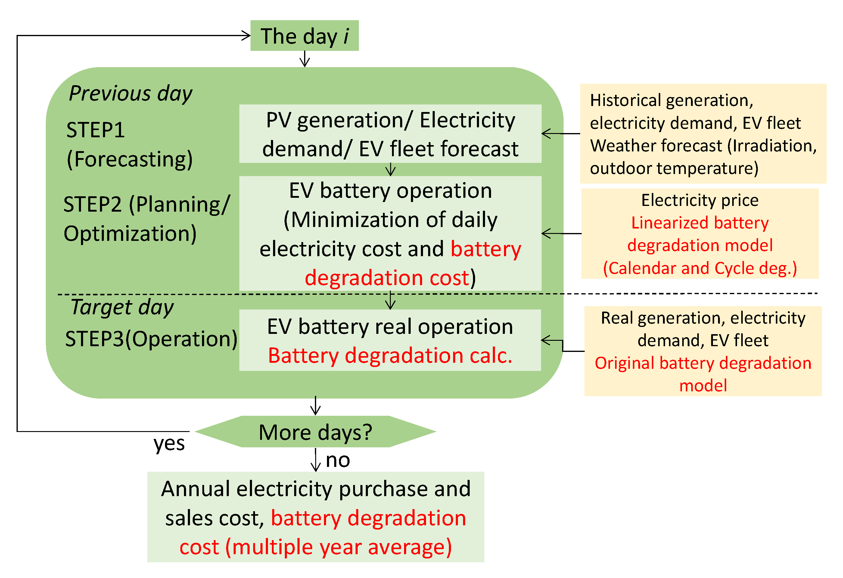
We adopted the degradation model derived by Schmalstieg [6] for an NMC battery, which is commonly used as an EV battery. In this model, calendar and cycle aging were separately modeled, and the parameters of the model were quantitatively described. The framework of this study is shown in Figure 1. A linearized battery degradation model was incorporated into the optimization model in the planning step in the EV DR estimation model, and the original detailed nonlinear model was used in the final cost calculation in the operation step.
Furthermore, an EV DR evaluation model was proposed and analyzed to minimize the electricity rates and degradation costs affected by ambient temperature, battery SOC, and DOD.
The contribution of this paper can be summarized as follows:
- The battery degradation model is combined with the EV DR evaluation model to evaluate the degradation cost due to additional charge/discharge operations.
- By modeling the degradation factors of the battery by dividing them into calendar degradation and cycle degradation, the relationship between each factor and the operation method can be clearly evaluated.
- The EV DR evaluation model uses EV fleet data using a Monte Carlo simulation based on the actual EV utilization and offers a realistic evaluation.
Our EV DR evaluation model is based on charge and discharge control based on hourly driving demand and residential electricity demand for arbitrage under assumed electricity tariffs and does not cover shorter time interval controls such as frequency control.
3. Battery Degradation Model
Generally, battery degradation is evaluated based on the highest value when comparing the capacity fade and power fade. Most of the previous studies have already addressed capacity fade degradation. Therefore, we also calculated the degradation cost due to capacity degradation based on the degradation model derived by Schmalstieg [6]. The NMC model [6] is a holistic aging model that uses an impedance electric–thermal mode based on an accelerated aging test set, which consists of more than 60 cells of a commercial high-energy 18650 system with NMC cathode material. Both calendar and cycle aging were separately evaluated in the model.
In the proposed EV DR evaluation model, the degradation is modeled as the sum of calendar and cycling aging (Equation (1)), because it is easy to linearize.
The original calendar and cycle aging models were linearly approximated for the optimization step in the EV DR estimation model, as described below.
3.1. Calendar Aging
𝐿𝑐𝑎𝑙 was modeled based on the elapsed time, cell temperature, and the secondary open-circuit voltage (OCV), which determines the SOC in the NMC model [6]. The OCV–SOC correlation is shown in Figure 1.
By making the appropriate modifications, the degradation model can be rewritten based on 𝛳𝑇 and 𝛳𝑆𝑂𝐶.
Here, 𝛳𝑇 is the calendar degradation coefficient due to temperature, and 𝛳𝑆𝑂𝐶 is the calendar degradation coefficient due to SOC at the reference temperature (25 °C).
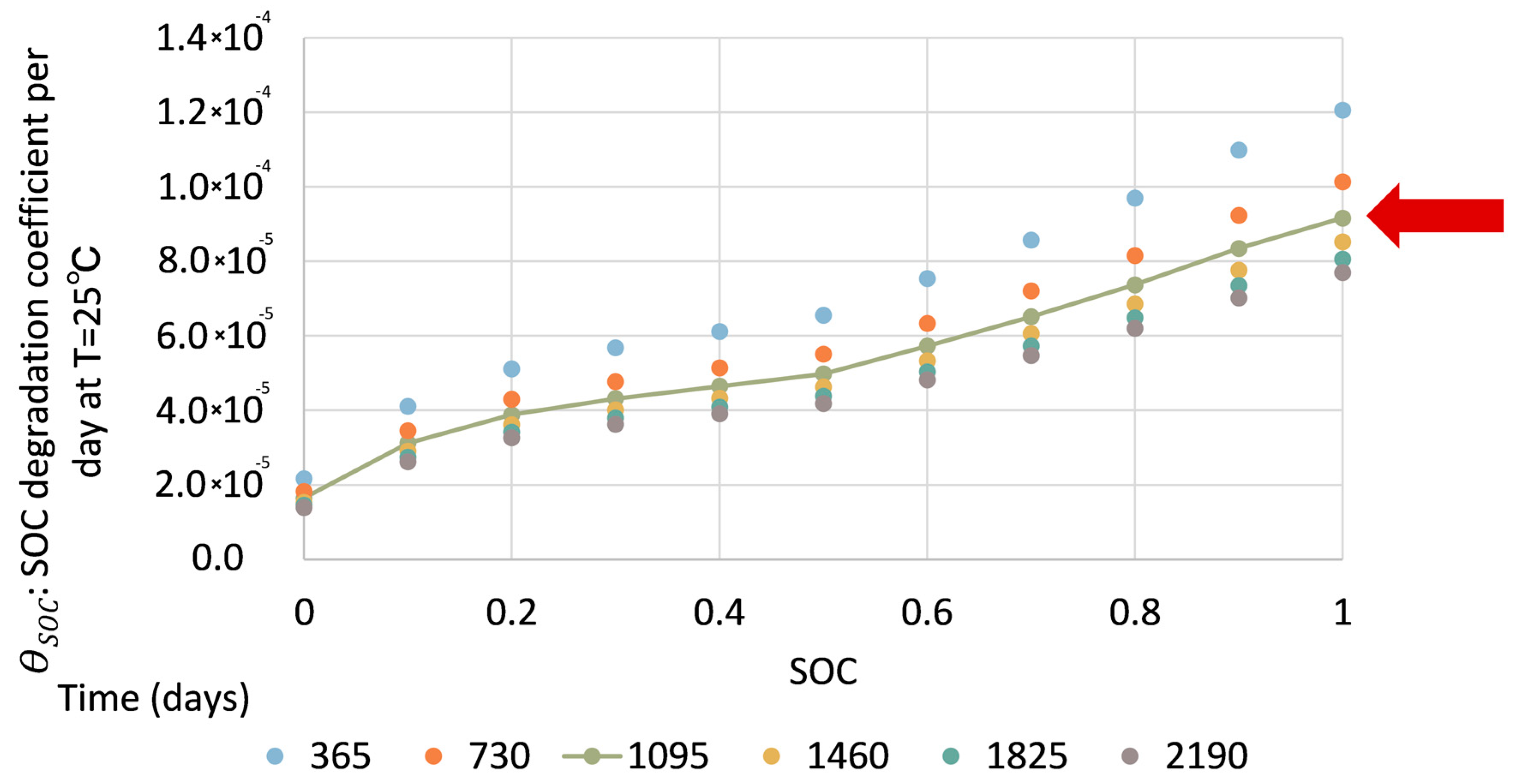
Figure 2 shows the contribution of the SOC to the degradation, which is called SOC degradation and is obtained from Equations (2) and (3) at the reference temperature. Here, V in Equation (3) was calculated through the linear interpolation of the plot in Figure 3. SOC degradation, when the elapsed time was 1090 days (3 years), which was assumed to be half of the battery life, was adopted as the average SOC degradation model, which was approximated by a linear piecewise interpolation. We assumed that the battery life was 6 years based on the information of the actual value of the warranty period of 5 to 8 years for in-vehicle batteries. To obtain the temperature degradation coefficient, Equation (3) was modified, and 𝛳𝑇 was plotted as a function of 𝑇 minus 𝑇𝑟𝑒𝑓 and fitted as an exponential curve, as shown in Figure 4.
Here, 𝑇𝑟𝑒𝑓 is the reference cell temperature (25 °C).
The cell temperature of an EV battery is primarily affected by a cooling device. Although some previous models considered the transient behavior due to the difference between the cell and environment temperatures, in this study, it was assumed that the cell temperature is equal to the environment temperature, as was the case in [18]. Furthermore, in this work, the temperature degradation at 15 °C was used for situations in which the temperature was lower or equal to 15 °C.
3.2. Cycling Aging
Lcyc is firstly modeled by Equations (6) and (7) based on V and DOD, as indicated in [6]:
where Q is the energy throughput (EFC), which is the number of cycles required for the accumulation of the number of Ampere-hours stored in the battery. Q equals 1 at a one-cycle operation of 100% DOD.
In our model, the influence of SOC (V) in cycle aging was neglected to simplify the model. As a result, cycle degradation was evaluated based only on DOD in the optimization stage. Cycle aging was linearly approximated, as in Equation (8), for optimization in the EV DR estimation model.
where 𝛳dod is the linearized DOD degradation coefficient per EFC for cycling aging. Figure 5 quantifies the contributions of each parameter by showing the cycle degradation obtained with Equations (6) and (7), when EFC = 1000 and DOD = 10%. When the SOC contribution is greater than or equal to 20%, the cycle degradation increases with SOC. As storage batteries usually operate under this condition, the reduction of SOC basically leads to the reduction of cycle aging. Furthermore, a lower SOC is preferred in the optimization model for the influence of SOC regarding calendar aging, and the impact of the neglect of SOC degradation regarding cycle aging is considered to be small in terms of optimization.
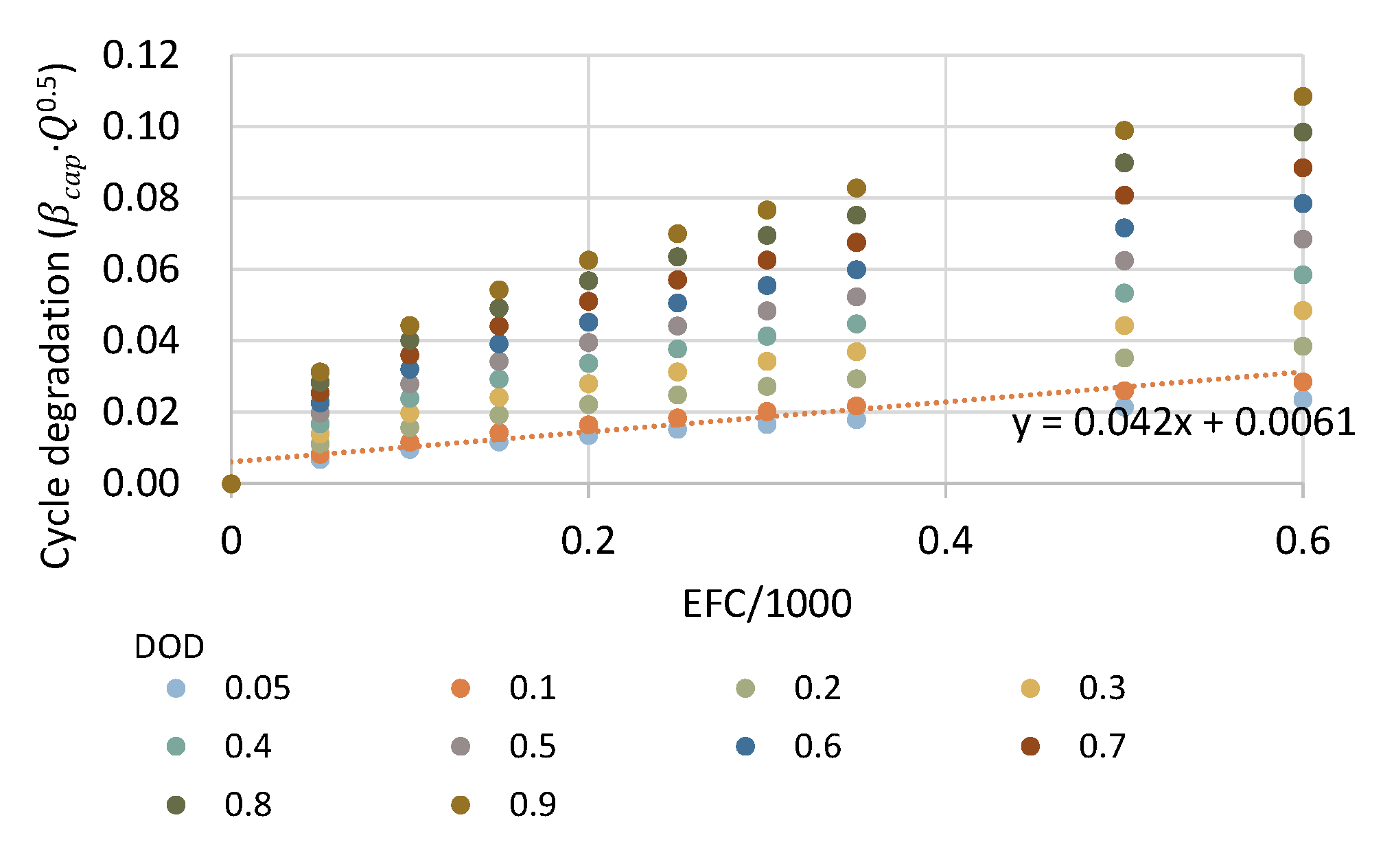
Figure 6 shows the behavior of EFC concerning cycle degradation for multiple values of DOD. The linear approximation was performed when EFC values ranged between 0 and 600. As a result, a 𝛳dod value of 0.042 was obtained for the degradation per 1000 EFC when DOD was equal to 10%. This DOD value was assumed because the purpose of our V2G model was to reduce electricity costs, and the charge/discharge output was as small as 3 kW for a capacity of 40 kWh. Furthermore, as the annual EFC was approximately 100 when charge/discharge control was performed for various driving patterns in a previous study conducted with a driving simulator [3], the targeted range was set to 600 EFC, which is equivalent to six years of battery life. At the operational stage in the EV DR estimation model, in which the daily battery operation on the target day including the prediction error was analyzed, the degradation cost was calculated, using Equations (2),(3),(6),(7), considering that SOC was not neglected during the evaluation of cycle aging. Finally, the effects of all factors were considered. As the duration of the cycle for driving EV is shorter than 1 h, the EFC is expected to increase, resulting in increased degradation. The proposed 1-h model does not consider the impact of the driving cycle, as this study focused on analyzing the impact on the predictability of the degradation caused by additional cycles for V2G for arbitrage. As a result, the cycle degradation calculated by the proposed model was lower than the actual value.
4. EV DR Evaluation Model Considering Battery Degradation
We have already proposed an EV DR model to evaluate the effects of EV batteries in households with a PV power generation system [3]. That model was improved in this work to account for battery degradation, as shown in Figure 9. The control variables were the power purchased from and sold to the grid, and the charge and discharge operations of the EV battery. This model consisted of three steps, namely forecasting, planning on the previous day, and operation on the target day, and the series of procedures was repeated for 1 year.
In this work, the information in red letters in Figure 9 was added to the process to consider battery degradation. In the planning stage, the degradation cost was added to the objective variable, and the linearized degradation model was added to the constraint conditions. The operation of the battery was optimized to achieve the minimum cost. In the operation stage, the operation of the EV battery was conducted based on the plan in the previous step, actual PV power generation, and actual EV availability, and the degradation cost was calculated from the original model shown in Equations (2), (3), (6) and (7). The following are the optimization methods for the planning stage and the rules for the operational stage.
4.1. EV Battery Optimization Model (Planning Model)
The formulation, including the degradation cost, used in the optimization of the planning stage is shown in Equations (9)–(28), in which the highlighted terms and expressions were added to account for the degradation cost. In the daily optimization model, the number of control variables and expressions are 600 and 443, respectively. The variables starting with “x” are the control variables, and all are continuous real variables, except for , and , which are binary variables.
Objective functions:
Subject to
| 𝑡 | time (1–24) |
| 𝑖 | number of intervals used in the linear approximation (1–10) |
| 𝑥𝑐𝑎𝑙(𝑡), 𝑥𝑐𝑦𝑐(𝑡) | calendar degradation rate (%), cycle degradation rate (%) |
| 𝑥𝑑𝑜𝑑(𝑡) | DOD (%) |
| 𝑏𝑝(𝑖) | interval step used in the linear approximation (0.1–1.0) |
| 𝑠𝑑𝑒𝑔𝑣𝑎𝑙(𝑖) | SOC degradation rate at SOC level 𝑖 |
| 𝑥𝑠𝑜𝑐𝑑𝑢(𝑖, 𝑡) | SOC level dummy variable (0 or 1) |
| 𝑥𝑠𝑜𝑐𝑑𝑒𝑔(𝑡) | SOC degradation rate |
| 𝜃𝑇 | temperature degradation coefficient (= 0.9725e0.0728⊿T) |
| 𝜃𝑑𝑜𝑑 | DOD degradation coefficient (= 0.042/1000EFS) |
| 𝑝𝑑𝑒𝑔 | unit cost of capacity degradation (US cents/%). |
EVs can be charged or discharged from the power grid when at home, and when outside the home, they can be charged at external charging stations (CSs) when the battery SOC is below the lower limit. In this work, we assumed that the electricity price at the CS was higher than at home, where the charging task was mainly conducted. Constraint Equations (10)–(21) were originally proposed by [3], and Equations (22)–(24) describe the relationship between SOC and the calendar degradation rate. The SOC degradation curve used had an elapsed time of 1090 days (3 years), as previously illustrated in Figure 2, and it was linearly approximated with 10 intervals as “𝑠𝑑𝑒𝑔𝑣𝑎𝑙.” Equations (25) and (26) were used to calculate the DOD. Equation (27) describes the calendar degradation rate based on the temperature and SOC, and Equation (28) describes the cycle degradation rate based on the DOD.
4.2. Operating Model on the Target Day
The daily power used in the charge/discharge task was determined according to the preset rules based on actual PV power generation demand, actual EV status, and the optimization model in Section 4.1, coupled with the planned charge/discharge. The resulting degradation cost was calculated based on the battery condition during the operation stage using Equations (2),(3),(6),(7). As the degradation rate was initially large and nonlinear, the six-year average degradation rate was used to calculate the approximate degradation cost.
5. Simulation
5.1. Simulation Conditions
Table 1 shows the three EV operation scenarios covered in this work. The EV night charging case, in which the EV is charged at midnight when the electricity is relatively inexpensive, was the reference for the comparison between the results of the different scenarios. According to previous simulation results [3] that did not consider the degradation cost, the user-free case, in which the forecast of the EV driving and the PV power generation were not required, was more economical than the user input case.
The simulation cases and the data used in the simulations are shown in Table 2 and Table 3. In the nighttime charging and user-free cases that did not require the forecast and planning process, the reference SOC was assumed to be relatively high (0.8) to avoid the risk of running out of battery charge. To be consistent with that assumption, in the user setting case, the reference SOCs for the charging only control and charging/discharging control were set to 0.8 and 0.5, respectively. We simulated the impact of EV battery utilization for 10 PV-owned all-electric detached houses using three types of driving patterns and using a driving simulator for 8760 h (see Figure 10) [3]. Figure 10 shows the average stay probability and mileage per hour obtained from 100 simulations based on the state transition data of real vehicles with three representative driving patterns.
The assumptions of battery capital cost and residual value have a significant effect on the results. The remaining value after battery degradation depends on whether it can compete with the new storage battery price at that time. Assuming that the battery capital cost is US$15,000 and the lithium-ion battery price reduction rate over six years is 40% based on the Bloomberg NEF forecast [19], the residual value when using up to 80% of capacity in 6 years is calculated as follows:
15,000 × 80% × (1–40%) = 7200 (US $)
Here, the degradation cost due to the 1% capacity degradation of the battery is calculated as follows:
(15,000–7200)/20%/100 = 390 (US $/%)
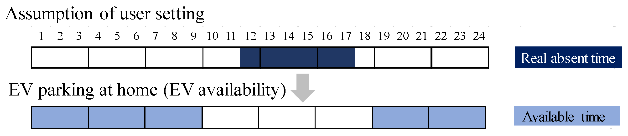
Figure 11.
Setting of EV available time in the user input case.

5.2. Simulation Results
Figure 12 and Figure 13 show the simulation results of each case described in Table 2 using driving pattern 2, in which the driving mileage and the periods at home are classified as average. Figure 12 indicates the annual total cost, which includes the purchase cost from the utility, PV surplus selling cost (negative), and calendar and cycle degradation costs, considering the average of 10 households. Figure 13 indicates the changes in the total cost, with and without degradation cost, compared to that of the nighttime charge (case 1). The results of the battery degradation model combined with the battery price and life assumptions adopted in this study indicated that the ratios of the calendar and cycle degradation costs to the total cost were 29.3% and 4.3%, respectively, for nighttime charging (case 1). Calendar degradation was more dominant. Keeping SOC as low as possible and reducing the charge/discharge cycles may lead to the suppression of battery degradation. This conclusion is supported by previous literature and shows that a lower SOC is dominant for degradation costs, and it is more economical to maintain a lower SOC status until just before the consumer’s use of the vehicle [15,20].
The battery employed in case 2-3, in which a charge/discharge control was used, had a lower SOC than that used in case 2-1, in which a charge only control was employed, resulting in a lower calendar degradation. By contrast, case 2-3 had a higher cycle degradation than that in case 2-1 because of an increase in the number of charge and discharge cycles. For each case, the total cost was slightly reduced when the degradation cost was added to the optimization target. The cost reductions when the degradation cost was considered in the EV DR evaluation model were, respectively, $8.2 and $2.7 for the charge only control and the charge and discharge control, obtained by the difference between the costs of cases 2-1 and 2-2, and 2-3 and 2-4. This change was small because the daily optimization-based model, in which the SOC at the end of the day must be equal to or greater than the initial reference value, had a small SOC variation, as shown in Figure 14. As a result, the optimization results were not significantly different when the degradation was added, leading to a negligible gain in economic efficiency.
The user-free cases (3-1 and 3-2), in which planning and optimization steps were not conducted, became less economical than the respective user input cases (2-1 and 2-3) when the battery degradation cost was considered. They were more economical than the user input cases when the battery degradation cost was not considered [3], and the effect of considering battery degradation led to the opposite result. This conclusion was achieved as cases 3-1 and 3-2 required relatively high SOC to fulfill the safety assumption made in the previous section.
The user input charge control in case 2-1 cost $40 more than that in the base case (case 1). The poorer economic efficiency occurred because of the increase in the calendar degradation cost, which exceeded the reduction of the purchase cost due to charging from PV cells. This increase in calendar degradation cost was attributed to the SOC reference value and operation methods. Even if the reference SOC is the same as 0.8, the EV SOC will be higher in case 2-1 than in case 1 due to the difference in the operation method, as shown in Figure 14. The battery was charged so that the SOC becomes the reference value of 0.8 after 23:00 in case 1, whereas it was charged so that the SOC is over the reference value of 0.8 by 23:00 of the last planning time in the case 2-1. This is because it is assumed that the battery was charged so that the SOC becomes the reference value of 0.8 after 23:00 in the base case, whereas it was charged so that the SOC is over the reference value of 0.8 by 23:00 of the last planning time in the case of the charge control 2-1 as shown in Figure 15. Regarding case 2-3 of the charge/discharge control, a cost reduction of $417 was achieved when compared to the cost of case 1. If the SOC can be kept low, the purchased cost from the utility can be greatly reduced, and the calendar degradation cost can be suppressed even if cycle degradation increases.
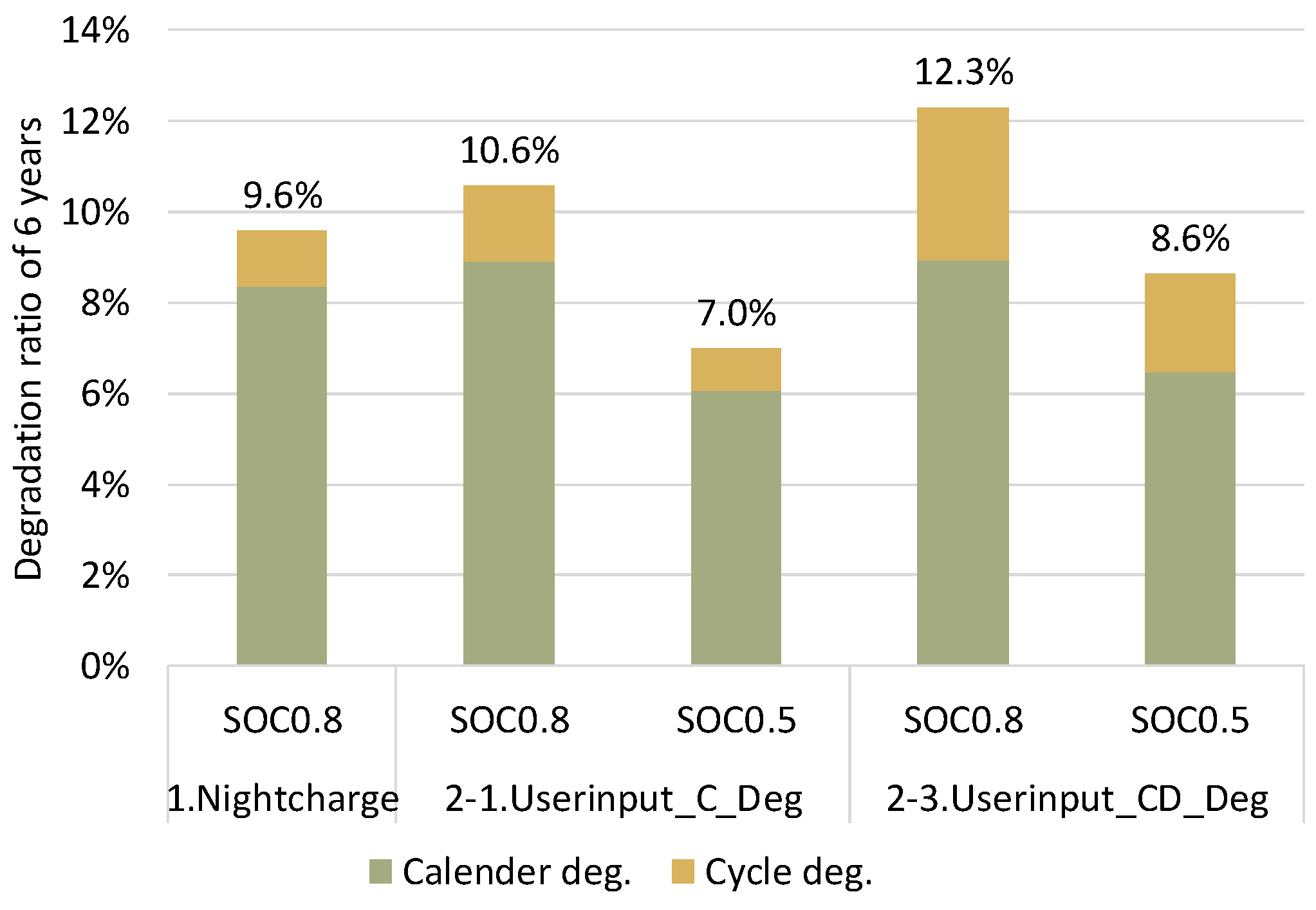
Figure 16 shows the total degradation rate for driving pattern 2 by accumulating the degradation costs over six years, assuming the same one-year operating results for each year. By comparing cases 1 and 2-1, the degradation ratio of case 2.1 was 1 percentage point higher than that of case 1 (nighttime charge) because of the higher average SOC. Furthermore, the cycle degradation was higher when compared to that of the base case, as the cycle degradation was dependent on the SOC function, as shown in Equations (6) and (7). If the reference SOC was 0.5, the degradation ratio could be reduced to 7%. Regarding case 2.3, the degradation ratio was significantly larger than that of the base case when the reference SOC was 0.8. By contrast, this value was reduced to 8.6% when the reference SOC was 0.5. The frequent charge and discharge cycles could not be modeled for actual EV driving, as the period in which each model simulation was conducted (hourly) was not small enough. Therefore, the actual cycle degradation is expected to be higher than that shown in Figure 16, as described in Section 3.2.
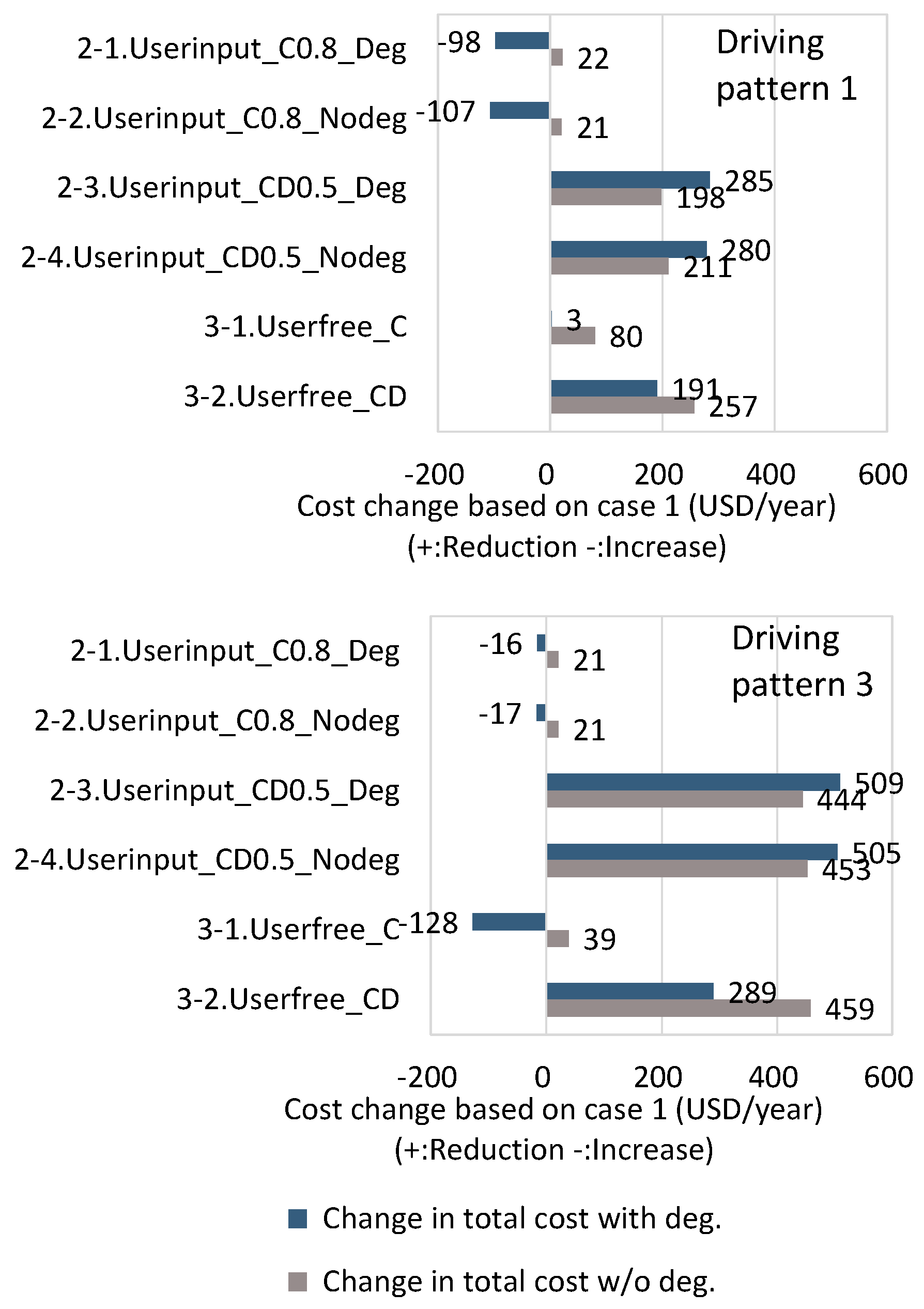
The results obtained when different driving patterns were used are shown in Figure 17. The cost in the charge control case was increased by US$98 when compared to the base case. Furthermore, the cost due to the charge and discharge control was reduced by US$285 for driving pattern 1, in which the driving mileage was high and the staying periods were short. Regarding driving pattern 3, in which the driving mileage was low and the staying periods were long, the cost in the charge control case was increased by $16 compared to the base case, but the cost in the charge and discharge control case was reduced by US$509. As the availability of batteries at the residence of the user was relatively high, longer staying periods led to a greater cost advantage for the charge and discharge control cases.
Considering case 2-1 with a reference SOC of 0.5, the cost reductions were US$165, 194, and 204 (compared with the base case), respectively, when driving patterns 1, 2, and 3 were used, indicating that a large cost reduction is possible if the SOC is low. Regarding the base case, if the reference SOC was 0.5 at night, the degradation cost was greatly reduced, but the cost of external charging at the charge stations occurred when driving pattern 1 was applied. In the user input case, the charging and discharging plan was developed to minimize external charging even if the reference SOC was low. In this case, the user needs to set the staying time and the number of miles traveled while driving, and the planned and operation stages are necessary when control is employed. However, because the SOC can be kept low, and the charging and discharging tasks are executed at the appropriate time in the user input case, the cost can be significantly reduced.
6. Conclusions
In this study, an EV demand response evaluation model that considers EV battery degradation was proposed. The degradation model of NMC batteries proposed in previous research was incorporated into the optimization and operation model for EV charge and discharge control. Furthermore, the degradation cost was evaluated from the residual value of the battery.
The total cost, including battery degradation, was evaluated considering the charging and discharging control strategy based on the settings inputted by the user. Furthermore, the results were compared with a base case called the night operation case. As a result, the SOC significantly influenced the degradation cost of the daily operation of the battery. If the SOC could be kept low, a significant cost reduction could be expected. Moreover, the user-free cases, in which forecasting or planning steps were not conducted, were more economical than the controlled cases when the degradation cost was not considered, but their cost increased when the degradation costs were added.
In addition, the analysis of each driving pattern showed that the cost was reduced when the mileage was low and the staying time was long. Furthermore, there was no significant difference in the cost evaluation by adding the degradation cost to the EV DR evaluation model, as the SOC at the end of the day could not be lower than the reference value.
In the future, we are planning to combine the proposed model with different battery degradation models and to evaluate the effects of setting each parameter of the residual value of the battery and the electricity tariff structure.
Author Contributions
Conceptualization, Y.I. and K.O.; methodology, Y.I.; software, Y.I.; validation, Y.I.; data curation, Y.I.; writing—original draft preparation, Y.I.; writing—review and editing, Y.I.; visualization, Y.I.; supervision, K.O. All authors have read and agreed to the published version of the manuscript.
Funding
This research was funded by JST CREST under Grant JPMJCR15K4, Japan.
Conflicts of Interest
The authors declare no conflict of interest.
Nomenclature
| 𝐿𝑐𝑎𝑝 | battery degradation capacity |
| 𝐿𝑐𝑎𝑙 | battery calendar degradation |
| 𝐿𝑐𝑦𝑐 | battery cycling degradation |
| 𝑇 | cell temperature (k) |
| 𝑑𝑎𝑦 | elapsed time (days) |
| 𝑉 | open-circuit voltage (v) |
| 𝛳𝑆𝑂𝐶 | calendar degradation coefficient due to soc at the reference temperature |
| 𝛳𝑇 | calendar degradation coefficient due to temperature |
| 𝑇𝑟𝑒𝑓 | reference cell temperature (k) |
| 𝑄 | equivalent full cycles (efc) |
| 𝐷𝑂𝐷 | depth of discharge |
| 𝑡 | time (1–24) |
| 𝑖 | number intervals used in the linear approximation (1–10) |
| 𝑥𝑏𝑢𝑦 (𝑡) | electricity purchased at time t of the optimization model (kWh/h) |
| 𝑥𝑠𝑒𝑙𝑙 (𝑡) | electricity sold at time t of the optimization model (kWh/h) |
| 𝑥𝑐𝑠 (𝑡) | electricity purchased at charge stations at time t of the optimization model (kWh/h) |
| 𝑥𝑐h (𝑡) | electricity charged at time t of the optimization model (kWh/h) |
| 𝑥𝑑𝑖𝑠 (𝑡) | electricity discharged at time t of the optimization model (kWh/h) |
| 𝑥𝑠𝑜𝑐 (𝑡) | battery SOC at time t of the optimization model (kWh) |
| 𝑥𝑐h𝑑𝑢𝑚 (𝑡) | dummy variable denoting the charge time in the optimization model |
| 𝑥𝑑𝑖𝑠𝑑𝑢𝑚 (𝑡) | dummy variable denoting the discharge time in the optimization model |
| 𝑥𝑐𝑎𝑙 (𝑡) | calendar degradation rate (%) at time t in the optimization model (kWh/h) |
| 𝑥𝑐𝑦𝑐 (𝑡) | cycle degradation rate (%) at time t of the optimization model (kWh/h) |
| 𝑥𝑑𝑜𝑑 (𝑡) | DOD at time t in the optimization model |
| 𝑏𝑝 (𝑖) | interval step used in the linear approximation (0.1–1.0) |
| 𝑠𝑑𝑒𝑔𝑣𝑎𝑙 (𝑖) | SOC degradation rate at SOC level 𝑖 |
| 𝑥𝑠𝑜𝑐𝑑𝑢𝑚 (𝑖, 𝑡) | SOC level dummy variable (0 or 1) |
| 𝑥𝑠𝑜𝑐𝑑𝑒𝑔 (𝑡) | SOC degradation rate |
| 𝜃𝑇 | temperature degradation coefficient |
| 𝜃𝑑𝑜𝑑 | DOD degradation coefficient |
| 𝑝𝑏𝑢𝑦 (𝑡) | the purchase price of the electricity price at time t (US cents/kWh) |
| 𝑝𝑠𝑒𝑙𝑙 (𝑡) | the selling price of the electricity at time t (US cents/kWh) |
| 𝑝𝑐𝑠 (𝑡) | purchase price of the electricity at charge stations at time t (US cents/kWh) |
| 𝑓𝑙 (𝑡) | predicted EV fleet at time t (km) |
| 𝑑𝑒𝑚 (𝑡) | predicted electricity demand at time t (kWh/h) |
| 𝑝𝑣 (𝑡) | predicted PV power generation at time t (kWh/h) |
| 𝑝𝑑𝑒𝑔 | unit cost of capacity degradation (US cents/%) |
| h𝑜𝑚𝑒 (𝑡) | predicted index on whether EV is staying at home at time t (1: stay, 0: out) |
| 𝐵𝑘𝑊h𝟢 | initial battery SOC (kWh) |
| 𝑀 | sufficiently large constant (=10,000) |
| 𝑏𝑢𝑦 (𝑡) | final electricity purchased at time t (kWh/h) |
| 𝑠𝑒𝑙𝑙 (𝑡) | final electricity sold at time t (kWh/h) |
| 𝑐𝑠 (𝑡) | final electricity purchased at charge stations at time t (kWh/h) |
| 𝑐h (𝑡) | final electricity charged at time t (kWh/h) |
| 𝑑𝑖𝑠 (𝑡) | final electricity discharged at time t (kWh/h) |
| 𝑠𝑜𝑐 (𝑡) | final battery SOC at time t (kWh/h) |
| 𝑓𝑙𝑟𝑒𝑎𝑙 (𝑡) | real EV fleet at time t (km) |
| 𝑑𝑒𝑚𝑟𝑒𝑎𝑙 (𝑡) | real electricity demand at time t (kWh/h) |
| 𝑝𝑣𝑟𝑒𝑎𝑙 (𝑡) | real PV power generation at time t (kWh/h) |
| 𝜂𝑐h | battery charge efficiency |
| 𝜂𝑑𝑖𝑠 | battery discharge efficiency |
| 𝐸𝑉𝑒𝑓𝑓 | EV fleet efficiency (km/kWh) |
| 𝐵𝑘𝑊 | battery inverter capacity (kW) |
| 𝐵𝑘𝑊h𝑚𝑎𝑥 | upper limit of battery capacity (kWh) |
| 𝐵𝑘𝑊h𝑚𝑖𝑛 | lower limit of battery capacity (kWh) |
References
- Agency, I.E. Global EV Outlook 2019. In Scaling-Up the Transition to Electric Mobility; IEA: London, UK, 2019. [Google Scholar] [CrossRef]
- Iwafune, Y.; Ogimoto, K.; Azuma, H. Integration of Electric Vehicles into the Electric Power System Based on Results of Road Traffic Census. Energies 2019, 12, 1849. [Google Scholar] [CrossRef] [Green Version]
- Iwafune, Y.; Ogimoto, K.; Kobayashi, Y.; Murai, K. Driving Simulator for Electric Vehicles Using the Markov Chain Monte Carlo Method and Evaluation of the Demand Response Effect in Residential Houses. IEEE Access 2020, 8, 47654–47663. [Google Scholar] [CrossRef]
- Thompson, A.W. Economic implications of lithium ion battery degradation for Vehicle-to-Grid (V2X) services. J. Power Source 2018, 396, 691–709. [Google Scholar] [CrossRef]
- Ben-Marzouk, M.; Chaumond, A.; Redondo-Iglesias, E.; Montaru, M.; Pélissier, S. Experimental Protocols and First Results of Calendar and/or Cycling Aging Study of Lithium-Ion Batteries–the MOBICUS Project. World Electr. Veh. J. 2016, 8, 388–397. [Google Scholar] [CrossRef] [Green Version]
- Schmalstieg, J.; Käbitz, S.; Ecker, M.; Sauer, D.U. A holistic aging model for Li(NiMnCo)O2 based 18650 lithium-ion batteries. J. Power Sources 2014, 257, 325–334. [Google Scholar] [CrossRef]
- Wang, J.; Purewal, J.; Liu, P.; Hicks-Garner, J.; Soukazian, S.; Sherman, E.; Sorenson, A.; Vu, L.; Tataria, H.; Verbrugge, M.W. Degradation of lithium ion batteries employing graphite negatives and nickel–cobalt–manganese oxide + spinel manganese oxide positives: Part 1, aging mechanisms and life estimation. J. Power Sources 2014, 269, 937–948. [Google Scholar] [CrossRef]
- Smith, K.; Wood, E.; Santhanagopalan, S.; Kim, G.-H.; Pesaran, A. Advanced Models and Controls for Prediction and Extension of Battery Lifetime. In Proceedings of the Large Lithium Ion Battery Technology & Application Symposia Advanced Automotive Battery Conference, Atlanta, GA, USA, 4 February 2014. [Google Scholar]
- Xu, B.; Oudalov, A.; Ulbig, A.; Andersson, G.; Kirschen, D.S. Modeling of Lithium-Ion Battery Degradation for Cell Life Assessment. IEEE Trans. Smart Grid 2018, 9, 1131–1140. [Google Scholar] [CrossRef]
- Marongiu, A.; Roscher, M.; Sauer, D.U. Influence of the vehicle-to-grid strategy on the aging behavior of lithium battery electric vehicles. Appl. Energy 2015, 137, 899–912. [Google Scholar] [CrossRef]
- Wang, D.; Coignard, J.; Zeng, T.; Zhang, C.; Saxena, S. Quantifying electric vehicle battery degradation from driving vs. vehicle-to-grid services. J. Power Sources 2016, 332, 193–203. [Google Scholar] [CrossRef] [Green Version]
- Neubauer, J.; Wood, E. The impact of range anxiety and home, workplace, and public charging infrastructure on simulated battery electric vehicle lifetime utility. J. Power Sources 2014, 257, 12–20. [Google Scholar] [CrossRef]
- Hoke, A.; Brissette, A.; Maksimovic, D.; Pratt, A.; Smith, K. Electric vehicle charge optimization including effects of lithium-ion battery degradation. In Proceedings of the IEEE Vehicle Power and Propulsion (VPPC), Colorado, CO, USA, 6–9 September 2011. [Google Scholar] [CrossRef]
- Ortega-Vazquez, M.A. Optimal scheduling of electric vehicle charging and vehicle-to-grid services at household level including battery degradation and price uncertainty. IET Gener. Transm. Distrib. 2014, 8, 1007–1016. [Google Scholar] [CrossRef]
- Uddin, K.; Jackson, T.; Widanage, W.D.; Chouchelamane, G.; Jennings, P.A.; Marco, J. On the possibility of extending the lifetime of lithium-ion batteries through optimal V2G facilitated by an integrated vehicle and smart-grid system. Energy 2017, 133, 710–722. [Google Scholar] [CrossRef]
- Dubarry, M.; Devie, A.; McKenzie, K. Durability and reliability of electric vehicle batteries under electric utility grid operations: Bidirectional charging impact analysis. J. Power Sources 2017, 358, 39–49. [Google Scholar] [CrossRef]
- Uddin, K.; Dubarry, M.; Glick, M.B. The viability of vehicle-to-grid operations from a battery technology and policy perspective. Energ. Policy 2018, 113, 342–347. [Google Scholar] [CrossRef]
- Smith, K.; Earleywine, M.; Wood, E.; Neubauer, J.; Pesaran, A. Comparison of Plug-In Hybrid Electric Vehicle Battery Life Across Geographies and Drive Cycles. In Proceedings of the 2012 SAE World Congress and Exhibition, Detroit, MI, USA, 24–26 April 2012. [Google Scholar] [CrossRef] [Green Version]
- BloombergNEF A Behind the Scenes Take on Lithium-ion Battery Prices. Available online: https://about.bnef.com/blog/behind-scenes-take-lithium-ion-battery-prices/ (accessed on 22 May 2020).
- Das, R.; Wang, Y.; Putrus, G.; Kotter, R.; Marzband, M.; Herteleer, B.; Warmerdam, J. Multi-objective techno-economic-environmental optimisation of electric vehicle for energy services. Appl. Energy 2020, 257, 113965. [Google Scholar] [CrossRef]
Figure 1.
Framework of this study.

Figure 2.
State of charge (SOC) degradation coefficient per day versus SOC at 25 °C for calendar degradation.
Figure 2.
State of charge (SOC) degradation coefficient per day versus SOC at 25 °C for calendar degradation.

Figure 3.
Open-circuit voltage versus the state of charge at 35 °C [6].
Figure 3.
Open-circuit voltage versus the state of charge at 35 °C [6].

Figure 4.
Temperature degradation coefficient approximation for calendar degradation.

Figure 5.
Cycle degradation over SOC at 1000 equivalent full cycles (EFC) and 10% depth of discharge (DOD).
Figure 5.
Cycle degradation over SOC at 1000 equivalent full cycles (EFC) and 10% depth of discharge (DOD).

Figure 6.
Cycle degradation over EFC by DOD.

Figure 7.
Battery capacity degradation when charging/discharging once a day (cell temperature, 25 °C; DOD, 10%; and SOC, 90%).
Figure 7.
Battery capacity degradation when charging/discharging once a day (cell temperature, 25 °C; DOD, 10%; and SOC, 90%).

Figure 8.
Battery capacity degradation when charging/discharging once a day (cell temperature, 25 °C; DOD, 10%; and SOC, 50%)
Figure 8.
Battery capacity degradation when charging/discharging once a day (cell temperature, 25 °C; DOD, 10%; and SOC, 50%)

Figure 9.
Structure of the electric vehicle demand response (EV DR) evaluation model considering battery degradation.
Figure 9.
Structure of the electric vehicle demand response (EV DR) evaluation model considering battery degradation.

Figure 10.
Annual average staying time ratio and mileage in the driving pattern data of three EVs.

Figure 12.
EV battery operation results in driving pattern 2 (10-house average of annual cost).

Figure 13.
EV battery operation results with driving pattern 2 (10-house average of annual cost change for case 1).
Figure 13.
EV battery operation results with driving pattern 2 (10-house average of annual cost change for case 1).

Figure 14.
EV battery SOC status for cases 2-3 and 2-4 in January, with household using driving pattern 2 for 1 week.
Figure 14.
EV battery SOC status for cases 2-3 and 2-4 in January, with household using driving pattern 2 for 1 week.

Figure 15.
EV battery SOC status for the base case, charge control with degradation (reference SOC = 0.8 (32 kWh)), and charge control with degradation (referenced SOC = 0.5 (20 kWh)) cases in January, with household using driving pattern 2 for 1 week.
Figure 15.
EV battery SOC status for the base case, charge control with degradation (reference SOC = 0.8 (32 kWh)), and charge control with degradation (referenced SOC = 0.5 (20 kWh)) cases in January, with household using driving pattern 2 for 1 week.

Figure 16.
EV battery degradation ratio for 6 years for each case in driving pattern 2.

Figure 17.
The 10-house average of annual cost change based on the base case of case 1 in driving patterns 1 and 3.
Figure 17.
The 10-house average of annual cost change based on the base case of case 1 in driving patterns 1 and 3.


Table 1.
EV operation case.
| EV Operation Case | Operation Method | Need for Forecast and Planning |
|---|---|---|
| EV night charging (base case) | The battery is charged to the reference SOC only at nighttime when the electricity is cheap | No |
| User input case | The EV available time (the presence or absence at home in 8 periods by 3 hours) and the daily travel distance (upper-limit input in 10 km increments) are set by the user at 23:00 on the previous day, as shown in Figure 11. The daily battery operation is planned considering that the SOC at 23:00 on the target day is above the reference SOC. | Yes |
| User-free case | For the charge only control, the battery is charged up to the maximum capacity when PV surplus power is available and charged up to the reference SOC during the nighttime electricity rate period. For the charge/discharge control, the battery is discharged up to the reference SOC to supply the electricity demand that exceeds the PV generation during the daytime electricity rate period. The charging operation is the same as that for the charge only control. | No |
Table 2.
Case setting.
| Case ID | EV Operation Case | Control Method | Reference SOC of Battery | Optimization with Degradation Cost |
|---|---|---|---|---|
| 1 | EV night charging (base case) | Charge | 0.8 | - |
| 2-1 | User input case | Charge only | 0.8 | Yes |
| 2-2 | Charge only | 0.8 | No | |
| 2-3 | Charge and discharge | 0.5 | Yes | |
| 2-4 | Charge and discharge | 0.5 | No | |
| 3-1 | User-free case | Charge only | 0.8 (Charged during nighttime) 1.0 (Charged with surplus PV) | - |
| 3-2 | Charge and discharge | 0.8 (Charged during nighttime) 1.0 (Charged with surplus PV) 0.5 (Discharged when the EV is at the residence of the user) | - |
Table 3.
Parameter setting.
| Parameter | Value |
|---|---|
| Electricity price | The purchase price at the residence of the user: 18/33 US cents/kWh (nighttime 23:00–7:00/other time 7:00–23:00) Selling price: 8 US cents/kWh The purchase price at CSs: 50 US cents/kWh |
| Demand and PV generation profile | Data measured for 8760 h in 10 all-electric houses (PV generation 5000–6200 kWh/yr., demand other than hot water supply 6100–8400 kWh/yr.) |
| EV | Battery capacity: 40 kWh Charge and discharge capacity: 3 kW SOC lower limit: 20 kWh at V2H periods in the user-free case and 8 kWh in other cases EV fleet efficiency: 7 km/kWh Battery charge and discharge efficiency: 90% each |
Publisher’s Note: MDPI stays neutral with regard to jurisdictional claims in published maps and institutional affiliations. |
© 2020 by the authors. Licensee MDPI, Basel, Switzerland. This article is an open access article distributed under the terms and conditions of the Creative Commons Attribution (CC BY) license (http://creativecommons.org/licenses/by/4.0/).
Share and Cite
MDPI and ACS Style
Iwafune, Y.; Ogimoto, K. Economic Impacts of the Demand Response of Electric Vehicles Considering Battery Degradation. Energies 2020, 13, 5771. https://0-doi-org.brum.beds.ac.uk/10.3390/en13215771
AMA Style
Iwafune Y, Ogimoto K. Economic Impacts of the Demand Response of Electric Vehicles Considering Battery Degradation. Energies. 2020; 13(21):5771. https://0-doi-org.brum.beds.ac.uk/10.3390/en13215771
Chicago/Turabian StyleIwafune, Yumiko, and Kazuhiko Ogimoto. 2020. "Economic Impacts of the Demand Response of Electric Vehicles Considering Battery Degradation" Energies 13, no. 21: 5771. https://0-doi-org.brum.beds.ac.uk/10.3390/en13215771
Note that from the first issue of 2016, this journal uses article numbers instead of page numbers. See further details here.