Deep Learning Approach to Power Demand Forecasting in Polish Power System


1
Faculty of Electronics, Military University of Technology, ul. gen. S. Kaliskiego 2, 00-908 Warsaw, Poland
2
Faculty of Electrical Engineering, Warsaw University of Technology, pl. Politechniki 1, 00-661 Warsaw, Poland
*
Author to whom correspondence should be addressed.
Energies 2020, 13(22), 6154; https://0-doi-org.brum.beds.ac.uk/10.3390/en13226154
Submission received: 12 October 2020
/
Revised: 12 November 2020
/
Accepted: 19 November 2020
/
Published: 23 November 2020
(This article belongs to the Special Issue Computational Intelligence and Load Forecasting in Power Systems)
Abstract
:The paper presents a new approach to predicting the 24-h electricity power demand in the Polish Power System (PPS, or Krajowy System Elektroenergetyczny—KSE) using the deep learning approach. The prediction system uses a deep multilayer autoencoder to generate diagnostic features and an ensemble of two neural networks: multilayer perceptron and radial basis function network and support vector machine in regression model, for final 24-h forecast one-week advance. The period of the data that is the subject of the experiments is 2014–2019, which has been divided into two parts: Learning data (2014–2018), and test data (2019). The numerical experiments have shown the advantage of deep learning over classical approaches of neural networks for the problem of power demand prediction.
1. Introduction
The stability of the electric power system is the most important factor in power delivery. It is guaranteed by the balance between electric load and supply. With the help of accurate electric load forecasting, electric power operators can adjust the electric supply according to real-time forecasted load and maintain the normal operation of electric power systems. An accurate 24-h forecast for the next few days is very important for the operation of national power grids, both technically and economically [1,2,3,4].
This problem has drawn attention from many researchers in different fields, and many forecasting methods have been developed in the past [4,5,6,7]. The most important problem is to propose the optimal set of diagnostic features that are used as the input attributes in the final regression network [8]. The development of artificial intelligence methods and machine learning has accelerated the progress in designing systems, which better reflect the nonlinear features of electric loads. Multilayer perceptron (MLP), radial basis function network (RBF), support vector machine in regression model (SVR), and random forest (RF) have been widely used in the process of prediction of the changes of electric loads [4,5].
Huang et al. [8] proposed an RF-based feature selection method, and then an improved RF regression model was trained using features selected by a sequential backward search method. Moon et al. [4] have proposed a prediction system by combining an RF model and MLP model to predict the daily electric loads. A strategy for short-term load forecasting by using SVR in regression model has been proposed in [1].
The paper of Yang et al. [9] has studied the application of an ensemble of predictors to improve the accuracy of short-term electricity demand forecasting. The combination of neural networks, neuro-fuzzy ANFIS, and differential SARIMA has been presented. The paper of Correia et al. [10] has presented multi-model methodology for forecasting the sales of liquefied petroleum gas cylinders. The problem of sensitivity and accuracy in the ensemble of predictors has been considered in the paper of Fernandez et al. [11]
In recent years deep learning techniques have attracted great interest in many branches of engineering applications, including short time series prediction [12,13,14,15,16,17]. Unlike traditional machine learning, the deep learning approach extracts features directly from data without the manual intervention of the human operator. The deep neural networks include multiple hidden layers between the input and the output. They are strictly responsible for the generation of a limited number of diagnostic features, as well as characterizing the raw input data.
The paper of Liu et al. [6] has shown the application of stacked denoising autoencoder for short-term load forecasting, taking into account such factors as historical loads, somatosensory temperature, relative humidity, and daily average loads. Only the daily average power demand was of interest in final forecasting tasks.
He [13] has integrated multiple types of input features by using appropriate neural network components. The convolutional neural network components were used to extract features from the historical load sequence, and the recurrent neural model was used to reconstruct the implicit dynamics within these data.
Tian C et al. [7] and Kang et al. [17] have proposed long short-term memory (LSTM) and convolutional neural network for short-term load forecasting, showing their superiority in time series prediction problems. Deep learning has shown its superiority. The study of sensitivity versus accuracy of the ensemble integrated by weighting methodologies, such as majority voting, simple averaging, and winner takes all, have been presented.
Merkel et al. [16] compared the effectiveness of various forecasting methods in load forecasting of natural gas, including a linear regression model, a shallow MLP, and two deep networks of different sizes. It was found that, in general, the deep network outperforms other methods.
This paper also deals with applying deep learning to load forecasting in the power system. However, we propose a significantly different approach to the forecasting problem. First, the 24-h load data of the entire week form the basis of the input signals in the system. The input size of such a vector is 170 (168 h and 2 bits indicating the season), and the autoencoder is then used to process this vector to create the diagnostic features of reduced dimension, that can well characterize the load for the entire week. The encoder application is a clever tool to compress the long input vector to its efficient code of much shorter length. This reduces the complexity of the circuit, resulting in a better generalization capability. The diagnostic features generated by the autoencoder represent the input attributes for the ensemble of two neural networks: Multilayer perceptron and radial basis function network, and support vector machine. The results predicted by these three nets are merged to produce a final forecast for the next week (24-h forecasts for seven days). This is the most important difference to most papers devoted to short term load forecasting, where only the next day 24-h load pattern is predicted. The numerical experiments performed on the Polish Power System (PPS) data have shown the improved performance of the proposed solution.
2. Database
The proposed prediction system will be tested on the database of the PPS of the last six years [18]. According to the PPS, the total capacity of power installed in the System, on 31 December 2019 was 46,799 MW. The national mean demand for power for 2019 was 23,451 MW, and the maximal demand 26,504 MW.
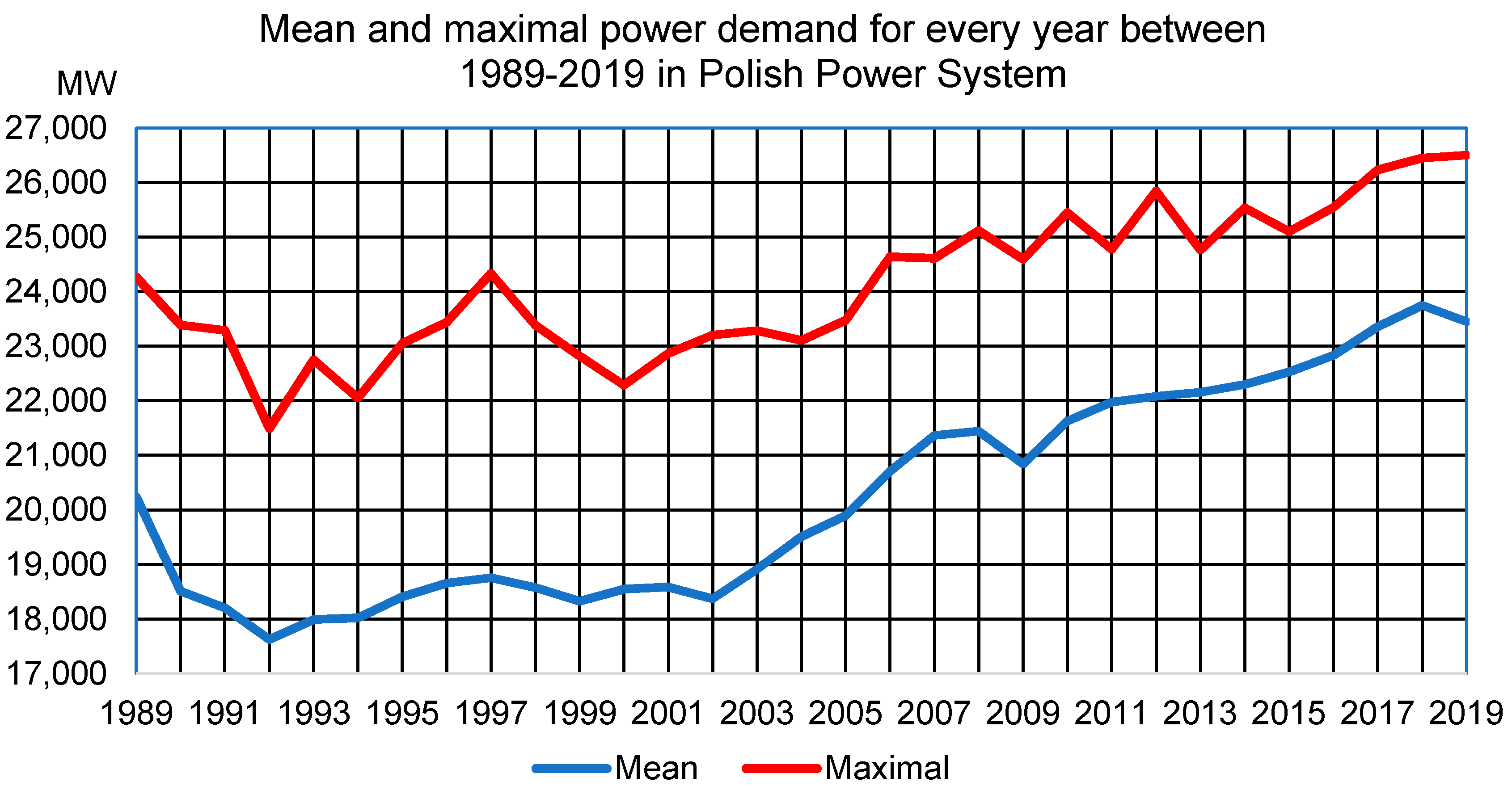
The 30-year changes in mean and maximal power demand are presented in Figure 1. Analyzing the values only for the period of the last six years, it can be said that the mean power demand in 2019 was increased by 5.16% in comparison to 2014 and maximal power demand by 3.79% in this period. The values from this mentioned six-year period, year to year, are presented in Table 1.
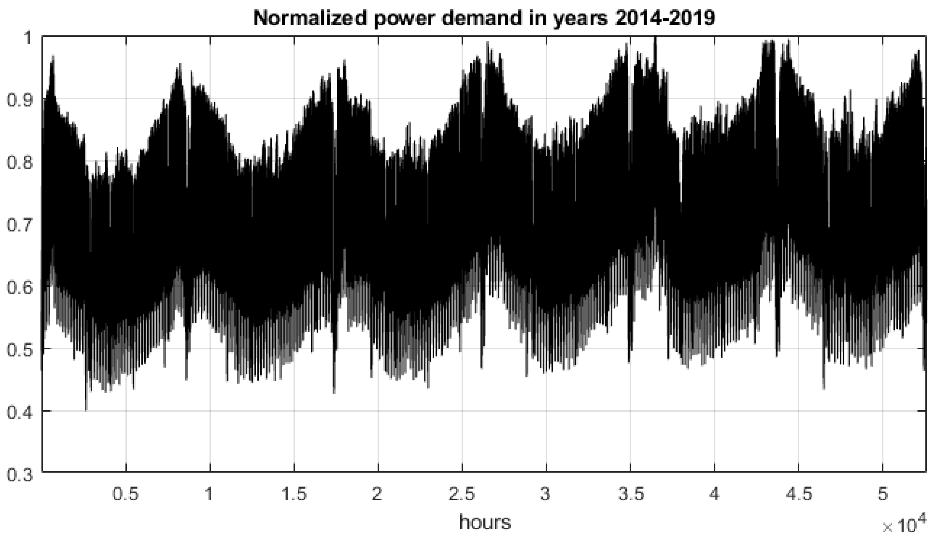
The hourly load data for the Polish power supply system used in numerical experiments were collected over six years: 2014–2019. The period covers 2191 days (52,584 hourly load data). The data were normalized by the maximum value. Their distribution is presented in Figure 2.
The normalized data were divided into seven-day partitions, covering the whole weeks. They started from the 1st January 2014. The number of partitions (weeks) is 313, where 261 weeks were used in learning, and 52 weeks—for testing. Every partition contains 168 load data, representing hourly loads. Two bits representing the season, coded in a binary way: Winter (11), spring (01), summer (00), autumn (10), were added to each partition.
So that learning and testing vectors, serving as input attributes, contain 170 elements. These data processed in the learning system contain redundant information and a significant portion of the noise. Their direct application as the input signals to neural predictors will lead to a decrease in the accuracy of forecast in testing mode. Therefore, there is a need to reduce the data dimension by extracting only the representative diagnostic features.
Different approaches to feature selection have been proposed in the past: Application of genetic algorithms, a random forest of decision trees, Fisher criterion, different statistical hypothesis methods, stepwise fit selection, etc. [19,20]. These methods analyze the importance of particular elements of the input attribute vector and pass them or stop as the diagnostic features. The other approach is to formulate the weighted mixture of the original input attributes and reduce the number of such mixtures to the proper size. The most typical methods of this type belong to principal component analysis (PCA) or linear discriminant analysis (LDA) [19,21]. Both methods represent a linear approach to the reduction problem of the data dimension.
In this work, we propose applying a deep autoencoder in the role of a diagnostic feature generator [22]. Autoencoder may be treated as a multilayer nonlinear generalization of PCA. The data processing is done layer by layer with a reduced number of neurons in the succeeding layers. In this way, the system is forced to compress the input information, by representing it by the smaller and smaller size vectors.
In contrary to the solutions, presented in many papers devoted to loading forecasting, we deal with a 24-h prediction for the seven days of the week (one-week advance). The input information delivered to the autoencoder covers the data of the whole week (168 load data and two bits of the season). This vector of 170 elements will be reduced by an autoencoder to the size, which provides the best results of the predicted load demands for the whole next-week days.
3. Autoencoder Based Forecasting System
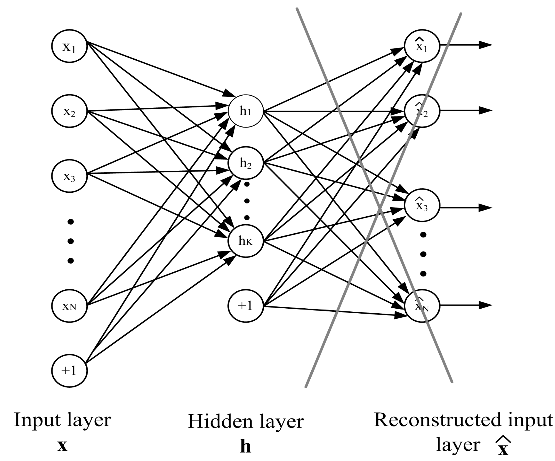
Normalized hourly load demands and 2 bits representing seasons can be considered as original input attributes, which are subject to reduction. The aim is to represent the original data by smaller dimensions, however, well-representing load characteristics of the week power curve. Thanks to such reduction, the complexity of the system is reduced, which results in better generalization ability. This task was done in our work by autoencoder [21,22] (Figure 3).
Autoencoder is a neural solution that processes input data via hidden layers. The succeeding hidden layers apply reduced dimensions concerning input data. In the learning process, the encoder subnetwork projects input data into coded data represented by vector h = f(x) of reduced dimension. The decoder part makes reverse mathematic operation trying to reconstruct the input data with specified accuracy [22], where g represents the activation function vector chosen by the user.
The learning process in creating each of the hidden layers may be defined as an adaptation of its weights, which leads to the minimization of the cost function E defined as follows
where x(k) represents the input signal vector, N is the size of this vector, and p is the number of observations. For better generalization capacity of the network, the additional regularization is applied, which takes into account minimization of weights, the sensitivity of hidden neurons to minor changes in input signal values, as well as specialization of neurons in particular areas of input data [22]. This is an important advantage of autoencoder over other deep learning solutions, for example, CNN [17], in which such regularization is not provided.
After finishing the learning procedure, the reconstructing part of the autoencoder is eliminated from the structure, and the hidden layer signals provide the input to the next stage of dimensionality reduction. In this way, the autoencoder attempts to encode the input data by using fewer and fewer hidden neurons whose weights are adjusted to allow an acceptable reconstruction of the input data. It is an auto-associative way of learning.
The signals of the succeeding layers of the autoencoder represent the diagnostic features of the analyzed data. The deeper the layer, the most reduced is its dimension. The last layer of the autoencoder represents input attributes that will be used as the final set of the diagnostic features for the real neural predictor.
Note that in contrast to the classical approach, where the characteristics of data are generated using the expert-based method, the data characterization in this method is generated by an automatic self-organizing process without human experience-based intervention. In our work, the learning process of auto-coding was implemented in the programming environment of Matlab [21]. The different number of hidden layers and neurons have been tried in experiments. The best generalization ability of the system was achieved by using two hidden layers. The number of neurons in these layers was selected by additional experiments.
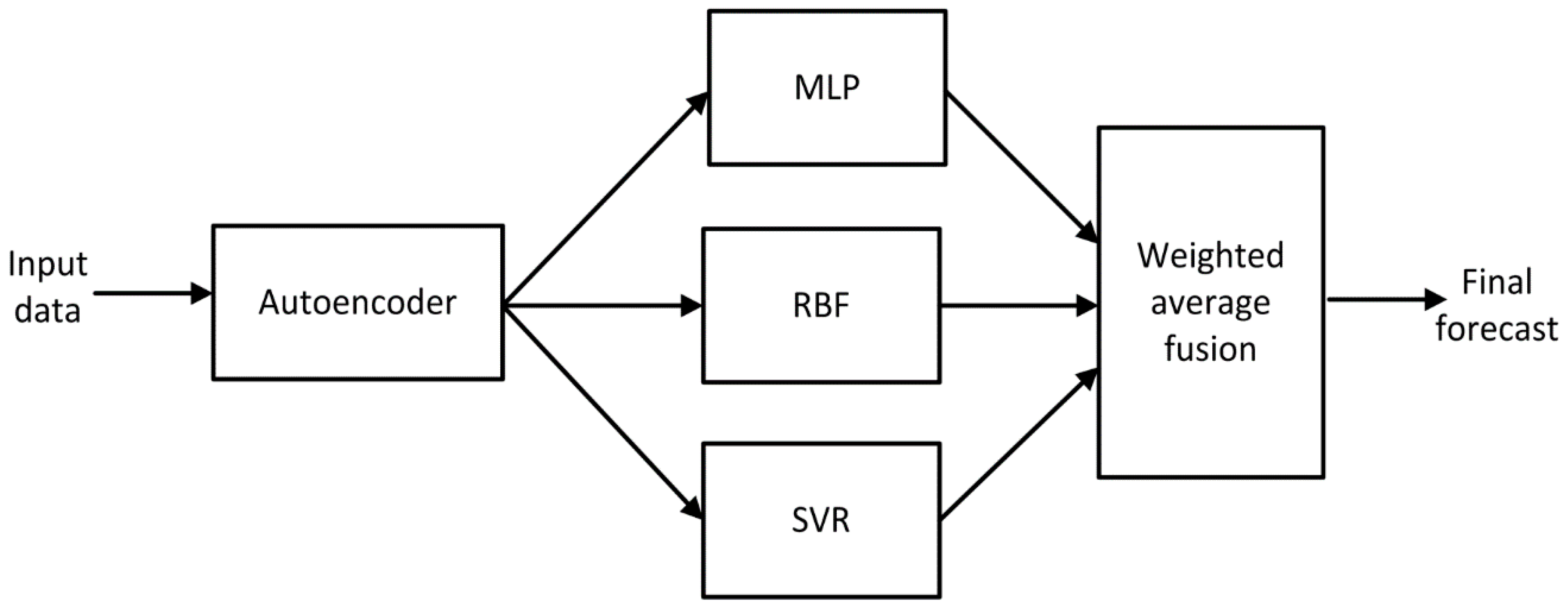
The signals of the last hidden layer are treated as the diagnostic features, which are put to the input of three networks: Multilayer perceptron, radial basis function network, and support vector machine with Gaussian kernel, working in regression mode. These three units form the members of the forecasting ensemble. The general structure of the whole system is presented in Figure 4.
The final decision of an ensemble is elaborated by weighted averaging the forecasts predicted by its three members. To make the performance of ensemble members more independent, the learning data of each individual members were generated randomly from the whole learning set by assuming its population 90% of the learning set.
4. Results of Experiments
The experiments have been conducted using the data of the PPS of six years (2014–2019). The first five years, 2014–2018, have been used in the learning stage, and 2019 was left for testing only. The structure of different elements of the forecasting system should have been analyzed and researched. The first task was to find the optimal autoencoder structure, especially the number of layers, as well as the number and activation of neurons in individual layers, which provide the most accurate forecast results. The experiments have shown that particular neural networks perform best for a varying number of features.
In the next stage, the optimal structure and parameters of neural networks have to be defined. They include the number of neurons in MLP, the number of centers in RBF, as well as the kernel function type and parameters of the kernel function, and the regularization parameters in SVR. In the last step, the results generated by individual neural networks of the ensemble are integrated into one result for obtaining a final forecast, hopefully of better accuracy than individual predictors. The fusion procedure was based on a weighted average of the results provided by these three predictors for a particular 24 h of the seven days of the next week. The prediction of power demand for hth hour of the particular day is estimated using the following formula,
where M = 3, wi(h) is the weight associated with ith predictor for hth hour, and pi(h) is the power demand for hth hour forecasted by the ith predictor. The value of the weights wi(h) is estimated based on the accuracy of the prediction of the ith neural predictor in the learning stage. This value was defined by considering the accuracy η of ith predictor for hth hour of the day,
The exponent m may take any value emphasizing the dominance of the most accurate unit of an ensemble. We have applied value m = 244, which was found as the best one.
4.1. MLP Network
The conducted research has shown the remarkable dependence of forecast accuracy on the applied autoencoder structure, especially the number of diagnostic features (the population of neurons in the last hidden layer), the parameter choice of the network used for forecasting, etc. Different models of autoencoders have been investigated. The best one was two hidden layer model with a linear activation function. Table 2 presents the dependence of forecasting results of MLP cooperating with the structure of autoencoder applying a different number of hidden neurons. The results are presented as mean absolute percentage error (MAPE) [19,20] for all testing data (2019) not taking part in learning.
Analyzing the data from Table 2, it is evident that the most accurate results of MLP predictor (1.96% of MAPE) have been obtained at 80 neurons in the first and 40 neurons in the second hidden layer of an autoencoder and for 14 sigmoidal neurons in a hidden layer of MLP network of 168 output neurons (the signals representing 24-h forecast for the seven days of the week).
4.2. RBF Network
The second network applied in an ensemble was the RBF network. This solution uses Gaussian activation functions, therefore, the network represents the local approximation character. Its performance is strictly dependent on the number of hidden Gaussian neurons and their parameters (center and width of function). The learning procedure was split into two phases: Determination of centers by using K-means clusterization and singular value decomposition (SVD) applied in output weights adaptation. The introductory experiments have been performed to find the best structure of the whole system.
The results of these experiments in the form of MAPE on testing data for some chosen numbers of Gaussian neurons and predefined structure of autoencoder are shown in Table 3. The best accuracy was obtained using 100 and 50 neurons in hidden layers of an autoencoder and 50 Gaussian neurons in the RBF network. The applied width of the Gaussian function was σ = 0.7. The best MAPE testing error, in this case, was 1.47% for the whole of 2019.
The best results were obtained using 100 and 50 neurons in the autoencoder and 50 centers of the RBF network. The use of a smaller number of centers, e.g., 30, has decreased accuracy.
4.3. Support Vector Machine
The last member of the ensemble was a support vector machine in regression mode. This network differs from the previous two by a completely different learning procedure. Thanks to a special form of nonlinear mapping (here Gaussian kernel) of the input data into multidimensional space, it is possible to transform the regression task to the classification problem solved by quadratic programming. The important hyper-parameters that should be adjusted before the learning phase are parameter γ of the Gaussian kernel , regularization constant C, and tolerance value ε. These parameters have been adjusted in the introductory phase of experiments, shown in Table 4. The table presents some testing results for a different choice of these predefined parameters.
The most accurate results have been obtained now for autoencoder structure, which was the same as for RBF 170-100-50. However, the MAPE achieved was higher compared with the RBF network.
4.4. Ensemble of Neural Networks
The last stage of the forecasting procedure is fusing the results of particular individual predictors into the final forecast. This was done by applying the weighted average procedure described in the previous section. The important is the choice of exponent m in definition (3). A high value of this exponent prefers the strongest team unit when establishing the final forecast. A small value leads to a more even influence of the individual predictors. Table 5 illustrates this phenomenon using different values of m in the calculation of weights. The higher value of the exponent amplifies more accurate forecasts to the less accurate. Assuming the MAPE errors for individually acting neural networks, as shown in Table 2, Table 3 and Table 4, we get the appropriate accuracies ηi as follows: ηRBF = 0.9853, ηMLP = 0.9804 and ηSVR = 0.9756, and the weights wi presented in Table 5.
If the value m = 1 is chosen, all weights are very similar, and each predictor has a similar effect on the final prognosis. If we choose m = 300, we get significantly different effects of the individual members of the ensemble. In this case, the predictor that was the best in learning mode (here RBF network) is dominant.
Table 6 presents the values of weights obtained based on average accuracy in learning for 24-h out of 5 years (2014, 2015, 2016, 2017, 2018). They are given for all three neural networks forming the ensemble. Due to the highest accuracy of RBF, the weights corresponding to this predictor dominate for all 24 h. However, the second-highest weight differs for different hours. For example, for hours 1–18 and 22–24, MLP is better, and for hours 19, 20, and 21, the SVR is more important.
Table 7 shows the effect of choosing different values of exponent m on the total MAPE error of the ensemble. The best forecast accuracy results in the testing data (2019) were obtained at the application of m = 244. The mean MAPE error for 2019 was then reduced to the value of 1.428% from the best 1.47% obtained by the RBF predictor. As it is seen, the choice of the value of m is very significant. The not proper choice may lead to a reduction of accuracy of the ensemble to the best individual member.
Table 8 presents the MAPE testing error for all 52 weeks of 2019. The best forecast was obtained for the 22nd week (29th May–4th June with MAPE = 0.64%) and the worst for the 52nd week (25th–31st December with MAPE = 8.36%), which covers 25th, 26th (Christmas), and 31st of December (New Year’s Eve) with the very uncommon shape of power curve compared to the typical days of the week.
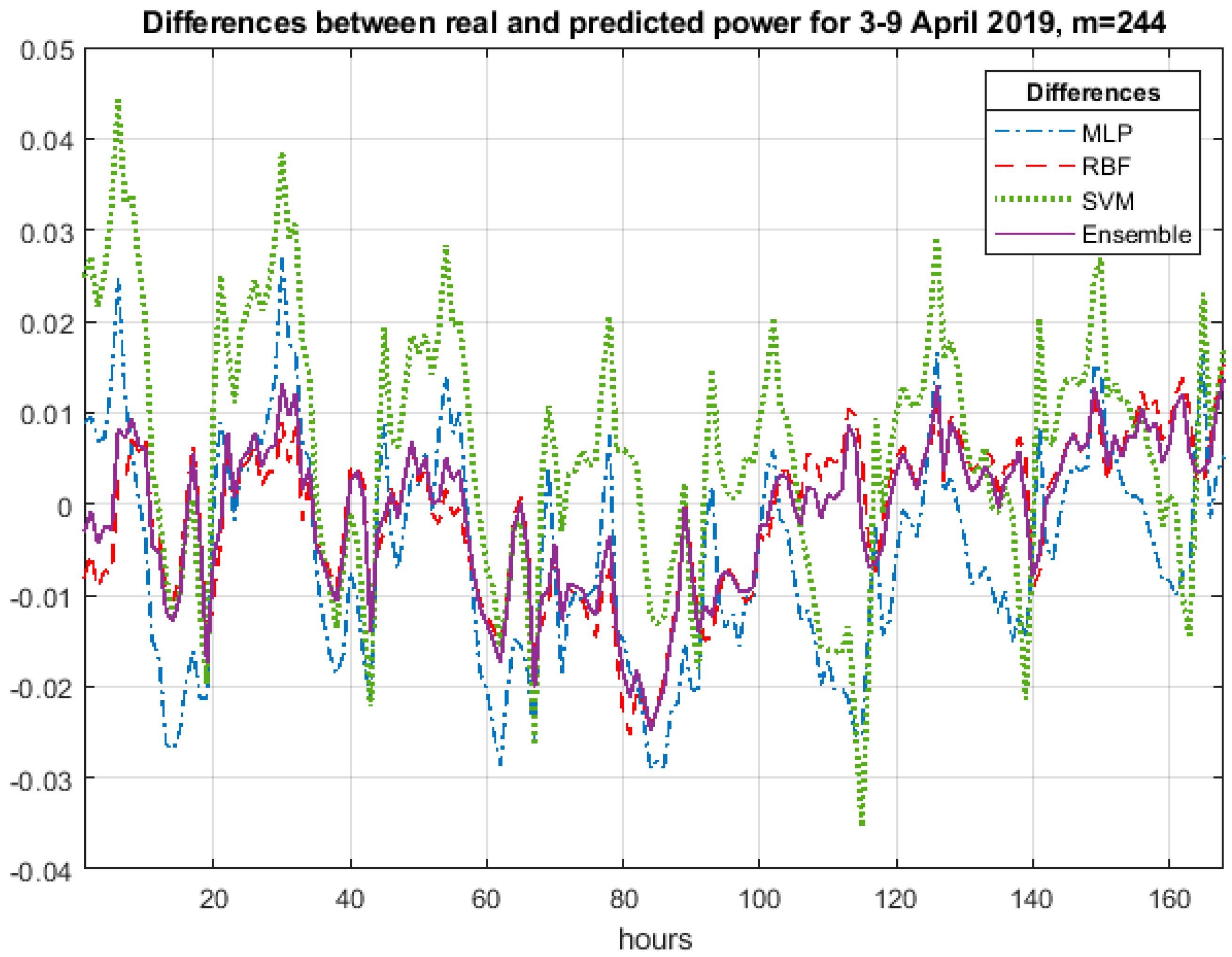
Figure 5 presents the average hourly testing errors for one randomly selected week (3–9 April) of 2019 at the application of exponent m = 244. In most hours, the result of the ensemble follows the best predictor (RBF). This happens when the polarity of errors of the predictors is the same. However, for some hours, different polarity of actual errors committed by the ensemble members can be observed. This provides the field for compensation of error values. These two tendencies: Compensation of different polarity errors and preference of the best predictor, have resulted in a very high value of exponent m.
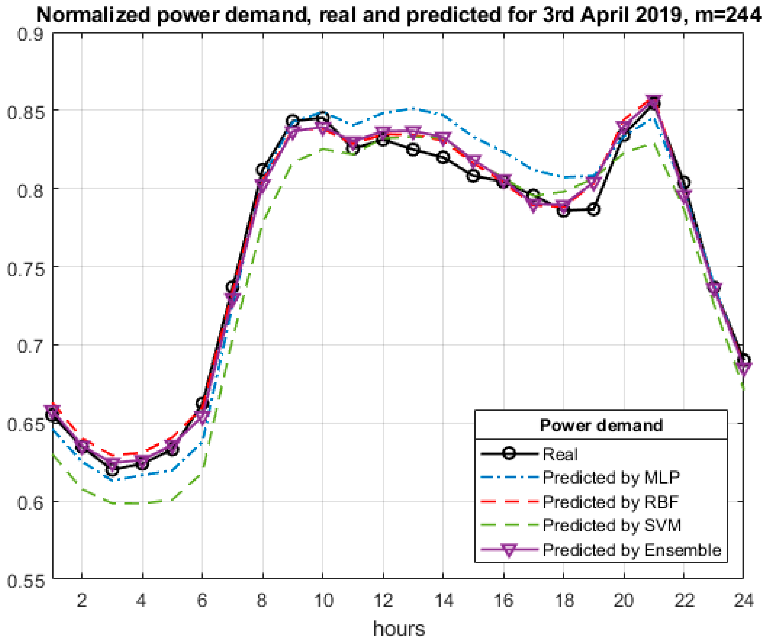
Figure 6 shows the hourly power distribution for the randomly chosen day of 3rd April 2019. In most hourly ranges, the results of ensemble prediction are closest to the real results, however, very close to the best RBF predictor.
The largest discrepancies between the curves are observed for MLP (from 10 to 19 h) and for SVR (from 1 to 10 and from 20 to 22 h).
5. Conclusions
The paper presented the application of deep learning and the ensemble of predictors in predicting the hourly electricity demand in the Polish electricity system. The autoencoder is used as the main tool in developing diagnostic features, serving as input attributes for the three networks: MLP, RBF, and SVR, which are arranged in an ensemble. In contrast to other approaches to load forecasting, the proposed method is based on a weekly perspective. The system generates the hourly power demand for the entire next week (and not for the next day, as in typical classical systems).
The numerical experiments carried out have shown that the sophisticated system of feature generation makes it possible to increase the accuracy of the individual predictors in the one-week forecasts of energy demand. The accuracy achieved with the applied individual predictions was further enhanced by the integrated ensemble based on the weighted average. The improvement was possible by compensating errors committed by individual predictors. The correct value of the exponent used in the weighting coefficients made it possible to obtain better results than the best ensemble member. The final prediction generated by the ensemble takes into account the accuracy of the system in the learning stage, estimated for each hour individually. The experiments have shown that the average MAPE prediction error for all of 2019 has been reduced to a very low value of 1.428%.
It is rather difficult to compare our results to the other presented in the scientific papers. First, the existing approaches are usually limited to the one day ahead forecast for 24 h, while our method is operated on a seven days horizon. Since our system can forecast a 24-h load pattern one week ahead, it solves more complex problems. Furthermore, comparing the results that correspond to the load patterns of different countries is not fair. It is well known that the predictions depend heavily on the complexity of the patterns, which changes considerably for different countries.
The results of our approach may only be objectively compared with the forecast for the PPS (the same complexity of load pattern). For example, the best results (MAPE = 1.73%) were reported for the ensemble predicting the 24-h load pattern on the Polish power grid one day in advance for 2009 [20]. Our best result for the more complex task (seven days in advance) was 1.43%.
It should be noted, that the accuracy of the proposed system is at a level acceptable to the experts working in the electricity markets of our country. Therefore, the method has a certain perspective for practical application.
Future work will focus on applying other deep structures in the time series prediction system and the extension of the ensemble models by using a larger number of different units implementing different prediction mechanisms.
Author Contributions
Conceptualization, S.O. and T.C.; methodology, S.O.; software, T.C. and S.O.; validation, T.C. and S.O.; formal analysis, S.O.; investigation, T.C.; resources, S.O. and T.C.; data curation, T.C.; writing—original draft preparation, T.C. and S.O.; writing—review and editing, S.O. and T.C.; visualization, T.C.; supervision, S.O.; project administration, T.C. and S.O.; funding acquisition, T.C. and S.O. All authors have read and agreed to the published version of the manuscript.
Funding
This research received no external funding.
Conflicts of Interest
The authors declare no conflict of interest.
Abbreviations
The following abbreviations are used in this manuscript.
| KSE | Krajowy System Elektroenergetyczny (Polish Power System) |
| MLP | Multilayer perceptron |
| RBF | Radial basis function |
| SVR | Support vector machine in the regression model |
| MAPE | Mean absolute percentage error |
References
- Ceperic, E.; Ceperic, V.; Baric, A. A strategy for short-term load forecasting by Support Vector Regression Machines. IEEE Trans. Power Syst. 2013, 11, 4356–4364. [Google Scholar] [CrossRef]
- Ding, N.; Benoit, C.; Foggia, G.; Bésanger, Y.; Wurtz, F. Neural network-based model design for short-term load forecast in distribution systems. IEEE Trans. Power Syst. 2016, 31, 72–81. [Google Scholar] [CrossRef]
- Khoshrou, A.; Pauwels, E.J. Short-term scenario-based probabilistic load forecasting: A data-driven approach. Appl. Energy 2019, 238, 1258–1268. [Google Scholar] [CrossRef] [Green Version]
- Moon, J.; Kim, Y.; Son, M.; Hwang, E. Hybrid short-term load forecasting scheme using random forest and multilayer perceptron. Energies 2018, 11, 3283. [Google Scholar] [CrossRef] [Green Version]
- Ciechulski, T.; Osowski, S. Prognozowanie zapotrzebowania na moc w KSE z zastosowaniem grupowania rozmytego. Prz. Elektrotech. 2019, 10, 185–189. [Google Scholar] [CrossRef]
- Liu, P.; Zheng, P.; Chen, Z. Deep learning with stacked denoising auto-encoder for short-term electric load forecasting. Energies 2019, 12, 2445. [Google Scholar] [CrossRef] [Green Version]
- Tian, C.; Ma, J.; Zhang, C.; Zhan, P. A deep neural network model for short-term load forecast based on long short-term memory network and convolutional neural network. Energies 2018, 11, 3493. [Google Scholar] [CrossRef] [Green Version]
- Huang, N.; Lu, G.; Xu, D. A permutation importance-based feature selection method for short-term electricity load forecasting using random forest. Energies 2016, 9, 767. [Google Scholar] [CrossRef] [Green Version]
- Yang, Y.; Chen, Y.; Wang, Y.; Li, C.; Li, L. Modelling a combined method based on ANFIS and neural network improved by de algorithm: A case study for short-term electricity demand forecasting. Appl. Soft Comput. 2016, 49, 663–675. [Google Scholar] [CrossRef]
- Correia, A.; Lopes, C.; Silva, E.C.S.; Monteiro, M.; Lopes, R.B. A multi-model methodology for forecasting sales and returns of liquefied petroleum gas cylinders. Neural Comput. Appl. 2020, 32, 1–27. [Google Scholar] [CrossRef]
- Fernandez, J.C.; Cruz-Ramırez, M.; Hervas-Martınez, C. Sensitivity versus accuracy in ensemble models of artificial neural networks from multi-objective evolutionary algorithms. Neural Comput. Appl. 2018, 30, 289–305. [Google Scholar] [CrossRef]
- Hossen, T.; Plathottam, S.J.; Angamuthu, R.K.; Ranganathan, P.; Salehfar, H. Short-term load forecasting using deep neural networks (DNN). In Proceedings of the 2017 North American Power Symposium (NAPS), Morgantown, WV, USA, 17–19 September 2017; pp. 1–6. [Google Scholar]
- He, W. Load forecasting via deep neural networks. Procedia Comput. Sci. 2017, 122, 308–314. [Google Scholar] [CrossRef]
- Bedi, J.; Toshniwal, D. Deep learning framework to forecast electricity demand. Appl. Energy 2019, 238, 1312–1326. [Google Scholar] [CrossRef]
- Din, G.M.U.; Marnerides, A.K. Short term power load forecasting using deep neural networks. In Proceedings of the 2017 International Conference on Computing, Networking and Communications (ICNC), Silicon Valley, CA, USA, 26–29 January 2017; pp. 594–598. [Google Scholar]
- Merkel, G.D.; Povinelli, R.J.; Brown, R.H. Short-term load forecasting of natural gas with deep neural network regression. Energies 2018, 11, 2008. [Google Scholar] [CrossRef] [Green Version]
- Kang, T.; Lim, D.Y.; Tayara, H.; Chong, K.T. Forecasting of power demands using deep learning. Appl. Sci. 2020, 20, 7241. [Google Scholar] [CrossRef]
- Polish Power System Reports. 2020. Available online: https://www.pse.pl/mapa-raportow (accessed on 4 January 2020).
- Tan, P.N.; Steinbach, M.; Kumar, V. Introduction to Data Mining; Pearson Education Inc.: Boston, MA, USA, 2014. [Google Scholar]
- Siwek, K.; Osowski, S.; Szupiluk, R. Neural network approach for accurate load forecasting in a power system. Appl. Math. Comput. Sci. 2009, 19, 303–315. [Google Scholar] [CrossRef] [Green Version]
- Matlab Manual User’s Guide; MathWorks: Natick, MA, USA, 2019.
- Goodfellow, I.; Bengio, Y.; Courville, A. Deep Learning; MIT Press: Cambridge, MA, USA, 2016. [Google Scholar]
Figure 1.
Mean and maximal power demands in MW, for every year between 1989 and 2019 in the Polish Power System (PPS) [18].
Figure 1.
Mean and maximal power demands in MW, for every year between 1989 and 2019 in the Polish Power System (PPS) [18].

Figure 2.
Normalized power demand in the PPS in the investigated period of 2014–2019.

Figure 3.
The illustration of the learning process of the hidden layer of the autoencoder. The original input vector x is coded into hidden layer signals forming vector h of reduced dimension by applying the auto-association mode in learning. After finishing the learning procedure, the output layer is eliminated, and vector x is represented by reduced size vector h.

Figure 4.
The autoencoder based ensemble system in forecasting the 24-h power demand for the seven days of the next week. Input data is composed of 170-element vectors representing the data of the previous week. The size of these vectors is reduced by an autoencoder to the value dictated by the size of the last hidden layer of it. The output vectors of the autoencoder form the diagnostic features for three solutions of predictors: Neural networks (MLP, RBF) and support vector machine in regression mode, called SVR, which generate the final forecast representing predictions of load demand for the seven days in the next week. The last block performs a fusion of the predicted loads for the particular 24 h of the days within this week.

Figure 5.
The hourly distribution of differences between the actual (real) and predicted power demand for one randomly chosen week 3–9 April 2019 (the results in normalized scale). Total MAPE of this week equal to 0.96%.
Figure 5.
The hourly distribution of differences between the actual (real) and predicted power demand for one randomly chosen week 3–9 April 2019 (the results in normalized scale). Total MAPE of this week equal to 0.96%.

Figure 6.
The distribution of the normalized 24-h power demand for 3rd April 2019, at m = 244. The solid black line represents the real power, and the solid magenta line the forecast made by the ensemble.
Figure 6.
The distribution of the normalized 24-h power demand for 3rd April 2019, at m = 244. The solid black line represents the real power, and the solid magenta line the forecast made by the ensemble.


Table 1.
The mean and maximal power demands in MW for 2014–2019 in Polish Power System.
| Year | Mean Power Demand (MW) | Maximal Power Demand (MW) |
|---|---|---|
| 2014 | 22,301 | 25,535 |
| 2015 | 22,529 | 25,101 |
| 2016 | 22,832 | 25,546 |
| 2017 | 23,357 | 26,231 |
| 2018 | 23,750 | 26,448 |
| 2019 | 23,451 | 26,504 |
Table 2.
Mean MAPE errors for all the weeks of 2019, using MLP network as a predictor.
| MAPE Testing Error of MLP for 2019 | |||
|---|---|---|---|
| Autoencoder Structure | Number of Hidden Sigmoidal Neurons in MLP Network | ||
| 12 | 14 | 16 | |
| 170-60-30 | 2.46% | 2.16% | 2.12% |
| 170-80-40 | 2.36% | 1.96% | 2.15% |
| 170-100-50 | 2.26% | 2.81% | 2.16% |
Table 3.
Mean MAPE errors for all the weeks of 2019, using the RBF network as a predictor.
| MAPE Testing Error of RBF for 2019 | |||
|---|---|---|---|
| Autoencoder Structure | Number of Hidden Radial Neurons in RBF Network | ||
| 30 | 50 | 70 | |
| 170-60-30 | 1.88% | 1.71% | 2.08% |
| 170-80-40 | 1.79% | 1.73% | 2.11% |
| 170-100-50 | 1.69% | 1.47% | 1.58% |
Table 4.
Mean MAPE errors for all the weeks of 2019, using SVR network as the predictor.
| MAPE Testing Error of Gaussian SVR for 2019 γ = 0.05, C = 3000 | |||
|---|---|---|---|
| Autoencoder Structure | Tolerance ε | ||
| 0.003 | 0.006 | 0.015 | |
| 170-60-30 | 3.24% | 3.21% | 3.13% |
| 170-80-40 | 2.61% | 2.61% | 2.68% |
| 170-100-50 | 2.45% | 2.44% | 2.50% |
Table 5.
Weights were obtained based on a Formula (3) using different values of m.
| m | Weights wi | ||
|---|---|---|---|
| RBF | MLP | SVR | |
| 1 | 0.3350 | 0.3333 | 0.3317 |
| 3 | 0.3383 | 0.3333 | 0.3284 |
| 10 | 0.3500 | 0.3330 | 0.3170 |
| 100 | 0.5052 | 0.3069 | 0.1879 |
| 300 | 0.7840 | 0.1757 | 0.0403 |
Table 6.
Weights obtained based on the Formula (3), for m = 244, based on learning error for average 24-h.
Table 6.
Weights obtained based on the Formula (3), for m = 244, based on learning error for average 24-h.
| Hour | Weights wi(h) for m = 244 | ||
|---|---|---|---|
| MLP | RBF | SVR | |
| 1 | 0.1676 | 0.7655 | 0.0669 |
| 2 | 0.1727 | 0.7629 | 0.0644 |
| 3 | 0.1748 | 0.7588 | 0.0665 |
| 4 | 0.1785 | 0.7531 | 0.0684 |
| 5 | 0.1042 | 0.8291 | 0.0667 |
| 6 | 0.1074 | 0.8142 | 0.0784 |
| 7 | 0.1946 | 0.7051 | 0.1003 |
| 8 | 0.2103 | 0.6957 | 0.0940 |
| 9 | 0.2103 | 0.7005 | 0.0892 |
| 10 | 0.2016 | 0.7214 | 0.0770 |
| 11 | 0.1745 | 0.7631 | 0.0623 |
| 12 | 0.1531 | 0.7931 | 0.0538 |
| 13 | 0.1418 | 0.8084 | 0.0498 |
| 14 | 0.1340 | 0.8193 | 0.0468 |
| 15 | 0.1254 | 0.8302 | 0.0444 |
| 16 | 0.0941 | 0.8695 | 0.0363 |
| 17 | 0.0438 | 0.9403 | 0.0159 |
| 18 | 0.0567 | 0.9177 | 0.0256 |
| 19 | 0.1070 | 0.7767 | 0.1163 |
| 20 | 0.1124 | 0.7563 | 0.1313 |
| 21 | 0.0452 | 0.9052 | 0.0495 |
| 22 | 0.2337 | 0.6435 | 0.1228 |
| 23 | 0.1779 | 0.7453 | 0.0768 |
| 24 | 0.1744 | 0.7589 | 0.0667 |
Table 7.
Mean MAPE errors for all the weeks of 2019, using the ensemble of neural networks using different values of m.
Table 7.
Mean MAPE errors for all the weeks of 2019, using the ensemble of neural networks using different values of m.
| m | 1 | 10 | 40 | 160 | 244 | 300 |
|---|---|---|---|---|---|---|
| MAPE ± std (%) | 1.701 ± 0.021 | 1.680 ± 0.020 | 1.613 ± 0.020 | 1.448 ± 0.021 | 1.428 ± 0.022 | 1.433 ± 0.022 |
Table 8.
Mean MAPE errors for every week of 2019, using an ensemble of neural networks at the application of m = 244.
Table 8.
Mean MAPE errors for every week of 2019, using an ensemble of neural networks at the application of m = 244.
| Week | MAPE (%) | Week | MAPE (%) | Week | MAPE (%) | Week | MAPE (%) |
|---|---|---|---|---|---|---|---|
| 1 | 2.58 | 14 | 0.96 | 27 | 1.00 | 40 | 1.17 |
| 2 | 1.09 | 15 | 0.97 | 28 | 0.85 | 41 | 1.00 |
| 3 | 1.44 | 16 | 1.46 | 29 | 0.66 | 42 | 0.91 |
| 4 | 1.06 | 17 | 0.93 | 30 | 0.96 | 43 | 1.24 |
| 5 | 0.89 | 18 | 2.98 | 31 | 0.88 | 44 | 2.67 |
| 6 | 1.06 | 19 | 0.89 | 32 | 1.07 | 45 | 1.94 |
| 7 | 1.26 | 20 | 0.87 | 33 | 2.66 | 46 | 0.89 |
| 8 | 1.08 | 21 | 0.65 | 34 | 0.84 | 47 | 1.02 |
| 9 | 1.28 | 22 | 0.64 | 35 | 1.03 | 48 | 0.94 |
| 10 | 1.34 | 23 | 1.48 | 36 | 0.89 | 49 | 1.14 |
| 11 | 1.34 | 24 | 1.38 | 37 | 1.02 | 50 | 1.13 |
| 12 | 1.47 | 25 | 2.48 | 38 | 0.88 | 51 | 3.32 |
| 13 | 1.10 | 26 | 1.44 | 39 | 0.70 | 52 | 8.36 |
Publisher’s Note: MDPI stays neutral with regard to jurisdictional claims in published maps and institutional affiliations. |
© 2020 by the authors. Licensee MDPI, Basel, Switzerland. This article is an open access article distributed under the terms and conditions of the Creative Commons Attribution (CC BY) license (http://creativecommons.org/licenses/by/4.0/).
Share and Cite
MDPI and ACS Style
Ciechulski, T.; Osowski, S. Deep Learning Approach to Power Demand Forecasting in Polish Power System. Energies 2020, 13, 6154. https://0-doi-org.brum.beds.ac.uk/10.3390/en13226154
AMA Style
Ciechulski T, Osowski S. Deep Learning Approach to Power Demand Forecasting in Polish Power System. Energies. 2020; 13(22):6154. https://0-doi-org.brum.beds.ac.uk/10.3390/en13226154
Chicago/Turabian StyleCiechulski, Tomasz, and Stanisław Osowski. 2020. "Deep Learning Approach to Power Demand Forecasting in Polish Power System" Energies 13, no. 22: 6154. https://0-doi-org.brum.beds.ac.uk/10.3390/en13226154
Note that from the first issue of 2016, this journal uses article numbers instead of page numbers. See further details here.