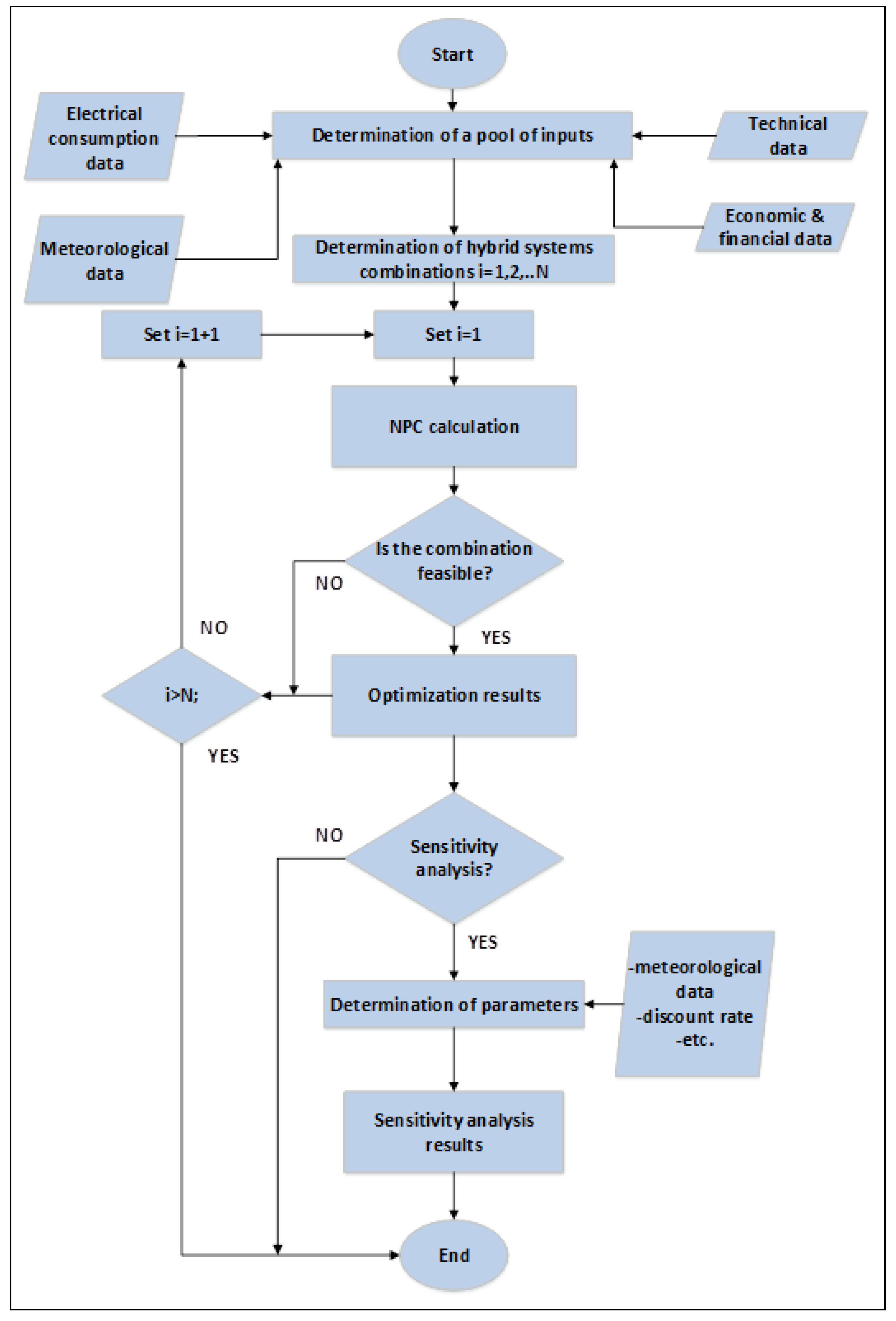
Figure 1.
Flow-chart of the methodology.
Figure 1.
Flow-chart of the methodology.
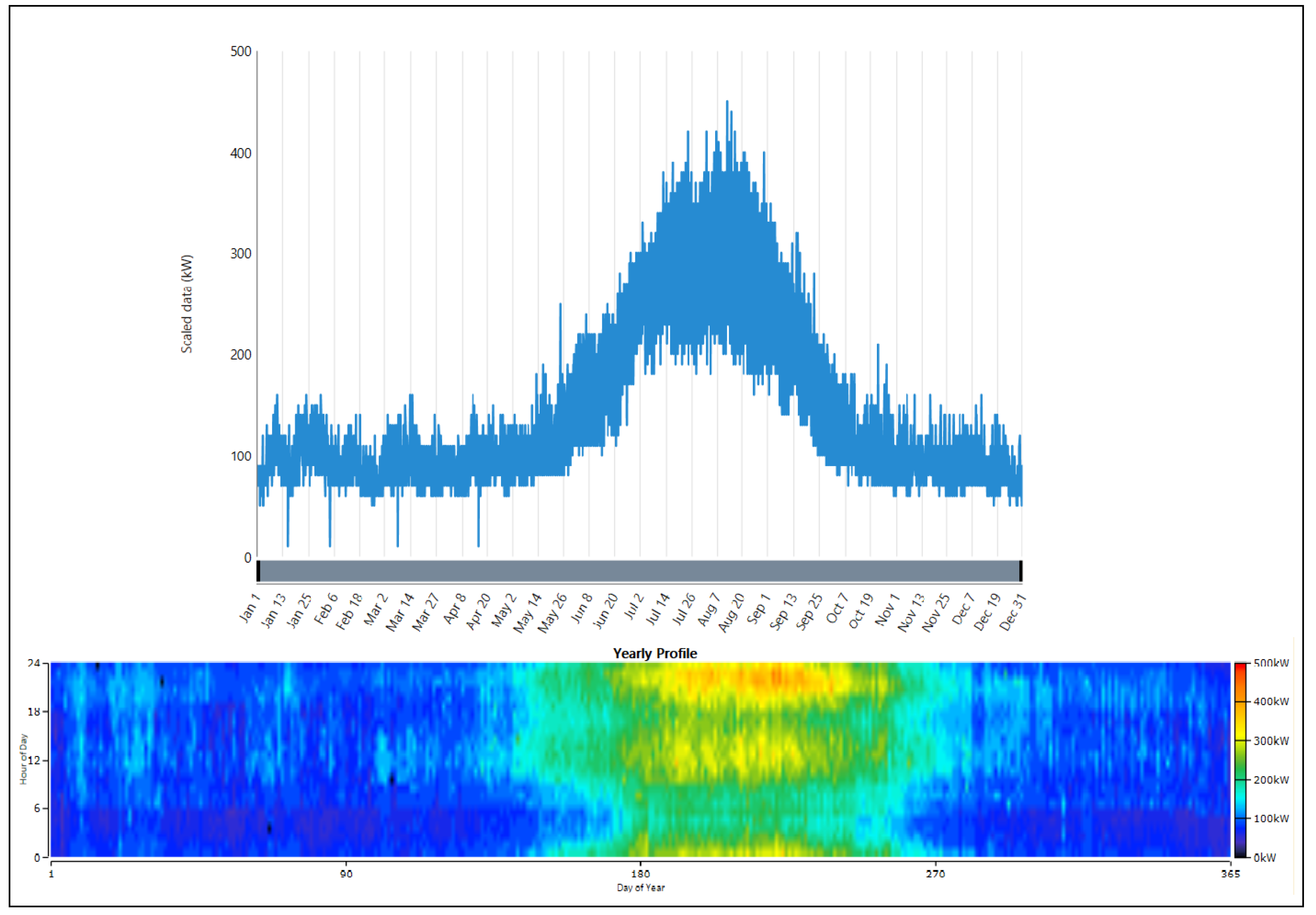
Figure 2.
Annual load of Donoussa and Data-Map of the monthly load profile.
Figure 2.
Annual load of Donoussa and Data-Map of the monthly load profile.
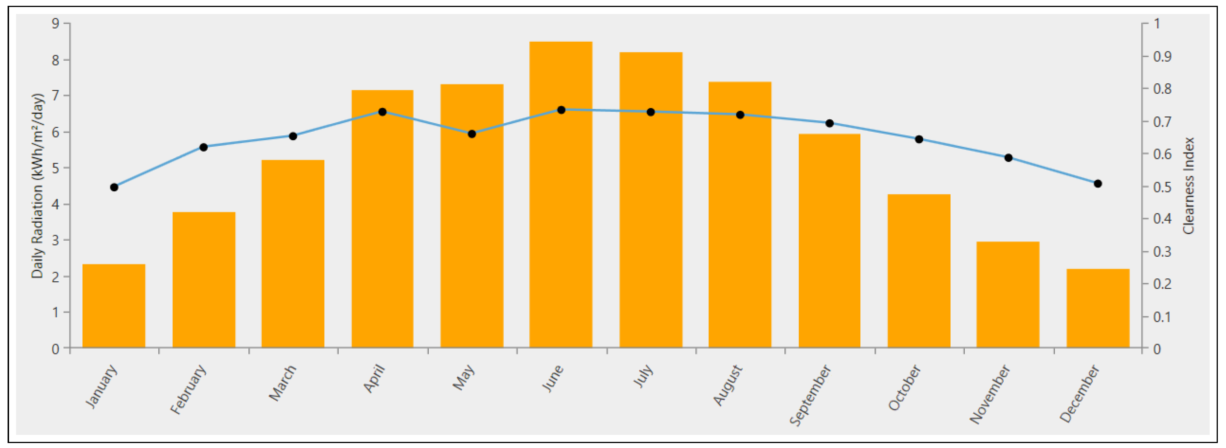
Figure 3.
Monthly Solar Radiation Sources and Clearness Index.
Figure 3.
Monthly Solar Radiation Sources and Clearness Index.
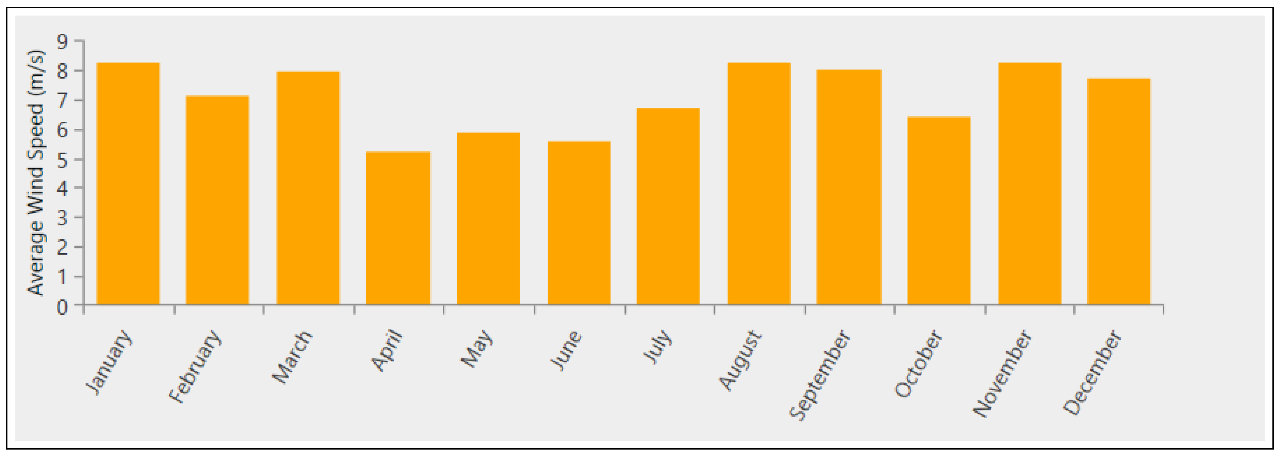
Figure 4.
Average monthly wind speed of Donoussa island.
Figure 4.
Average monthly wind speed of Donoussa island.
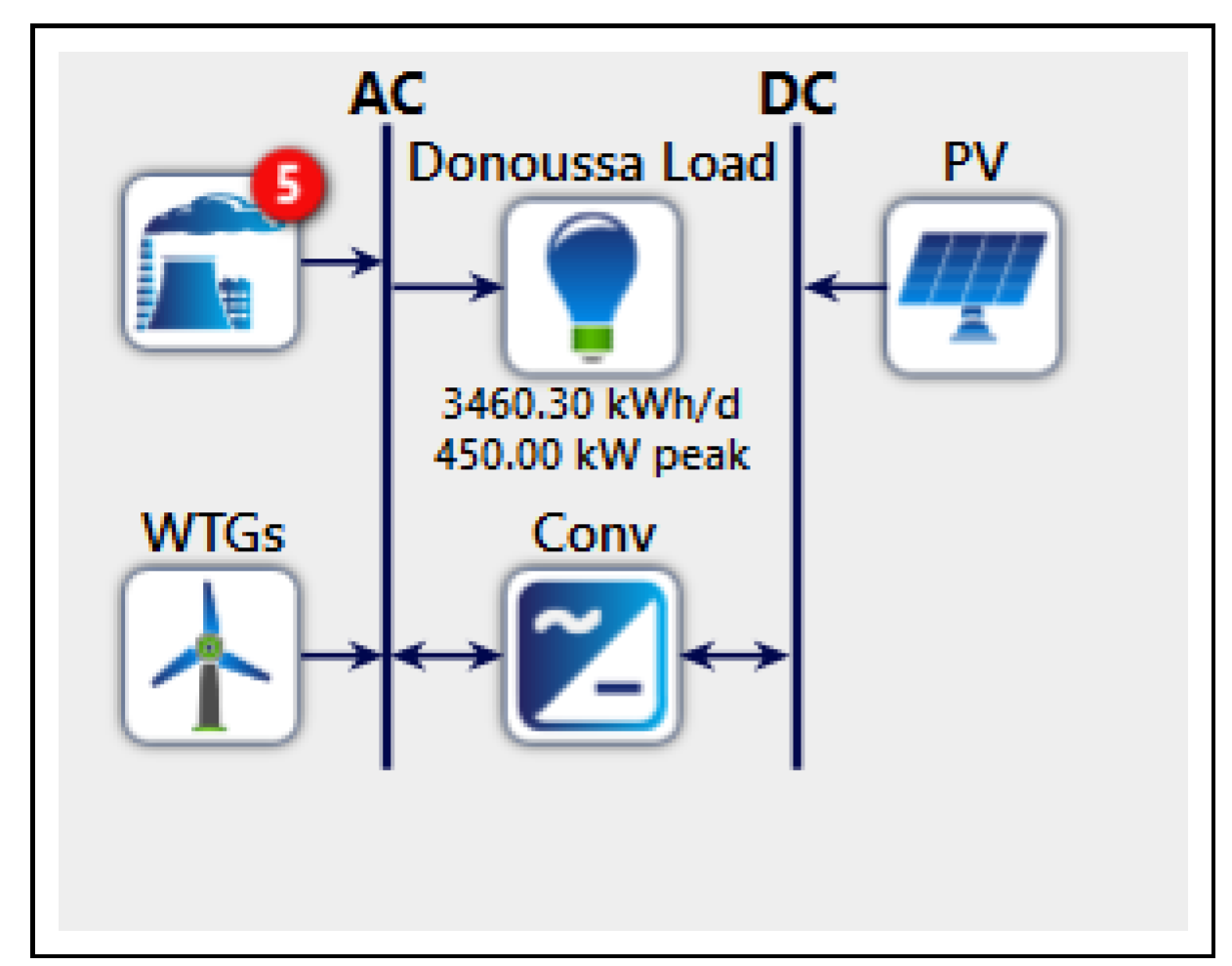
Figure 5.
Scenario 1 Homer Pro Configuration.
Figure 5.
Scenario 1 Homer Pro Configuration.
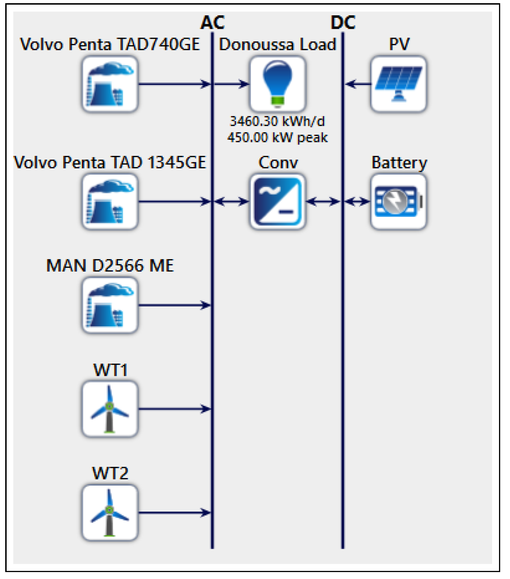
Figure 6.
Scenario 2 Homer Pro Configuration.
Figure 6.
Scenario 2 Homer Pro Configuration.
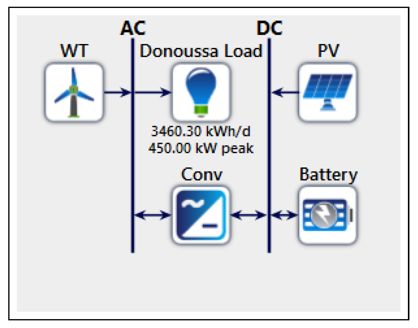
Figure 7.
Scenario 3 Homer Pro Configuration.
Figure 7.
Scenario 3 Homer Pro Configuration.
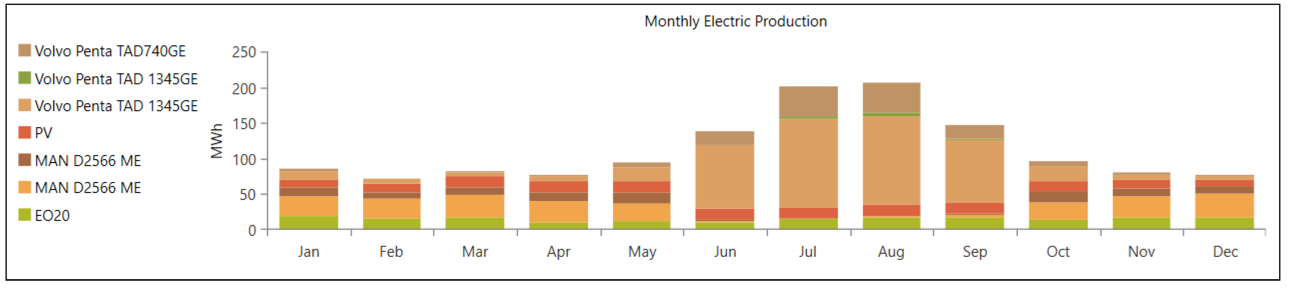
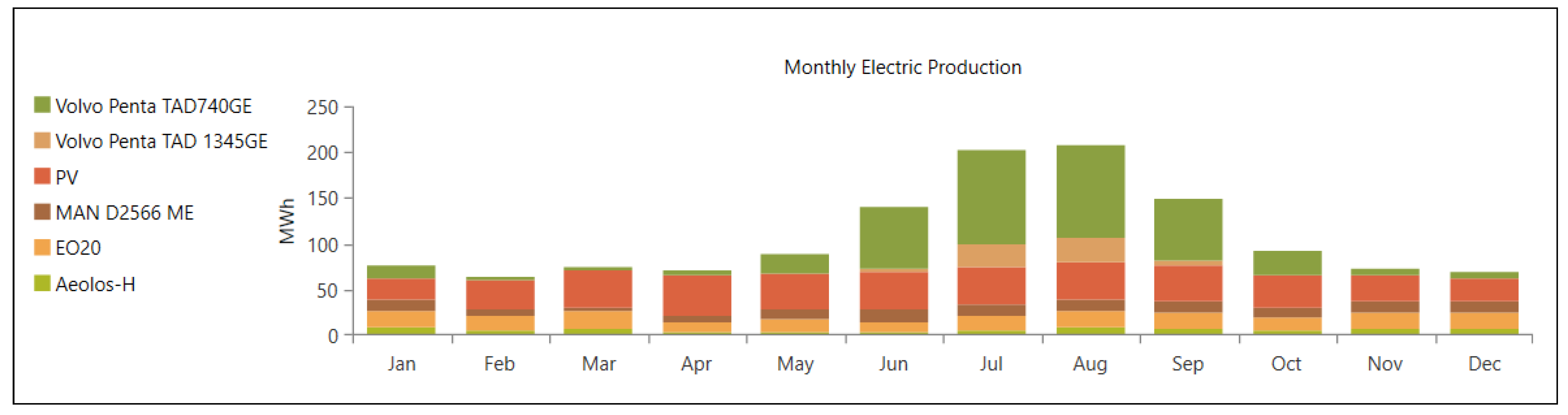
Figure 8.
Monthly Electrical Production of Scenario 1.
Figure 8.
Monthly Electrical Production of Scenario 1.
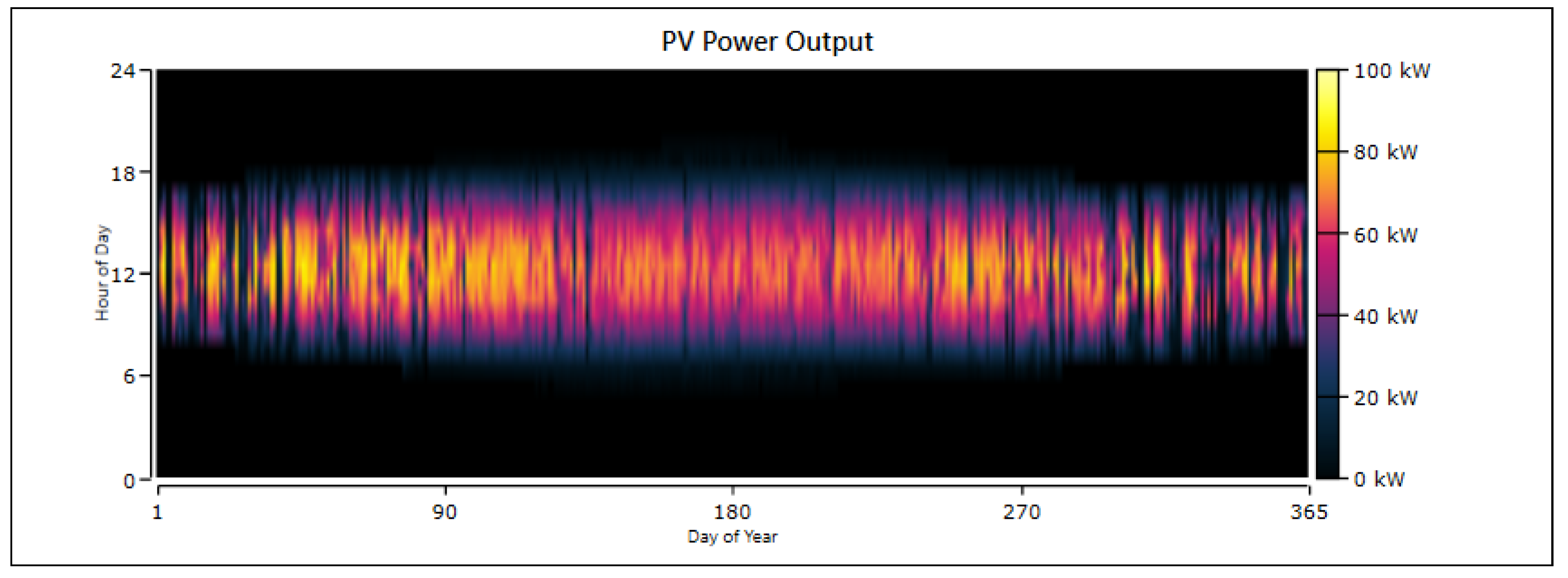
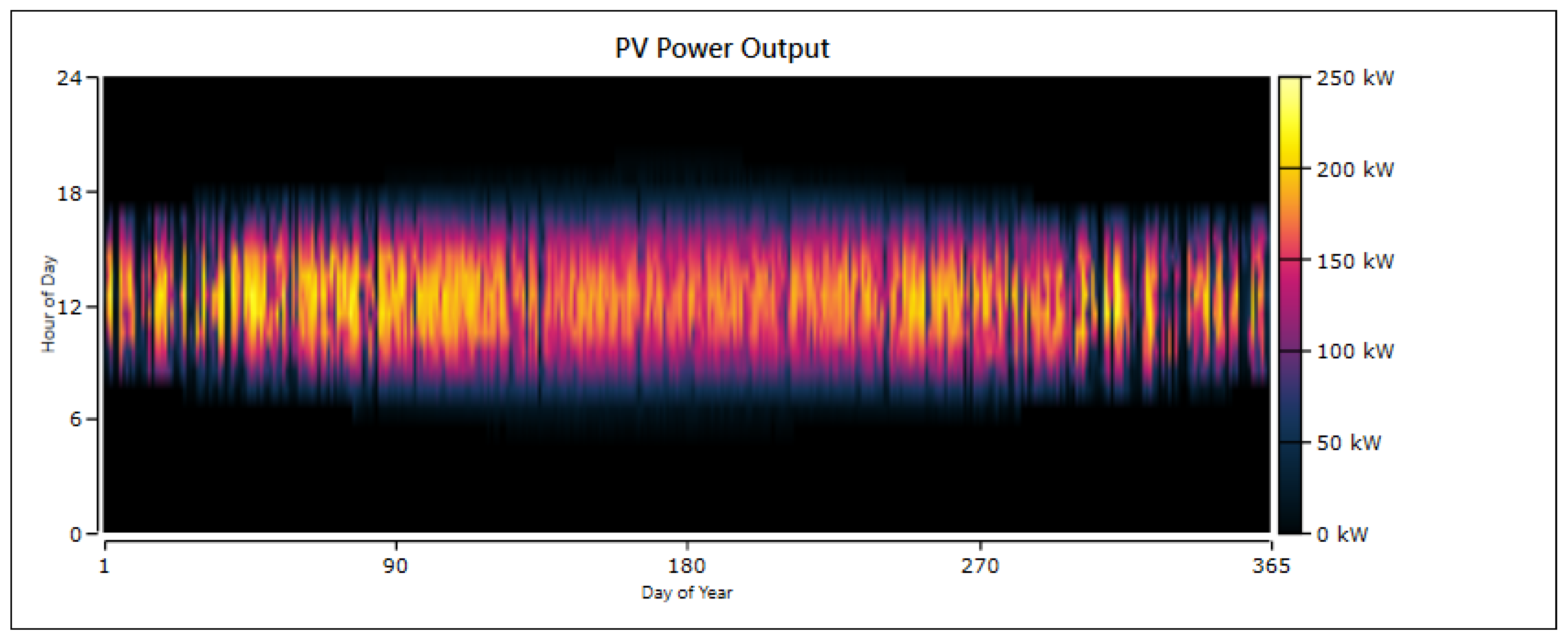
Figure 9.
PV Power output.
Figure 9.
PV Power output.
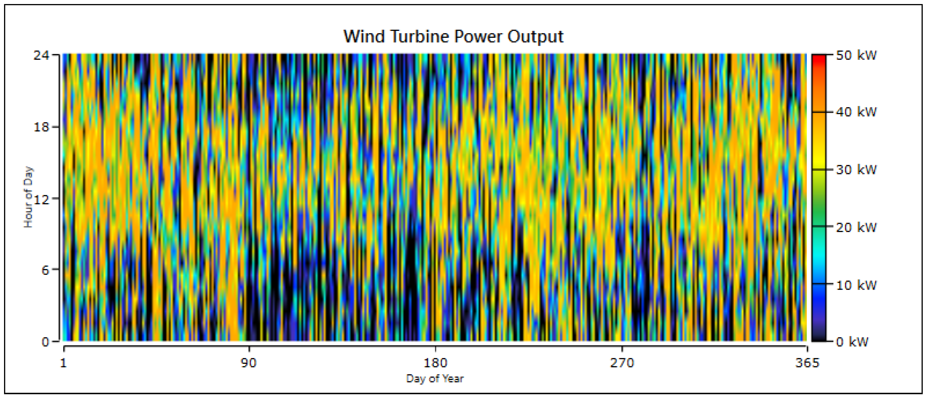
Figure 10.
Wind Turbine Power output.
Figure 10.
Wind Turbine Power output.
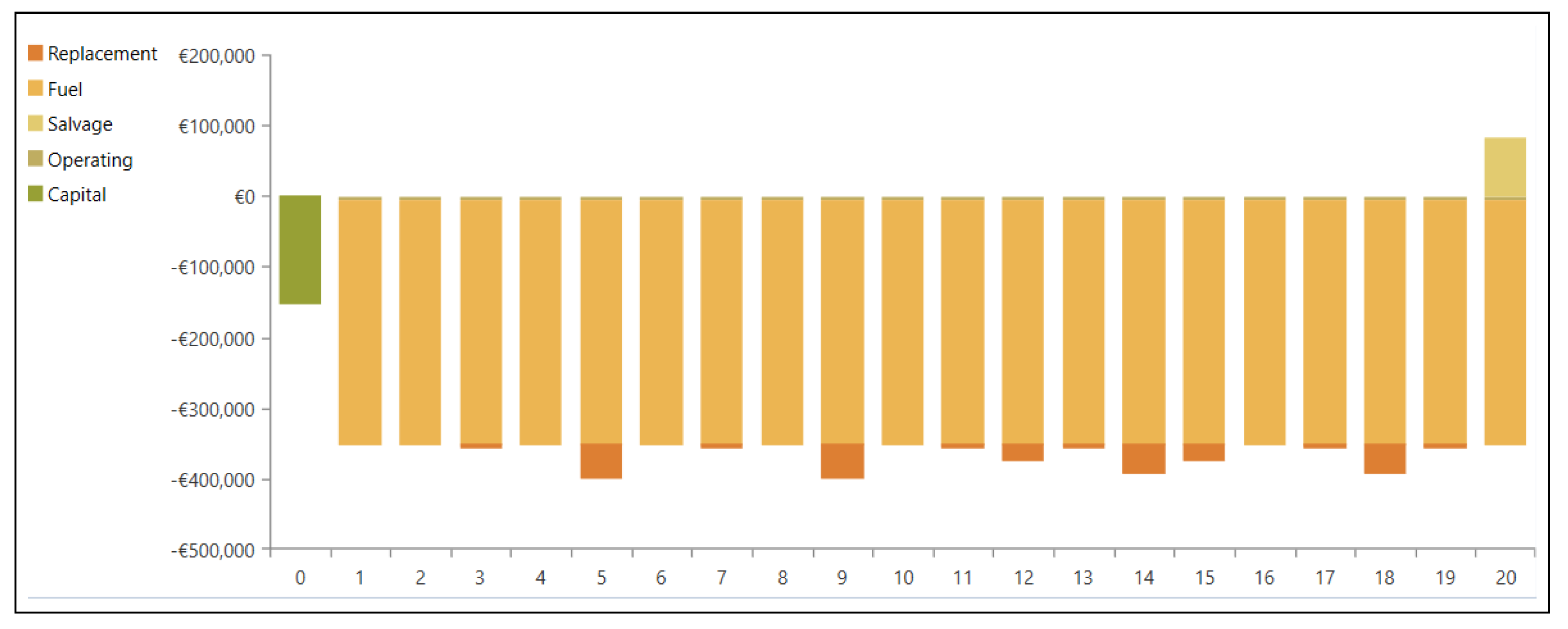
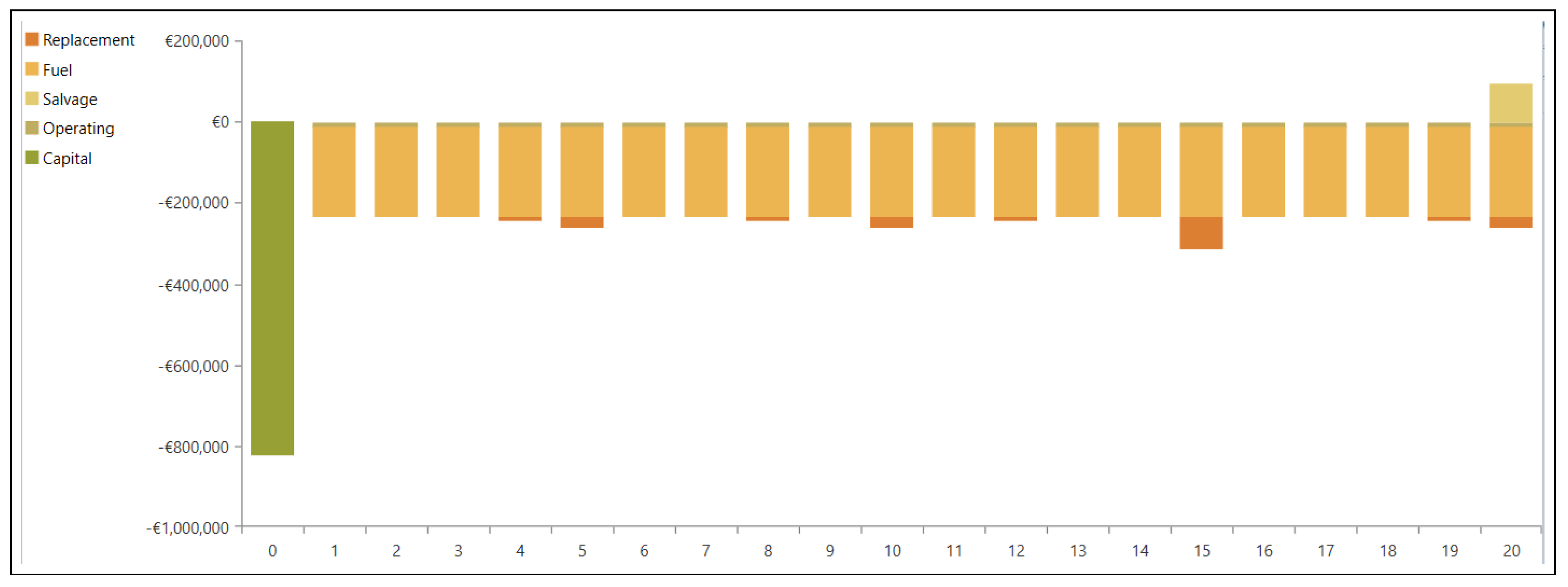
Figure 11.
Cash flow by Cost type Scenario 1.
Figure 11.
Cash flow by Cost type Scenario 1.
Figure 12.
Monthly electrical production of each component of Scenario 2.
Figure 12.
Monthly electrical production of each component of Scenario 2.
Figure 13.
PV power output Scenario 2.
Figure 13.
PV power output Scenario 2.
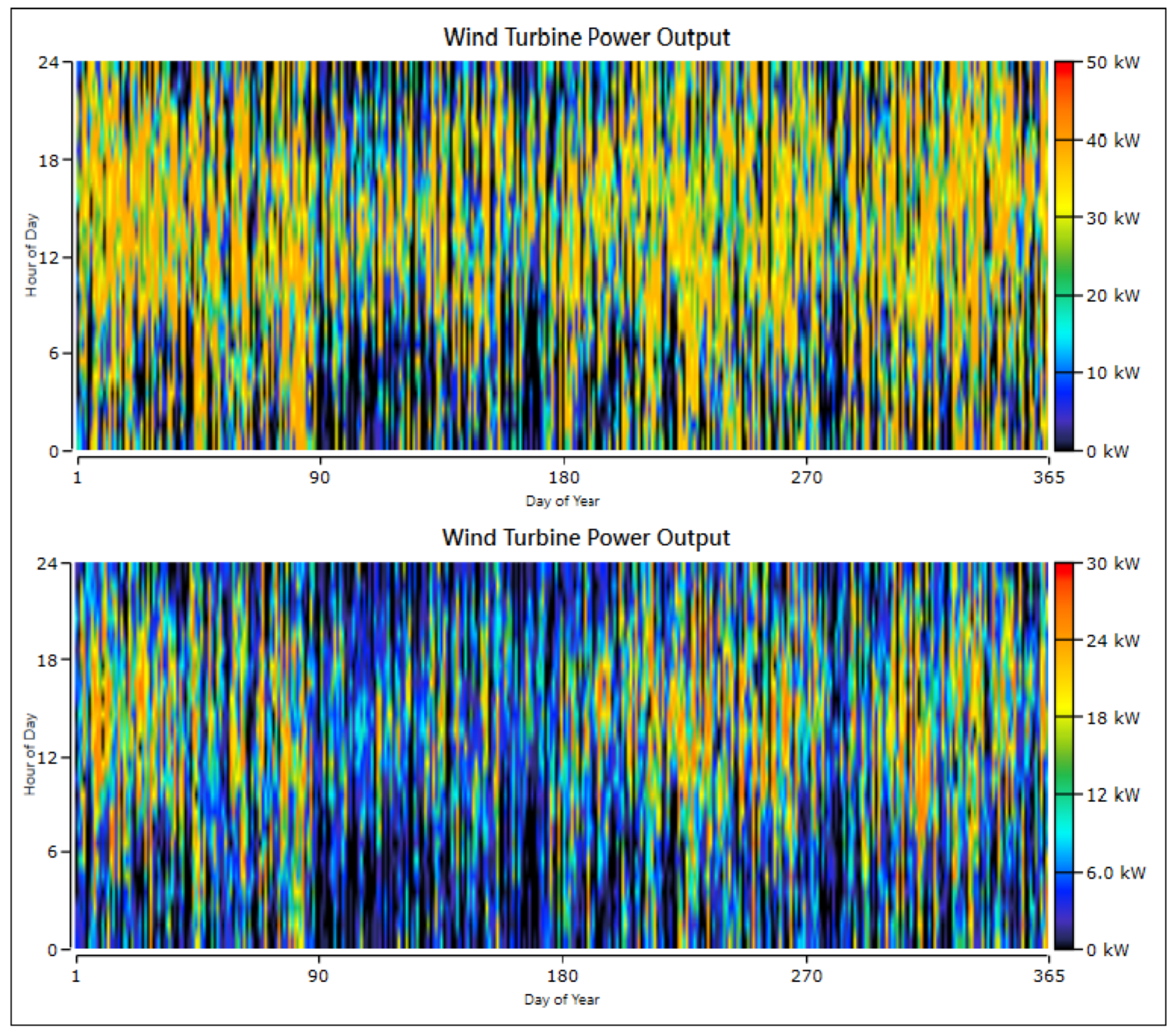
Figure 14.
Eocycle EO20 (20 kW) (upper figure) and Aeolos-H (10 kW) (down figure) power output Scenario 2.
Figure 14.
Eocycle EO20 (20 kW) (upper figure) and Aeolos-H (10 kW) (down figure) power output Scenario 2.
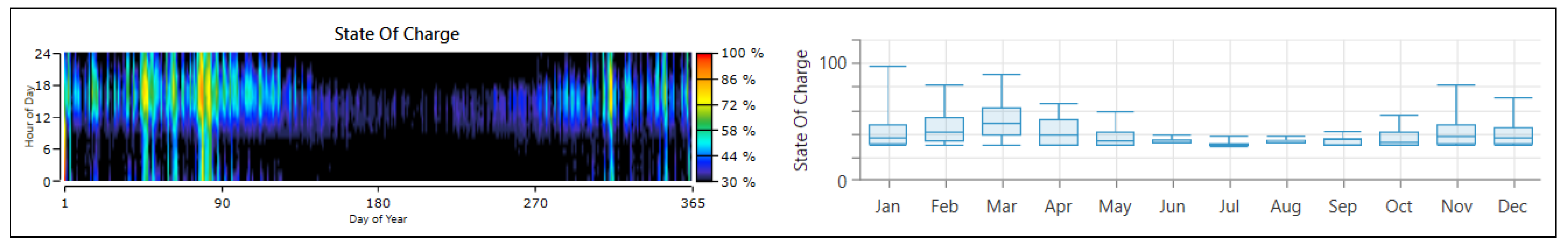
Figure 15.
Battery State-of-Charge Scenario 2.
Figure 15.
Battery State-of-Charge Scenario 2.
Figure 16.
Cash flow by Cost Type Scenario 2.
Figure 16.
Cash flow by Cost Type Scenario 2.
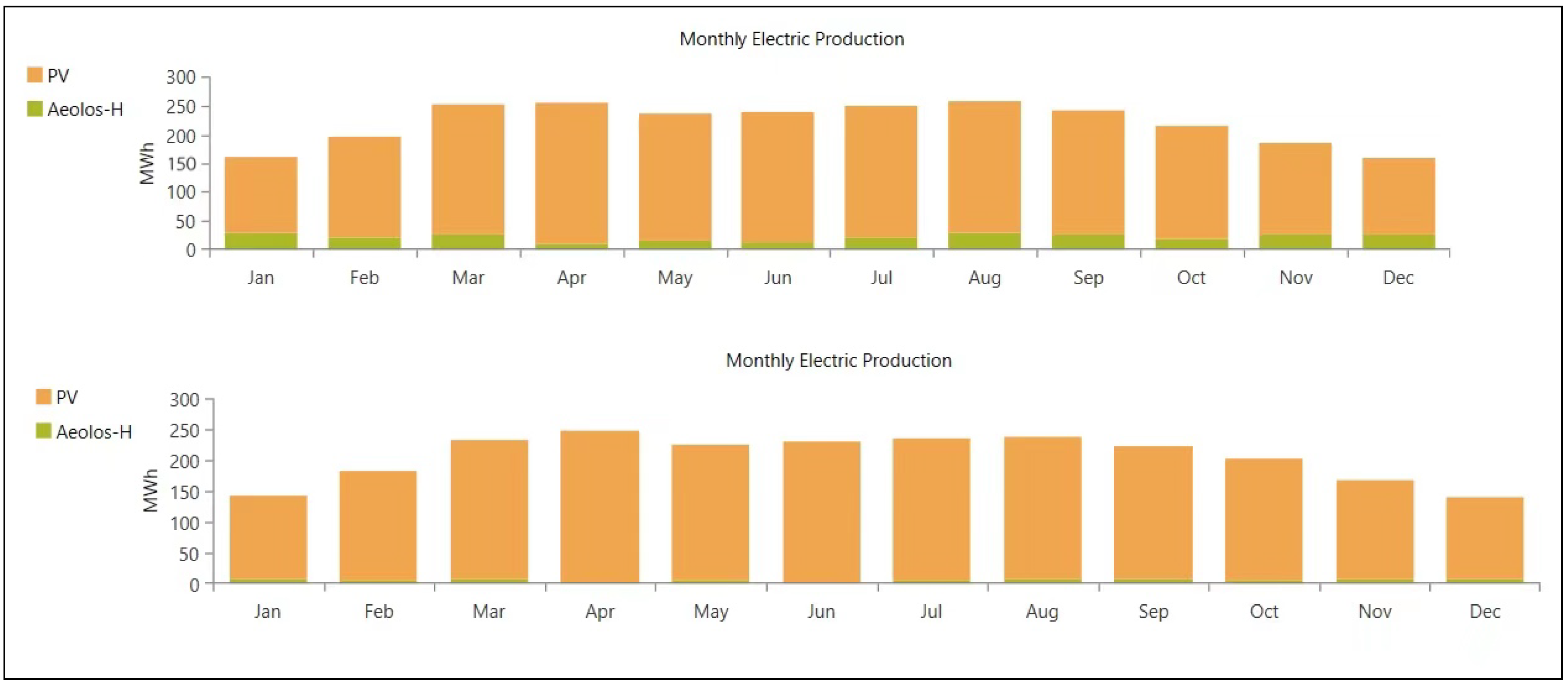
Figure 17.
Monthly electrical Production Case 1 (upper figure) and Case 2 (bottom figure) Scenario 3.
Figure 17.
Monthly electrical Production Case 1 (upper figure) and Case 2 (bottom figure) Scenario 3.
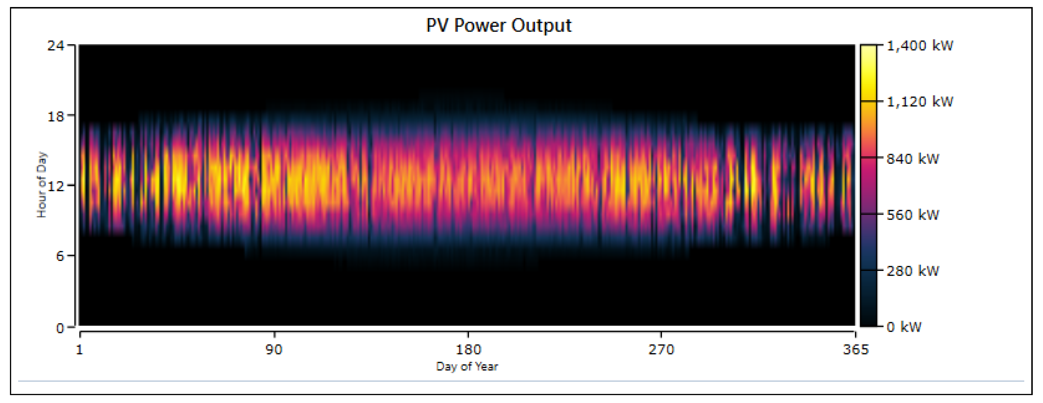
Figure 18.
PV power output Case 1 and Case 2 Scenario 3.
Figure 18.
PV power output Case 1 and Case 2 Scenario 3.
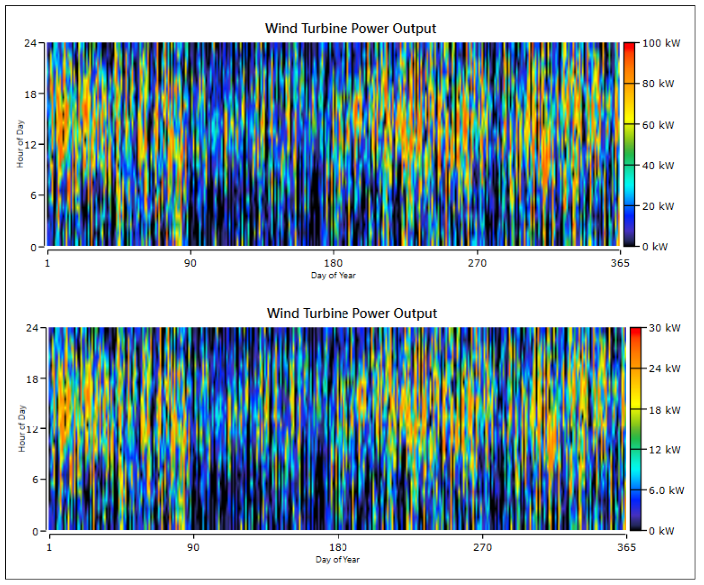
Figure 19.
Wind power output Case 1 (upper figure) and Case2 (bottom figure) Scenario 3.
Figure 19.
Wind power output Case 1 (upper figure) and Case2 (bottom figure) Scenario 3.
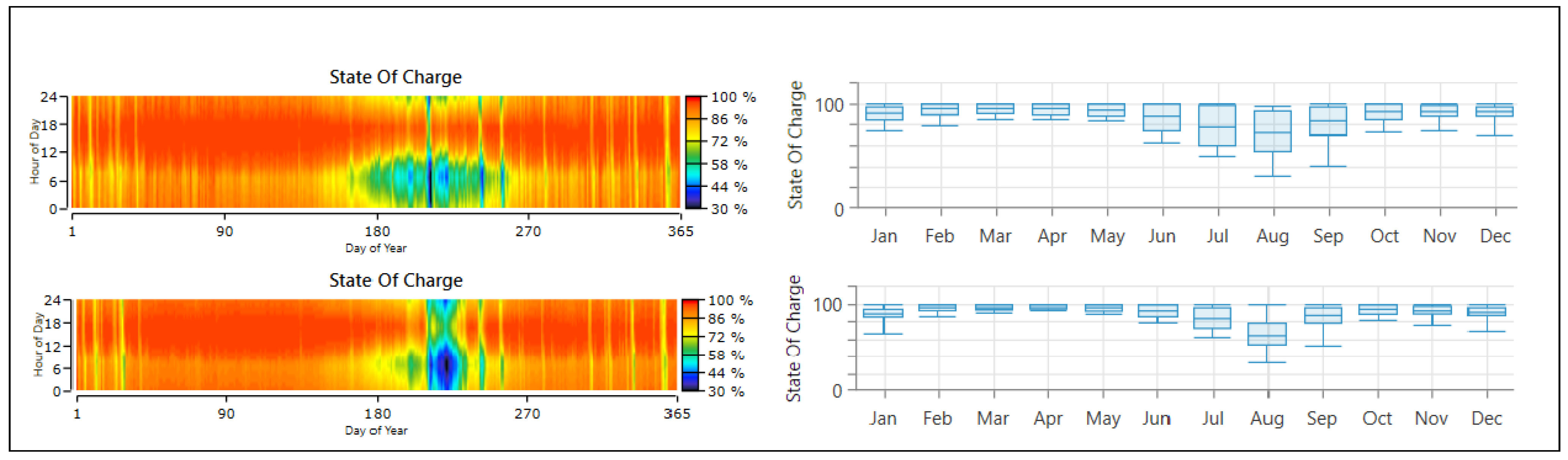
Figure 20.
Battery State-of-Charge Case 1 (upper) and Case 2 (bottom) Scenario 3.
Figure 20.
Battery State-of-Charge Case 1 (upper) and Case 2 (bottom) Scenario 3.
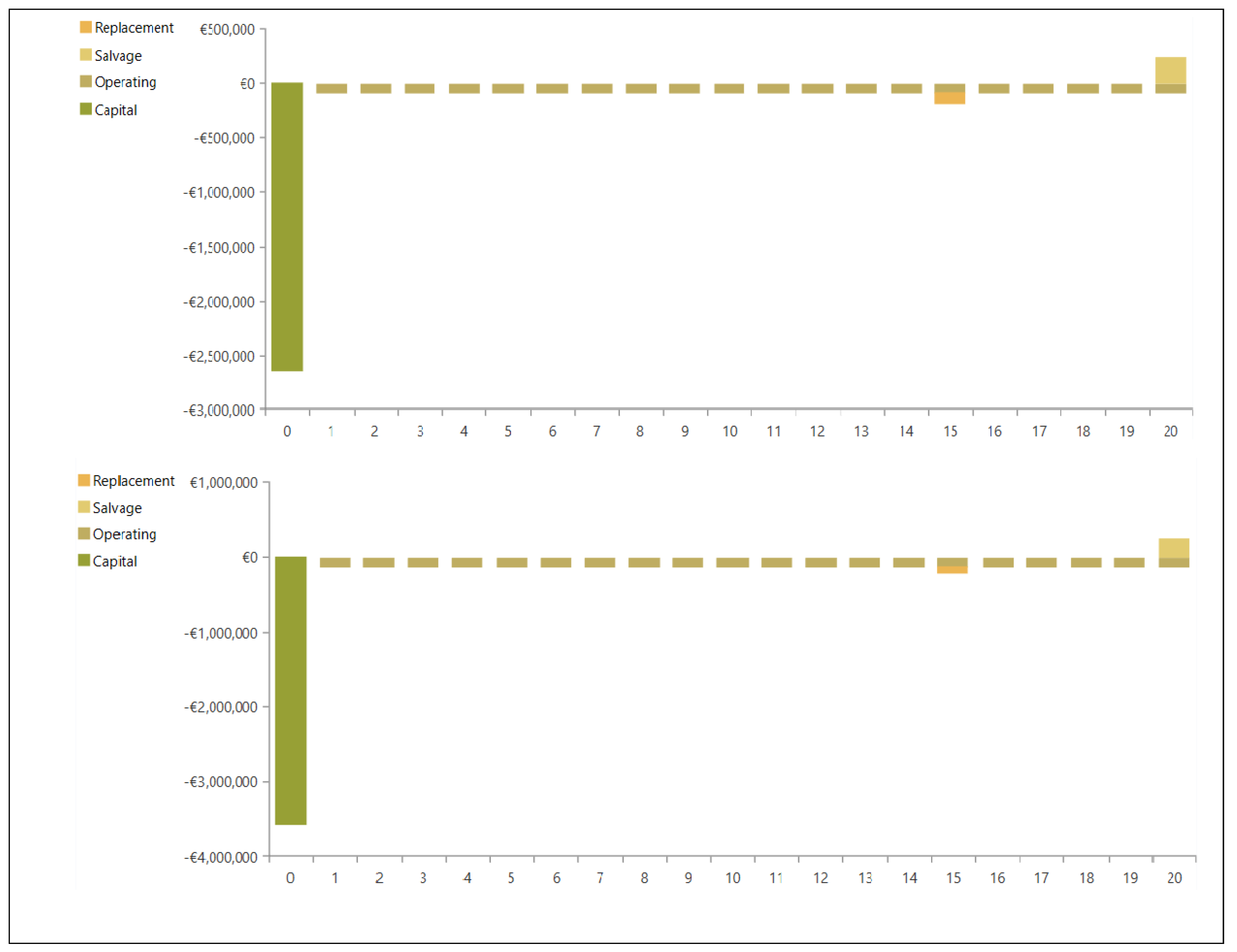
Figure 21.
Cash flow summary by Cost Type Case 1 (upper) and Case 2 (bottom) Scenario 3.
Figure 21.
Cash flow summary by Cost Type Case 1 (upper) and Case 2 (bottom) Scenario 3.
Table 1.
Types of generators and their characteristics of Donoussa thermal plant provided by HEDNO [
32].
Table 1.
Types of generators and their characteristics of Donoussa thermal plant provided by HEDNO [
32].
| No. | Type of Generator | Fuel | P (MW) | P (MW) |
|---|
| 1 | MAN D2566ME | DIESEL | 0.080 | 0.045 |
| 2 | MAN D2566ME | DIESEL | 0.080 | 0.045 |
| 3 | MAN D2566ME | DIESEL | 0.080 | 0.045 |
| 4 | VOLVO PENTA TAD 1345GE | DIESEL | 0.250 | 0.100 |
| 5 | VOLVO PENTA TAD 1345GE | DIESEL | 0.250 | 0.100 |
| 6 | VOLVO PENTA TAD 740GE | DIESEL | 0.200 | 0.110 |
Table 2.
Donoussa monthly average solar radiation data.
Table 2.
Donoussa monthly average solar radiation data.
| Month | Clearness Index | Daily Radiation kWh/m/day |
|---|
| January | 0.494 | 2.339 |
| February | 0.617 | 3.759 |
| March | 0.651 | 5.194 |
| April | 0.726 | 7.133 |
| May | 0.658 | 7.290 |
| June | 0.732 | 8.467 |
| July | 0.725 | 8.194 |
| August | 0.717 | 7.355 |
| September | 0.691 | 5.933 |
| October | 0.642 | 4.258 |
| November | 0.585 | 2.940 |
| December | 0.506 | 2.181 |
Table 3.
Donoussa monthly average wind speed data.
Table 3.
Donoussa monthly average wind speed data.
| Month | Average Wind Speed (m/s) |
|---|
| January | 8.250 |
| February | 7.080 |
| March | 7.950 |
| April | 5.200 |
| May | 5.880 |
| June | 5.560 |
| July | 6.680 |
| August | 8.250 |
| September | 8.000 |
| October | 6.380 |
| November | 8.250 |
| December | 7.720 |
Table 4.
PV technical speciifications and costs.
Table 4.
PV technical speciifications and costs.
| Parameters (Units) | Value |
|---|
| Panel type | Flat plate |
| Derating factor (%) | 80% |
| Operating temperature (C) | 47 C |
| Temperature coefficient | −0.5 |
| Ground reflection (%) | 20% |
| Lifetime (years) | 25 years |
| Tracking system | No Tracking System |
| Capital Cost (€) | 620 €/kW |
| Replacement Cost (€) | 620 €/kW |
| Operation and Maintenance Cost (€/year) | 14 €/year |
| Search Space Scenario 1 | 40, 50, 60, 70, 80, 90, 100 kW |
| Search Space Scenario 2 | 180, 190, 200, 210, 220, 230, 240, 250, 260 kW |
| Search Space Scenario 3 Case 1 | 1200, 1250, 1300, 1350, 1400, 1450, 1500, 1550 kW |
| Search Space Scenario 3 Case 2 | 1400, 1450, 1500, 1550, 1600, 1650, 1700, 1750 kW |
Table 5.
Technical specifications and Costs of Eocycle EO20 Wind Turbine.
Table 5.
Technical specifications and Costs of Eocycle EO20 Wind Turbine.
| Parameters (Units) | Value |
|---|
| Model | Eocycle EO20 |
| Nominal Capacity (kW) | 20 kW |
| Rotor Diameter (m) | 15.8 m |
| Cut-in/out wind speed (m/s) | 2.75 m/s–20.00 m/s |
| Hub/tower height (m) | 36 m |
| Capital Cost (€) | 35,800 € |
| Replacement Cost (€) | 28,640 € |
| Operation and Maintenance Cost (/year) | 1075 €/year |
| Scenario 1 Search Space | 1, 2 units |
| Scenario 2 Search Space | 1, 2 units |
Table 6.
Technical specifications and Costs of Aeolos-H 10 kW Wind Turbine.
Table 6.
Technical specifications and Costs of Aeolos-H 10 kW Wind Turbine.
| Parameters (Units) | Value |
|---|
| Model | Aeolos-H 10 kW |
| Nominal Capacity (kW) | 10 kW |
| Rotor Diameter (m) | 8 m |
| Cut-in/out wind speed (m/s) | 3 m/s–10.00 m/s |
| Hub/tower height (m) | 24 m |
| Capital Cost (€) | 17,900 € |
| Replacement Cost (€) | 14,320 € |
| Operation and Maintenance Cost (€/year) | 540 €/year |
| Scenario 2 Search Space | 1, 2 units |
| Scenario 3 Search Space Case 1 | 1, 2, 3, 4, 5, 6, 7 units |
| Scenario 3 Search Space Case 2 | 1, 2 units |
Table 7.
Technical specifications and costs of Hoppecke 24 OPzS 3000 battery.
Table 7.
Technical specifications and costs of Hoppecke 24 OPzS 3000 battery.
| Parameters (Units) | Value |
|---|
| Nominal Voltage (V) | 2 V |
| Nominal Capacity (kWh) | 7.15 kWh |
| Maximum Capacity (Ah) | 3570 Ah |
| Round efficiency (%) | 86% |
| Minimum State of Charge (%) | 30% |
| Maximum Charge Current (A) | 610 A |
| Lifetime (years) | 20 years |
| Capital Cost (€) | 1200 € |
| Replacement Cost (€) | 840 € |
| Operating and Maintenance Cost (€/year) | 12 €/year |
Table 8.
Scenario 1 Optimization results.
Table 8.
Scenario 1 Optimization results.
| Systems | PV (kW) | EO20 (WT) | TAD 740GE (kW) | TAD 1345GE (kW) | TAD 1345GE (kW) | D2566 ME (kW) | D2566 ME (kW) | Conv (kW) | Excess Elec (%) | NPC (Millions €) | COE (€) | Ren Frac (%) | Dispatch |
|---|
| System 1 | 100 | 2 | 200 | 250 | 250 | 80 | 80 | 80 | 6.68 | 4.95 | 0.295 | 20.2 | CC |
Table 9.
Analytical Electrical Production and technical characteristics for optimal configuration of Scenario 1.
Table 9.
Analytical Electrical Production and technical characteristics for optimal configuration of Scenario 1.
| System Components | Production (kWh/year) | Production % | Mean Output (kW) | Annual Fuel Consumption L/year | Operational Hours h/year |
|---|
| PV | 164,853 | 12.1 | 18.8 | - | 4386 |
| TAD740GE | 151,860 | 11.2 | 112 | 36,447 | 1353 |
| TAD 1345GE | 509,656 | 37.5 | 150 | 119,781 | 3396 |
| TAD 1345GE | 9486 | 0.698 | 112 | 2,229 | 85 |
| MAN D2566 ME | 234,188 | 17.2 | 45 | 27,737 | 2291 |
| MAN D2566 ME | 103,095 | 7.59 | 47.1 | 63,022 | 4976 |
| Eocycle EO20 | 185,982 | 13.7 | 21.2 | - | 7708 |
| Total | 1,359,120 | 100 | - | 249,215 | - |
Table 10.
PV Scheme Simulation Results.
Table 10.
PV Scheme Simulation Results.
| Quantity | Value | Units |
|---|
| Rated capacity | 100 | kW |
| Minimum Output | 0 | kW |
| Maximum Output | 88.6 | kW |
| Mean Output | 18.8 | kW |
| Mean Output | 452 | kWh/d |
| Capacity Factor | 18.8 | % |
| Total Production | 164,853 | kWh/year |
| PV Penetration | 13.1 | % |
| Hours of Operation | 4386 | h/year |
| Levelized Cost | 0.0343 | €/kWh |
Table 11.
Wind Turbines Scheme Simulation Results.
Table 11.
Wind Turbines Scheme Simulation Results.
| Quantity | Value | Units |
|---|
| Rated capacity | 20 | kW |
| Minimum Output | 0 | kW |
| Maximum Output | 40.6 | kW |
| Mean Output | 21.2 | kW |
| Capacity Factor | 53.1 | % |
| Total Production | 185,982 | kWh/year |
| Wind Penetration | 14.7 | % |
| Hours of Operation | 7708 | hrs/year |
| Levelized Cost | 0.0405 | €/kWh |
Table 12.
Economic characteristics of the optimal configuration of Scenario 1.
Table 12.
Economic characteristics of the optimal configuration of Scenario 1.
| System | NPC (€) | LCoE (€) | Capital (€) | Replacement (€) | Salvage (€) | O & M (€/year) | Fuel (€) |
|---|
| Optimal | 4,950,407.61 | 0.2948 | 153,600 | 175,581.04 | −36,535.63 | 62,424.89 | 4,595,337.32 |
Table 13.
Analytical costs of each component Scenario 1.
Table 13.
Analytical costs of each component Scenario 1.
| Component | Capital (€) | Replacement (€) | O & M (€) | Fuel (€) | Salvage (€) | Total (€) |
|---|
| Eocycle E020 | 71,600 | 0.00 | 28,556.30 | 0.00 | 0.00 | 100,156.30 |
| Generic Flat plate PV | 62,000 | 0.00 | 18,612.11 | 0.00 | −5393.87 | 75,218.24 |
| Generic large, free converter | 20,000 | 9855.46 | 0.00 | 0.00 | −5335.87 | 24,519.59 |
| MAN D2566 ME | 0.00 | 36,378.24 | 3969.17 | 1,162,073.04 | −125.28 | 1,202,295.17 |
| MAN D2566 ME | 0.00 | 15,555.28 | 1827.44 | 511,442.71 | −1090.95 | 527,734.48 |
| VOLVO PENTA TAD1345GE | 0.00 | 98,032.64 | 6772.15 | 2,208,667.27 | −7801.97 | 2,305,670.09 |
| VOLVO PENTA TAD1345GE | 0.00 | 0.00 | 169.50 | 41,106.68 | −14,656.24 | 26,619.94 |
| VOLVO PENTA TAD1740GE | 0.00 | 15,759.42 | 2518.22 | 672,047.62 | −2131.45 | 688,193.81 |
| System | 153,600 | 175,581.04 | 62,424.89 | 4,595,337.32 | −36,535.63 | 4,950,407.61 |
Table 14.
Scenario 2 Optimization results.
Table 14.
Scenario 2 Optimization results.
| Systems | PV (kW) | EO20 (WT) | Aeolos-H | TAD 740GE (kW) | TAD 1345GE (kW) | D2566 ME (kW) | Battery | Conv (kW) | Excess Elec (%) | NPC (Millions €) | COE (€) | Ren Frac (%) | Dispatch |
|---|
| System 1 | 260 | 2 | 2 | 200 | 250 | 80 | 420 | 200 | 0 | 4.03 | 0.240 | 51.0 | LF |
Table 15.
Analytical electrical Production and technical characteristics for optimal configuration of Scenario 2.
Table 15.
Analytical electrical Production and technical characteristics for optimal configuration of Scenario 2.
| System Components | Production (kWh/year) | Production % | Mean Output (kW) | Annual Fuel Consumption (L/year) | Operational Hours (h/year) |
|---|
| PV | 428,618 | 32.8 | 48.9 | - | 4386 |
| TAD740GE | 429,150 | 32.8 | 136 | 109,093 | 3153 |
| TAD 1345GE | 60,600 | 4.63 | 111 | 17,332 | 548 |
| MAN D2566 ME | 128,867 | 9.85 | 47.7 | 34,682 | 2703 |
| Eocycle EO20 | 185,982 | 14.2 | 21.2 | - | 7708 |
| Aeolos-H (10 kW) | 74,579 | 5.70 | 8.51 | - | 7374 |
| Total | 1,307,797 | 100 | - | 161,106 | - |
Table 16.
PV Scheme Simulation Results.
Table 16.
PV Scheme Simulation Results.
| Quantity | Value | Units |
|---|
| Rated capacity | 260 | kW |
| Minimum Output | 0 | kW |
| Maximum Output | 230 | kW |
| Mean Output | 48.9 | kW |
| Mean Output | 1174 | kWh/d |
| Capacity Factor | 18.8 | % |
| Total Production | 428,618 | kWh/year |
| PV Penetration | 33.9 | % |
| Hours of Operation | 4386 | h/year |
| Levelized Cost | 0.0343 | €/kWh |
Table 17.
Eocycle EO20 (20 kW) Scheme Simulation Results.
Table 17.
Eocycle EO20 (20 kW) Scheme Simulation Results.
| Quantity | Value | Units |
|---|
| Rated capacity | 40 | kW |
| Minimum Output | 0 | kW |
| Maximum Output | 40.6 | kW |
| Mean Output | 21.2 | kW |
| Capacity Factor | 53.1 | % |
| Total Production | 185,982 | kWh/year |
| Wind Penetration | 14.7 | % |
| Hours of Operation | 7708 | h/year |
| Levelized Cost | 0.0405 | €/kWh |
Table 18.
Aeolos-H (10 kW) Scheme Simulation Results.
Table 18.
Aeolos-H (10 kW) Scheme Simulation Results.
| Quantity | Value | Units |
|---|
| Rated capacity | 20 | kW |
| Minimum Output | 0 | kW |
| Maximum Output | 27.6 | kW |
| Mean Output | 8.51 | kW |
| Capacity Factor | 42.6 | % |
| Total Production | 74,579 | kWh/year |
| Wind Penetration | 5.9 | % |
| Hours of Operation | 7374 | h/year |
| Levelized Cost | 0.0506 | €/kWh |
Table 19.
Battery Scheme Simulation Results.
Table 19.
Battery Scheme Simulation Results.
| Quantity | Value | Units |
|---|
| Batteries | 420 | qty |
| String Size | 12.0 | batteries |
| Strings in Parallel | 35.0 | strings |
| Bus Voltage | 24.0 | V |
| Autonomy | 14.6 | hr |
| Storage Wear Cost | 0.0895 | €/kWh |
| Nominal Capacity | 3003 | kWh |
| Usable Nominal Capacity | 2102 | kWh |
| Energy In | 162,376 | kWh/year |
| Energy Out | 141,538 | kWh/year |
| Storage Depletion | 2043 | kWh/year |
| Losses | 22,881 | kWh/year |
| Annual Throughput | 152,625 | kWh/year |
Table 20.
Economic characteristics of the optimal configuration of Scenario 2.
Table 20.
Economic characteristics of the optimal configuration of Scenario 2.
| System | NPC (€) | LCoE (€) | Capital (€) | Replacement (€) | Salvage (€) | O & M (€/year) | Fuel (€) |
|---|
| Optimal | 4,031,102 | 0.2401 | 822,600 | 112,901.73 | −42,539.07 | 167,453.17 | 2,970,686.19 |
Table 21.
Analytical costs of each component Scenario 2.
Table 21.
Analytical costs of each component Scenario 2.
| Component | Capital (€) | Replacement (€) | O & M (€) | Fuel (€) | Salvage (€) | Total (€) |
|---|
| Aeolos-H 10 kW | 35,800.00 | 0.00 | 14,357.92 | 0.00 | 0.00 | 50,157.92 |
| Eocycle EO20 | 71,600.00 | 0.00 | 25,582.89 | 0.00 | 0.00 | 100,182.89 |
| Generic Flat plate PV | 161,200.00 | 0.00 | 48,391.49 | 0.00 | −14,024.06 | 195,567.43 |
| Generic large, free converter | 50,000.00 | 24,638.65 | 0.00 | 0.00 | −13,339.68 | 61,298.97 |
| Hoppecke 24OPzS 3000 | 504,000.00 | 0.00 | 67,003.60 | 0.00 | 0.00 | 571,003.60 |
| MAN D2566 ME | 0.00 | 25,803.75 | 2156.08 | 639,502.17 | −2067.07 | 665,394.93 |
| VOLVO PENTA TAD1345GE | 0.00 | 98,032.64 | 6772.15 | 2,208,667.27 | −7801.97 | 2,305,670.09 |
| VOLVO PENTA TAD1345GE | 0.00 | 0.00 | 1,092.80 | 319,589.11 | −4451.97 | 316,229.93 |
| VOLVO PENTA TAD740GE | 0.00 | 62,459.33 | 5868.40 | 2,011,594.91 | −8656.29 | 2,071,266.35 |
| System | 822,600.00 | 112,901.73 | 167,453.17 | 2,970,686.19 | −42,539.07 | 4,031,102.03 |
Table 22.
Analytical Electrical Production and technical characteristics for optimal configuration of Scenario 3 case 1.
Table 22.
Analytical Electrical Production and technical characteristics for optimal configuration of Scenario 3 case 1.
| System Components | Size | Electricity Production | Mean Output (kW) | Operational Hours (h/year) |
|---|
| kWh/year | % |
|---|
| PV | 1450 kW | 2,390,365 | 90.2 | 273 | 4386 |
| Aeolos-H (10 kW) | 7 (70 kW) | 261,025 | 9.84 | 29.8 | 7374 |
| Total | 1520 | 2,651,391 | 100 | - | - |
| Battery Hoppecke | 1260 (9009 kWh) | Energy in 678,208 kWh/year | Energy out 583,614 kWh/year | Annual throughput 629,327 kWh/year | Autonomy 43.7 h |
Table 23.
Analytical Electrical Production and technical characteristics for optimal configuration of Scenario 3 case 2.
Table 23.
Analytical Electrical Production and technical characteristics for optimal configuration of Scenario 3 case 2.
| System Components | Size | Electricity Production | Mean Output (kW) | Operational Hours (h/year) |
|---|
| kWh/year | % |
|---|
| PV | 1450 kW | 2,390,365 | 97 | 273 | 4386 |
| Aeolos-H (10 kW) | 2 (20 kW) | 74,579 | 3.03 | 8.51 | 7374 |
| Total | 1,470 | 2,464,944 | 100 | - | - |
| Battery Hoppecke | 2112 (15,099 kWh) | Energy in 783,923 kWh/year | Energy out 674,837 kWh/year | Annual throughput 727,696 kWh/year | Autonomy 73.3 h |
Table 24.
PV Scheme Simulation Results Case 1 and Case 2, Scenario 3.
Table 24.
PV Scheme Simulation Results Case 1 and Case 2, Scenario 3.
| Quantity | Value | Units |
|---|
| Rated capacity | 1450 | kW |
| Minimum Output | 0 | kW |
| Maximum Output | 1285 | kW |
| Mean Output | 273 | kW |
| Mean Output | 6549 | kWh/d |
| Capacity Factor | 18.8 | % |
| Total Production | 2,390,365 | kWh/year |
| PV Penetration | 189 | % |
| Hours of Operation | 4386 | h/year |
| Levelized Cost | 0.0343 | €/kWh |
Table 25.
Aeolos-H (10 kW) Scheme Simulation Results Case 1 Scenario 3.
Table 25.
Aeolos-H (10 kW) Scheme Simulation Results Case 1 Scenario 3.
| Quantity | Value | Units |
|---|
| Rated capacity | 70 | kW |
| Minimum Output | 0 | kW |
| Maximum Output | 96.6 | kW |
| Mean Output | 29.8 | kW |
| Capacity Factor | 42.6 | % |
| Total Production | 261,025 | kWh/year |
| Wind Penetration | 20.7 | % |
| Hours of Operation | 7374 | h/year |
| Levelized Cost | 0.0506 | €/kWh |
Table 26.
Aeolos-H (10 kW) Scheme Simulation Results Case 2 Scenario 3.
Table 26.
Aeolos-H (10 kW) Scheme Simulation Results Case 2 Scenario 3.
| Quantity | Value | Units |
|---|
| Rated capacity | 20 | kW |
| Minimum Output | 0 | kW |
| Maximum Output | 27.6 | kW |
| Mean Output | 8.51 | kW |
| Capacity Factor | 42.6 | % |
| Total Production | 74,579 | kWh/year |
| Wind Penetration | 5.90 | % |
| Hours of Operation | 7374 | h/year |
| Levelized Cost | 0.0506 | €/kWh |
Table 27.
Battery Scheme Simulation Results Case 1 Scenario 3.
Table 27.
Battery Scheme Simulation Results Case 1 Scenario 3.
| Quantity | Value | Units |
|---|
| Batteries | 1260 | qty |
| String Size | 12.0 | batteries |
| Strings in Parallel | 105 | strings |
| Bus Voltage | 24.0 | V |
| Autonomy | 43.7 | h |
| Storage Wear Cost | 0.0895 | €/kWh |
| Nominal Capacity | 9008 | kWh |
| Usable Nominal Capacity | 6306 | kWh |
| Energy In | 678,208 | kWh/year |
| Energy Out | 583,614 | kWh/year |
| Storage Depletion | 383 | kWh/year |
| Losses | 94,977 | kWh/year |
| Annual Throughput | 629,327 | kWh/year |
Table 28.
Battery Scheme Simulation Results Case 2 Scenario 3.
Table 28.
Battery Scheme Simulation Results Case 2 Scenario 3.
| Quantity | Value | Units |
|---|
| Batteries | 2112 | qty |
| String Size | 12.0 | batteries |
| Strings in Parallel | 176 | strings |
| Bus Voltage | 24.0 | V |
| Autonomy | 73.3 | h |
| Storage Wear Cost | 0.0895 | €/kWh |
| Nominal Capacity | 15,099 | kWh |
| Usable Nominal Capacity | 10,569 | kWh |
| Energy In | 783,923 | kWh/year |
| Energy Out | 674,837 | kWh/year |
| Storage Depletion | 715 | kWh/year |
| Losses | 109,801 | kWh/year |
| Annual Throughput | 727,696 | kWh/year |
Table 29.
Economic characteristics of the optimal configuration of Case 1 Scenario 3.
Table 29.
Economic characteristics of the optimal configuration of Case 1 Scenario 3.
| System | NPC (€) | LCoE (€) | Capital (€) | Replacement (€) | Salvage (€) | O & M (€/year) |
|---|
| Optimal | 3,759,815 | 0.2241 | 2,653,800 | 57,900.82 | −109,559.34 | 1,157,673.37 |
Table 30.
Economic characteristics of the optimal configuration of Case 2 Scenario 3.
Table 30.
Economic characteristics of the optimal configuration of Case 2 Scenario 3.
| System | NPC (€) | LCoE (€) | Capital (€) | Replacement (€) | Salvage (€) | O & M (€/year) |
|---|
| Optimal | 5,217,030.15 | 0.3107 | 3,581,700 | 55,436.96 | −108,225.38 | 1,688,118.57 |
Table 31.
Analytical costs of each component Case 1 Scenario 3.
Table 31.
Analytical costs of each component Case 1 Scenario 3.
| Component | Capital (€) | Replacement (€) | O & M (€) | Fuel (€) | Salvage (€) | Total (€) |
|---|
| Aeolos-H 10 kW | 125,300.00 | 0.00 | 50,252.70 | 0.00 | 0.00 | 175,552.70 |
| Generic Flat plate PV | 899,000.00 | 0.00 | 269,875.63 | 0.00 | −78,211.10 | 1,090,664.52 |
| Generic large, free converter | 117,500.00 | 57,900.82 | 0.00 | 0.00 | −31,348.24 | 144,052.58 |
| Hoppecke 24OPzS 3000 | 1,512,000.00 | 0.00 | 837,545.05 | 0.00 | 0.00 | 2,349,545.05 |
| System | 2,653,800.00 | 57,900.82 | 1,157,673.37 | 0.00 | −109,559.34 | 3,759,814.85 |
Table 32.
Analytical costs of each component Case 2 Scenario 3.
Table 32.
Analytical costs of each component Case 2 Scenario 3.
| Component | Capital (€) | Replacement (€) | O & M (€) | Fuel (€) | Salvage (€) | Total (€) |
|---|
| Aeolos-H 10 kW | 35,800.00 | 0.00 | 14,357.92 | 0.00 | 0.00 | 50,157.92 |
| Generic Flat plate PV | 899,000.00 | 0.00 | 269,875.63 | 0.00 | −78,211.10 | 1,090,664.52 |
| Generic large, free converter | 112,500.00 | 55,436.96 | 0.00 | 0.00 | −30,014.27 | 137,922.69 |
| Hoppecke 24OPzS 3000 | 2,534,400.00 | 0.00 | 1,403,885.03 | 0.00 | 0.00 | 3,938,285.03 |
| System | 3,581,700.00 | 55,436.96 | 1,688,118.57 | 0.00 | −108,225.38 | 5,217,030.15 |
Table 33.
Optimal systems configurations of the 3 Scenarios.
Table 33.
Optimal systems configurations of the 3 Scenarios.
| Scenarios | PV (kW) | EO20 20kW (WT) | Aeolos-H 10 kW (WT) | TAD 740GE (kW) | TAD 1345GE (kW) | TAD 1345GE (kW) | D2566 ME (kW) | D2566 ME (kW) | Conv (kW) | Battery Units | Excess Elec (%) | NPC (Millions €) | COE (€) | Ren Frac (%) |
|---|
| Scenario 1 | 100 | 2 | - | 200 | 250 | 250 | 80 | 80 | 80 | - | 6.68 | 4.95 | 0.295 | 20.2 |
| Scenario 2 | 260 | 2 | 2 | 200 | 250 | - | 80 | - | 200 | 420 | 0 | 4.03 | 0.240 | 51.0 |
| Scenario 3 Case 1 | 1450 | 2 | 2 | - | - | - | - | - | 470 | 1260 | 46.8 | 3.76 | 0.224 | 100 |
| Scenario 3 Case 1 | 1450 | - | 2 | - | - | - | - | - | 470 | 2112 | 41.8 | 5.22 | 0.311 | 100 |


 ,
, 


