An Improved LPTN Method for Determining the Maximum Winding Temperature of a U-Core Motor


1
School of Automation Science and Electrical Engineering, Beihang University, Beijing 100191, China
2
School of Engineering and Applied Science, Aston University, Birmingham B4 7ET, UK
*
Author to whom correspondence should be addressed.
Energies 2020, 13(7), 1566; https://0-doi-org.brum.beds.ac.uk/10.3390/en13071566
Submission received: 26 February 2020
/
Revised: 8 March 2020
/
Accepted: 15 March 2020
/
Published: 28 March 2020
(This article belongs to the Special Issue Design and Analysis of Electric Machines)
Abstract
:In a traditional lumped-parameter thermal network, no distinction is made between the heat and non-heat sources, resulting in both larger heat flux and temperature drop in the uniform heat source. In this paper, an improved lumped-parameter thermal network is proposed to deal with such problems. The innovative aspect of this proposed method is that it considers the influence of heat flux change in the heat source, and then gives a half-resistance theory for the heat source to achieve the temperature drop balance. In addition, the coupling relationship between the boundary temperature and loading position of the heat generator is also added in the lumped-parameter thermal network, so as to amend the loading position and nodes’ temperature through iterations. This approach breaks the limitation of the traditional lumped-parameter thermal network: that the heat generator can only be loaded at the midpoint, which is critical to determining the maximum temperature in asymmetric heat dissipation. By adjusting the location of heat generator and thermal resistances of each branch, the accuracy of temperature prediction is further improved. A simulation and an experiment on a U-core motor show that the improved lumped-parameter thermal network not only achieves higher accuracy than the traditional one, but also determines the loading position of the heat generator well.
1. Introduction
Thermal analysis is extremely important for the electrical machine design, because overheating will accelerate insulation aging, demagnetize permanent magnets, and even cause system failure [1]. In general, there are three kinds of method for thermal analysis; i.e., the finite element method (EFM), computational fluid dynamics (CFD) and the lumped-parameter thermal network (LPTN) [2,3,4,5]. FEM and CFD both belong to the numerical method that can build meshed models of complex systems conveniently, and calculate the temperature distribution accurately [6,7,8]. However, they are time consuming, usually taking a few hours, even several days [9,10,11,12]. In contrast, the LPTN is a high-efficiency method that can predict the thermal distribution in an analytical way. It makes the thermal path equivalent to an electric circuit, and the temperature distribution is thus obtained by solving the circuit voltage. Mellor et al. first introduced the LPTN for electrical machines of totally enclosed fan cooled (TEFC) design. They divided an induction motor into 10 key nodes, connected them to build a thermal network, and then solved the temperature distribution [13]. The study shows that the LPTN can present the temperature distribution of an electrical motor to a reasonable accuracy. After that, many researchers followed up and built various thermal networks. For example, Yabiku et al. built a 9-node network for one linear motor, Rostami et al. built a 13-node network for one axial flux permanent magnet machine [14,15,16,17], and Aldo Boglietti et al. established four different orders of LPTN to study the effect of order on temperature prediction [18]. Moreover, Mohamed et al. built a 3D LPTN to describe the thermal behavior of a YASA motor [19]. However, all these studies ignored the difference between the heat source and the non-heat source, and directly applied the traditional LPTN to the heat source. That unavoidably compromises the model;s precision, because the heat flux of heat source is not the same as the constant heat flux of the non-heat source.
In [20], Gerling et al. made some improvements to the traditional LPTN. They proposed the equivalent heat flux by halving the heating power to avoid the excessively large heat flux in heat source, so as to achieve the temperature drop balance. By this way the temperature drop deviation is avoided in the separate heat source, but the halved heat flux will inevitably lead to other errors in non-heat source. Hence, it is only suitable for the separate heat source. In order to make up this shortcoming, Gerling et al. put forward a compensation measure; i.e., separately loading the remaining half of the heating power to the non-heat source to keep the heat flux in non-heat source at a normal level [21]. However, this brings another problem: how to prevent the external heat flux from flowing back to the heat source. Besides that, Gerling proposed another negative compensation measure; i.e., directly loading the full heating power to the heat source and adding the negative elements on both sides of the midpoint to achieve the temperature drop balance [22]. Although this compensation is effective, it only works in symmetric heat dissipation. When it comes to asymmetric heat dissipation, temperature error occurs, because in asymmetric hear dissipation the maximum temperature deviates from the midpoint, the heat flux and thermal resistance will be redistributed. In [23] another improved method for calculating the maximum temperature is mentioned. It achieves a rough temperature estimation by linearizing the analytical solution. This process is tedious and complicated, and the value of the compensation term is hard to determine.
In this paper, a novel improved LPTN based on the half-resistance theory and localization of heat generator is proposed to determine the maximum temperature in the uniform heat source. It has two significant features. The first is the introduction of half-resistance theory in the heat source, which can compensate the temperature error caused by uneven heat flux. The second is the determination of the heat generator loading position, i.e., the boundary temperature is utilized to determine the loading position, and then redistribute the heat flux and thermal resistances on each branch.
The rest is organized as follows. Section 2 presents the details of the proposed LPTN based on the half-resistance theory and localization of heat generator. In Section 3, the improved LPTN is compared with the conventional LPTN. In Section 4, it is implemented to the study of one U-core motor. Experiments are conducted on the research prototype in Section 5 to validate the proposed LPTN. Finally, the research work is concluded in Section 6.
2. Improved LPTN Method with Half-Resistance and Localization of Heat Generator
One typical heat conduction and diffusion case with heat and non-heat sources is shown in Figure 1, where the middle part is a uniform heat source and the two sides are non-heat sources. Because the thermal conductivity of non-heat sources and convection coefficients on both sides are not exactly the same, i.e., and , the heat dissipation is asymmetric. According to [24], steady-state one-dimensional heat flow with heat source can be represented as,
where t denotes the temperature, x denotes the medium thickness, denotes the heating power, denotes the thermal conductivity and the subscript i denotes the different conducting media, such as I, II and III in Figure 1.
2.1. Lumped Parameter Thermal Network
In a non-heat source, the heating power is zero. Thus, the solution of Equation (1) is linear; i.e.,
where and are both constants.
According to Fourier law [24], the heat flux is obtained as
From Equation (3), it is found that the heat flux is constant. Therefore, for a wall with a thickness of , the temperature difference can be easily calculated as follows:
where Q denotes the heat flow and A denotes the cross sectional area of the wall.
Similarly, the similar result can be obtained for the convective heat dissipation as
where h denotes the convection coefficient.
As can be seen from Equations (4) and (5), they are similar in form to the Ohm’s law for electric circuit; i.e., Q is analogous to the current, and are analogous to the resistances and is analogous to the voltage. Therefore, the heat conduction can be expressed in the form of electric circuit, as shown in Figure 2. It should be noted that the premise of all the above formulas is that .
2.2. Half-Resistance Theory in the Heat Source
However, due to the heating power being non-zero in the heat source (region II), expressions of temperature and heat flux are changed to
where and are constants.
Note that the heat flux in Equation (7) is different from that in Equation (3), which violates the precondition of constant heat flux in traditional LPTN. As shown in Figure 3, the actual heat flux changes linearly in the heat source, while the traditional LPTN divides it roughly into two constants, which almost doubles the average heat flux and then doubles the temperature drop inside the heat source. In order to solve this problem, the half-resistance theory is proposed. As presented in Equation (8), the doubled heat fluxes are offset by halving the thermal resistances. Unlike halving the heating power mentioned in [21], this approach is simple and has no effect on the regions beyond the heat source.
in which , , and denote the equivalent heat fluxes; , , and denote the equivalent thermal resistances; and , denotes the whole thermal resistance of the heat source.
Based on the half-resistance theory introduced above, the traditional LPTN has been successfully applied to the heat source. However, this does not seem to accurately calculate the maximum temperature inside the heat source yet. As presented in Figure 4, the heat source is divided into two branches by the heat generator at the the maximum temperature node. While, in asymmetric heat dissipation, the maximum temperature point will always deviate from the midpoint. Then how to determine the loading position of the heat generator becomes the key.
2.3. Determination of the Heat Generator Location and Thermal Resistances
In the heat source, loading position of the heat generator determines the boundary temperature. Conversely, the location can be estimated from the boundary temperature. This fits extremely well with only nodes’ temperature available in LPTN. Therefore, relationship between the boundary temperature and loading position of the heat generator is the key. Assume that the boundary temperatures of the heat source are
From Equation (1), the coefficients and in Equations (6) and (7) can be solved as
where and are the position coordinates.
Since the heat flux at the location of heat generator is zero, according to Equation (7), the location can be obtained as
By substituting Equation (10) into Equation (11), the relationship between temperature and position is derived as
Convert this relationship to an updated correction factor k,
Then the thermal resistance redistribute to each branch of the heat source is obtained.
However, the determination of boundary temperature and heat generator location is an algebraic loop. Therefore, an initial k is needed here. Normally the initial value is set to 0.5. Then follow the flow chart in Figure 5; the thermal field can be calculated by iterative method, in which n is the iterations and the maximum iteration number is N; other terminating conditions such as a residual are also set up to speed up the convergence of calculation.
3. Comparison with Traditional LPTN
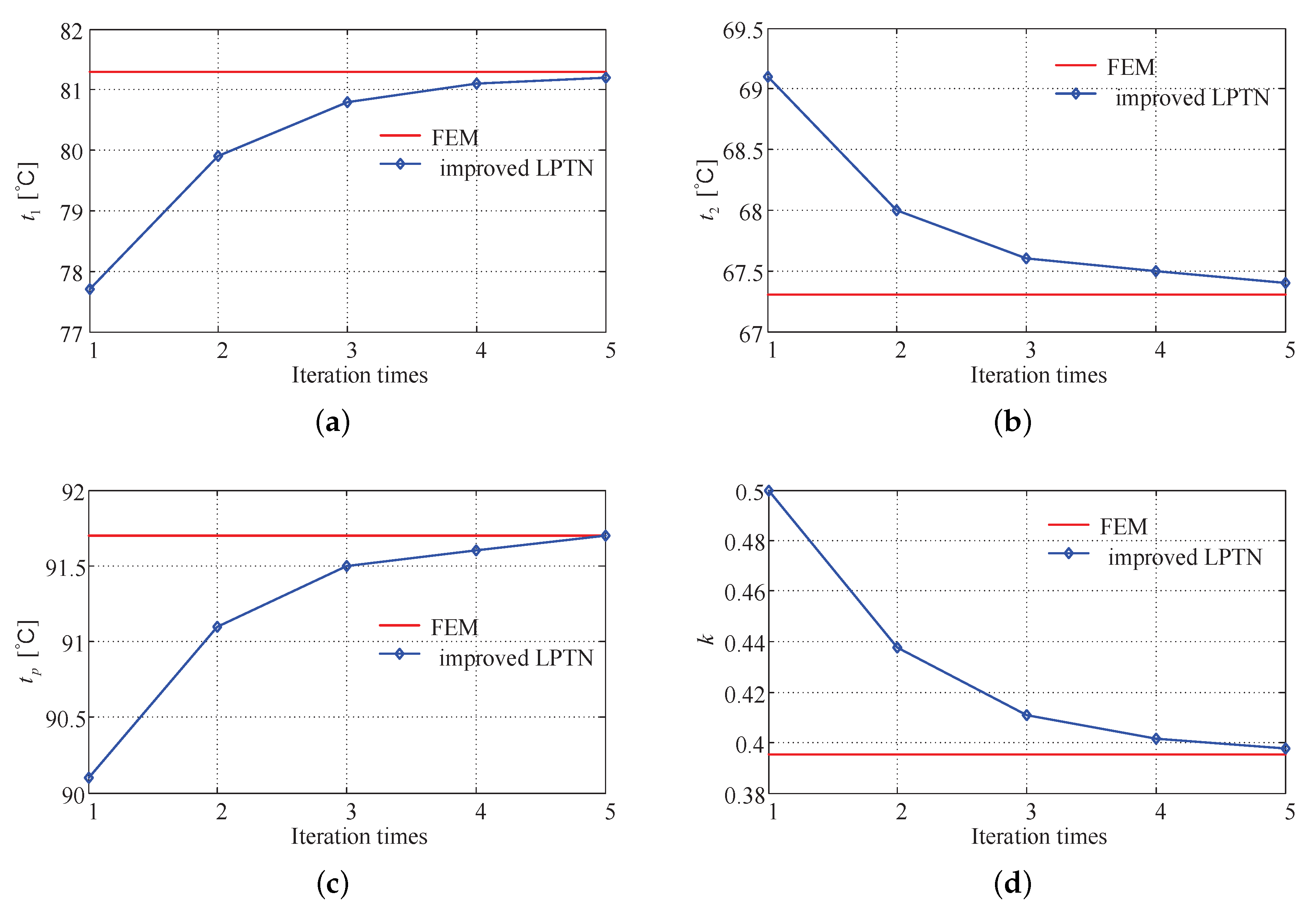
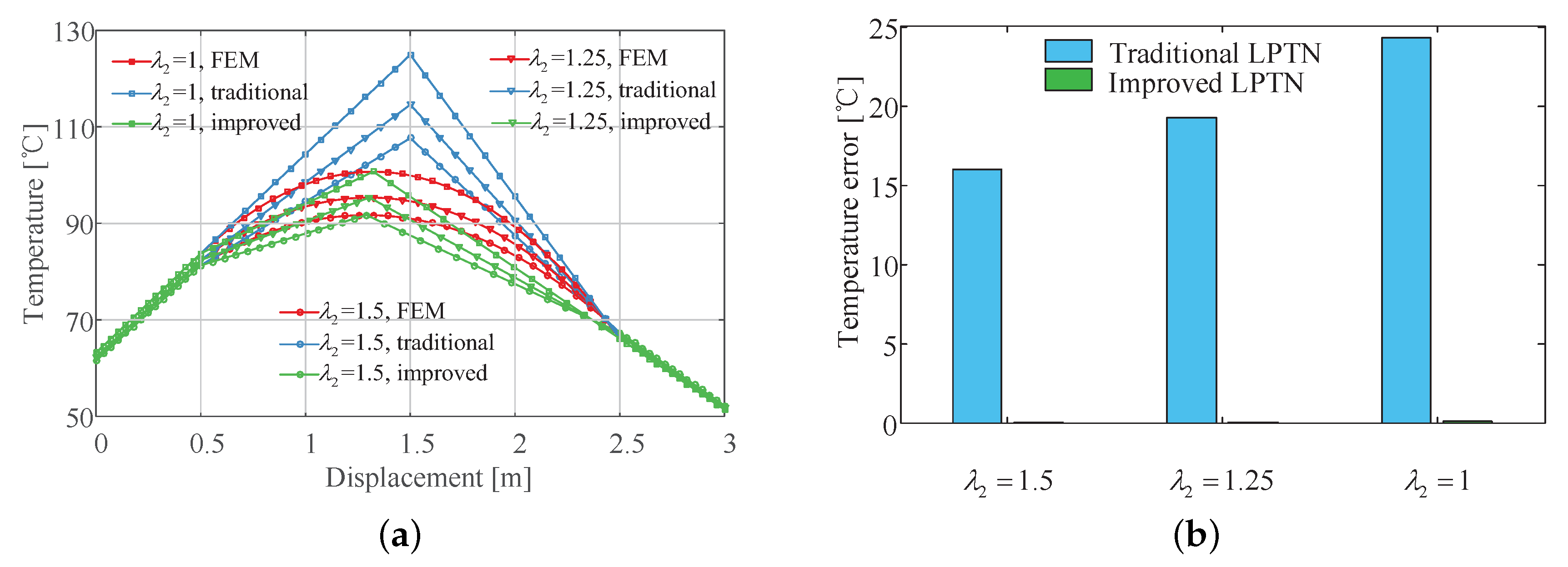
In this section, the accuracy of the improved LPTN is compared with that of traditional LPTN. The major parameters in simulation are listed in Table 1, and the results of the improved LPTN, the traditional LPTN and the numerical computation, are shown in Figure 6. They show that the traditional LPTN can describe the heat conduction well in the non-heat source regions (Regions I and III), but leads to over temperature in the heat source (Region II). The maximum temperature occurs at the midpoint of the heat source, which deviates from the FEM result. This large deviation is closely related to its misuse of the loading position and heat flux in the heat source. Conversely, the improved LPTN works well and achieves better results in both heat source and non-heat source regions. Thanks to the half-resistance theory, the over temperature disappears. In addition, benefit from Equation (12), loading position of the heat generator can be adjusted according to the nodes’ temperature. With iteration, accuracy of the location and temperature is further improved. As shown in Figure 7, details of the change of temperature and correction factor are recorded, in which and are boundary temperatures, is the maximum temperature and k is the correction factor. By the fifth iteration, both the maximum temperature and its location have reached a very high precision, with an error less than 1%. The improved LPTN successfully solves the two problems in the traditional LPTN; i.e., over temperature and incorrect location. It has significant advantage over the traditional LPTN in modeling the asymmetric heat dissipation, especially for those with low thermal conductivity heat sources. As shown in Figure 8, the lower thermal conductivity, the greater error of the traditional LPTN, while the improved LPTN can always predict accurately.
4. Implementation into U-Core Motor
4.1. Thermal Network Model
In this section, the improved LPTN method is implemented on a U-core motor to predict the temperature distribution. As shown in Figure 9, geometry of the U-core motor is presented. Each block is a cube, so the Cartesian coordinates are selected for the thermal path determination in both planes. According to the specific structure, only main thermal paths are retained in each plane. They are connected at intersecting nodes, and then expand the two-dimensional network to a spatial one. The basic 3-D element of that is shown in Figure 10.
Then, follow the thermal path shown in Figure 10 and connect these nodes; the improved LPTN for the U-core motor is established in Figure 11. It is a spatial network with 123 nodes in total. For easy identification, each thermal resistance is colored by the same color as the motor component, and different color lines are used to distinguish heat conduction in different directions. Besides, other auxiliary symbols, such as heat generator, ambient temperature and zero reference, are also illustrated in this figure.
Since all materials and dimensions of each block are known, the value of each thermal resistance is easily determined. The contact and convective thermal resistances can also be determined by empirical formulas [25] and identification method [26]. Their specific values are included in Appendix A. Besides, because the eight “current sources” all originate from the same winding, they share the same heat power density. So they can be determined according to their volume sizes. At 15 A, heating powers of each source are listed in Table 2.
4.2. Simulation and Analysis
A comparative study is conducted among the improved LPTN, traditional LPTN and FEM to verify the advantage of the improved LPTN. As shown in Figure 12, two splines are selected along the x and z directions on the motor, and then their temperatures are compared.
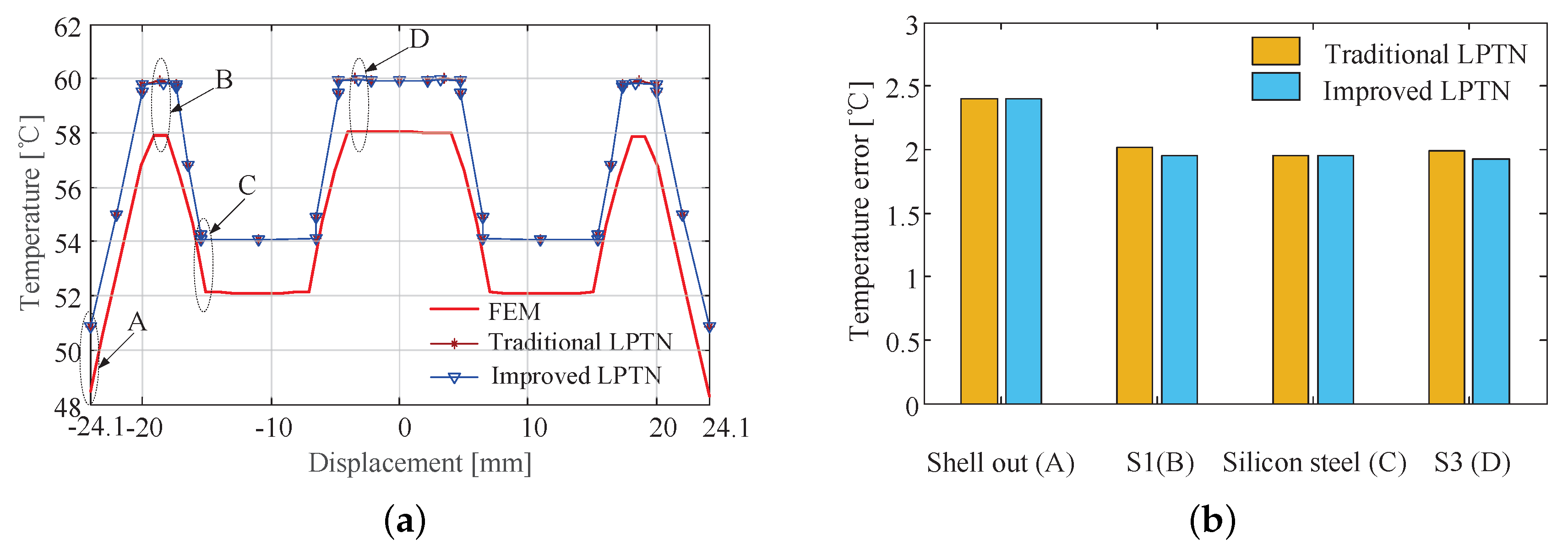
Figure 13 shows the results in x direction. Temperatures of the two LPTNs are almost the same; they both have a temperature error of 3 °C compared with the numerical result. Only at S1 and S2, locations of the heat generator, does the improved LPTN perform better, but the improvement is not obvious. There are two reasons for this result: one is the high thermal conductivity of winding; the other is the small thickness of winding in x direction. Both of them lead to a small thermal-resistance inside the heat source, and then advantages of the improved LPTN are weakened. However, the result still fits with the half-resistance theory and validates its effectiveness inside the heat source.
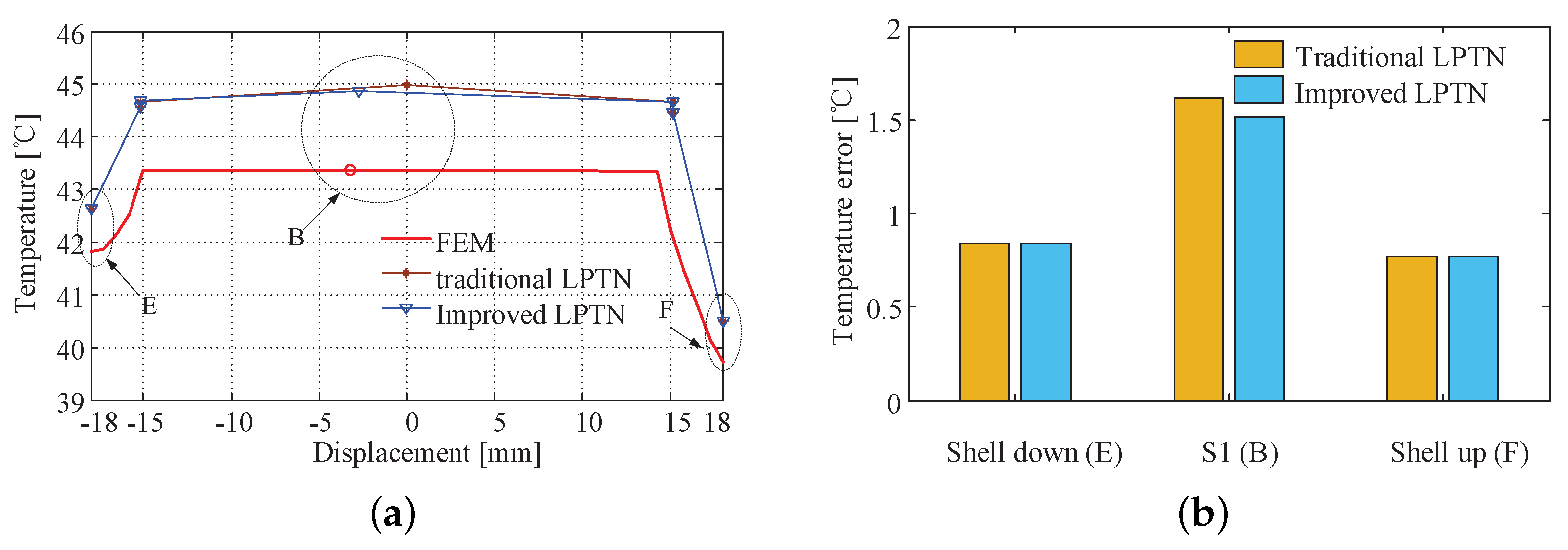
Figure 14 shows the comparison results in z direction. Because the uniform heat source is thicker in z direction, the improved LPTN performs better in z direction than x. It achieves a smaller temperature error at the heat generator, about 0.3 °C. Although the improvement in temperature prediction is not great, the improved LPTN has an absolute advantage in determining the loading position of heat generator. As shown in Figure 14c, with the increase of the number of iterations, location of the heat generator gradually approaches the real position. The introduction of the relationship between loading position and nodes’ temperature plays an important role for that.
In z direction, two more sets of comparisons are made at 10 A and 20 A. The results are shown in Figure 15 and Figure 16; they are consistent with the conclusion in Figure 14, which further confirms the advantage of the improved LPTN and illustrates that the simulation models are stable and reliable.
5. Experimental Validation
In this section, one prototype of U-core electric motor is presented, and experiments are conducted to validate the proposed improved LPTN.
5.1. Experimental Platform
A research prototype of pump motor is selected for experimental study. As shown in Figure 17a, it consists of a silicon steel sheet, permanent magnets, a winding, molded plastic, a rotating shaft, a shell, etc. Among these components, the winding is the main source of heat, wrapped in polystyrene resin on both sides of the U-shaped core. This embedded component has a negative effect on the heat dissipation and measurement, resulting in only the surface temperature can be measured directly by experiment. Therefore, the improved LPTN can only be validated by the experiment indirectly; i.e., utilize the experimental surface data to verify the FEM model first, and then validate the improved LPTN by the credible FEM model in heat source.
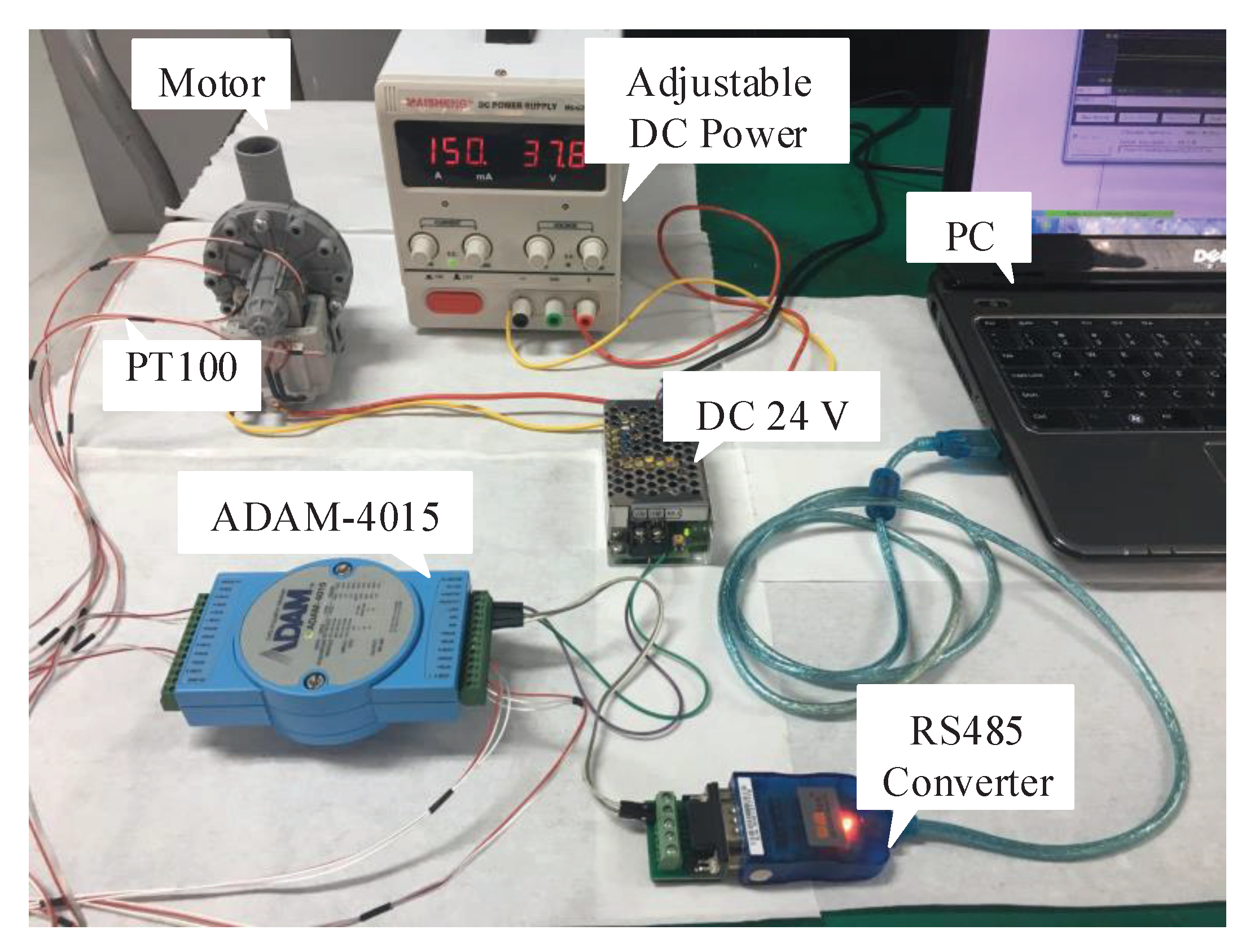
One test platform is structured for experimental validation, as shown in Figure 18. It includes a heat source, prototype, sensors and acquisition module. The adjustable DC power serves as the input of the uniform heat source, it can supply constant current to simulate the heating status under the condition of motor stall. Thermal sensors PT100 are shown in Figure 17b; they are attached on the motor to measure the temperature, and then collected by the ADAM-4015 module and transmitted to PC via the RS485 interface.
5.2. Experimental Results and Discussion
Consistent with settings in simulation, three groups of currents of 10, 15 and 20 A were used to validate the FEM model. After the temperature stabilized, temperatures of each point were recorded and presented in Figure 19. It can be seen that in three groups of test, the FEM model fits well with the results of the experimental measurement, and their errors are kept within 2 °C, indicating that the FEM model is exactly reliable and credible. Therefore, it is reasonable and scientific to validate the improved LPTN by the FEM model within the heat source. The conclusion in Section 4 has been validated indirectly, showing that the improved LPTN performs better than the traditional LPTN, especially in the uniform heat source with large thickness and low thermal conductivity.
6. Conclusions
In this paper, considering the change of heat flux in a uniform heat source, a novel improved LPTN is proposed to predict the thermal distribution more accurately. Compared with the traditional LPTN, the key achievements of this contribution are: 1. It reduces temperature error inside the heat source. Thanks to the compensation of the half-resistance theory, the lager heat flux is offset by the halved thermal resistance, ensuring the equilibrium of the temperature drop in the heat source without any negative impacts outside the heat source. 2. It determines the loading position of the heat generator; i.e., the maximum temperature position. Benefiting from the coupling relationship between the nodes’ temperature and the location of heat generator, the correction factor is derived, which is quite significant in asymmetric heat dissipation. It provides the chance for adjusting the loading position of the heat generator and redistributing thermal resistances. The iterative algorithm further strengthens the above advantages. Simulation and experiment are conducted on a U-core electric motor, and the results show that the improved LPTN fits with their results closely. Compared with the traditional LPTN, the improved LPTN can not only achieve higher accuracy for the maximum temperature prediction, but also determine its location.
Author Contributions
Conceptualization, B.L. and L.Y.; methodology, B.L. and L.Y.; software, B.L.; validation, B.L.; formal analysis, B.L.; investigation, B.L. and L.Y.; resources, B.L. and L.Y.; data curation, B.L.; writing—original draft preparation, B.L.; writing—review and editing, B.L., L.Y., W.C.; visualization, B.L.; supervision, L.Y.; project administration, L.Y.; funding acquisition, L.Y. All authors have read and agreed to the published version of the manuscript.
Funding
This research was funded by the National Key R&D Program of China under grant 2017YFB1300400, and the National Natural Science Foundation of China (NSFC) under grant 51875013 and 51575026.
Acknowledgments
The assistance from the Guangdong Walton Technology Co., Ltd. is gratefully acknowledged.
Conflicts of Interest
The authors declare no conflict of interest. The funders had no role in the design of the study; in the collection, analyses, or interpretation of data; in the writing of the manuscript, or in the decision to publish the results.
Abbreviations
The following abbreviations are used in this manuscript:
| LPTN | Lemped parameter thermal network |
| CFD | computational fluid dynamics |
| FEM | finite element method |
| TEFC | totally enclosed fan cooled |
| Temperature difference (°C) | |
| Thickness of the wall (m) | |
| Heating power () | |
| Thermal conductivity of medium I (W/m·K) | |
| Thermal conductivity of medium II (W/m·K) | |
| Thermal conductivity of medium III (W/m·K) | |
| Equivalent heat flux (s) | |
| Equivalent thermal resistance () | |
| A | Cross section area of heat flow () |
| Constant coefficient (-) | |
| Constant coefficient (-) | |
| Convective heat transfer on the left side of medium I (K) | |
| Convective heat transfer on the right side of medium III (K) | |
| k | Correction factor (-) |
| Boundary position between media I and II (m) | |
| Boundary position between media II and III (m) | |
| Boundary position of medium III (m) | |
| Q | Heat flow (J·s) |
| q | Heat flux (s) |
| Thermal resistance () | |
| t | Temperature (°C) |
| Ambient temperature (°C) |
Appendix A
Parameters in the thermal network are listed in Table A1.

Table A1.
Parameter Values in the Thermal Network.
| Name | Value | Name | Value | Name | Value | Name | Value |
|---|---|---|---|---|---|---|---|
| 52.9629 | 0.0016 | 0.0036 | 1.4233 × 10 | ||||
| 5.6167 × 10 | 1.5556 × 10 | 0.0036 | 5.7212 | ||||
| 408.4491 | 16.6860 | 16.2393 | 0.0841 | ||||
| 0.4861 | 298.6437 | 0.6481 | 8.5556 × 10 | ||||
| 885.7161 | 1.2307 | 0.6481 | 3.5000 × 10 | ||||
| 4.2940 | 1.4768 | 16.2393 | 2.7654 × 10 | ||||
| 4.2940 | 4.6765 | 0.0036 | 0.8711 | ||||
| 386.4556 | 4.6765 | 0.0036 | 0.8711 | ||||
| 0.5833 | 1.4768 | 35.0000 | 0.1628 | ||||
| 6.0602 × 10 | 1.2307 | 0.8711 | 0.7432 | ||||
| 881.3901 | 289.6437 | 0.0841 | 0.1628 | ||||
| 0.9348 | 0.9348 | 0.8711 | 0.7432 | ||||
| 298.6437 | 6.0602 × 10 | 3.5 × 10 | 35.0000 | ||||
| 1.2307 | 0.5833 | 8.5556 × 10 | 0.0036 | ||||
| 1.4768 | 881.3901 | 2.7654 × 10 | 0.0036 | ||||
| 4.6765 | 885.7161 | 0.1628 | 16.2393 | ||||
| 4.6765 | 4.2940 | 0.7432 | 0.6481 | ||||
| 1.4768 | 4.2940 | 0.1628 | 0.6481 | ||||
| 1.2307 | 386.4556 | 0.7432 | 16.2393 | ||||
| 298.6437 | 0.4861 | 5.7212 | 0.0036 | ||||
| 0.9348 | 5.6167 × 10 | 1.4223 × 10 | 0.0036 | ||||
| 0.5833 | 52.9629 | 86.7995 | 35.0000 | ||||
| 5.2790 | 408.4491 | 0.1427 | 0.0841 | ||||
| 0.4861 | 7.5223 | 0.2843 | 15.9856 | ||||
| 5.2790 | 282.7724 | 60.9119 | 750.1786 | ||||
| 1.3751 × 10 | 282.7724 | 1.4204 × 10 | 15.9856 | ||||
| 2.3932 | 7.5523 | 0.3737 | 750.1786 | ||||
| 215.3846 | 1.4204 × 10 | 0.0803 | 1.4211 × 10 | ||||
| 0.4861 | 82.9889 | 0.0803 | 82.9889 | ||||
| 5.2790 | 0.1405 | 41.7196 | 0.1405 | ||||
| 5.2790 | 0.1545 | 436.2265 | 0.1545 | ||||
| 5.2790 | 82.9889 | 436.2265 | 82.9889 | ||||
| 0.5833 | 1.4211 × 10 | 49.0389 | 1.4226 × 10 | ||||
| 0.9848 | 15.9856 | 0.3737 | 7.5523 | ||||
| 1.5556 × 10 | 750.1786 | 1.4204 × 10 | 282.7724 | ||||
| 1.5556 × 10 | 750.1786 | 86.7995 | 7.5523 | ||||
| 16.6860 | 15.9856 | 0.1427 | 282.7724 | ||||
| 1.5556 × 10 | 0.0841 | 0.1523 | 0.4884 | ||||
| 0.0016 | 35.0000 | 60.9119 | 22.0000 |
References
- Boglietti, A.; Cavagnino, A.; Staton, D.; Shanel, M.; Mueller, M.; Mejuto, C. Evolution and modern approaches for thermal analysis of electrical machines. IEEE Trans. Ind. Electron. 2009, 56, 871–882. [Google Scholar] [CrossRef] [Green Version]
- Staton, D.; Boglietti, A.; Cavagnino, A. Solving the more difficult aspects of electric motor thermal analysis in small and medium size industrial induction motors. IEEE Trans. Energy Convers. 2005, 20, 620–628. [Google Scholar] [CrossRef] [Green Version]
- Kefalas, T.D.; Kladas, A.G. Thermal investigation of permanent-magnet synchronous motor for aerospace applications. IEEE Trans. Ind. Electron. 2014, 61, 4404–4411. [Google Scholar] [CrossRef]
- Nategh, S.; Zhang, H.; Wallmark, O.; Boglietti, A.; Nassen, T.; Bazant, M. Transient thermal modeling and analysis of railway traction motors. IEEE Trans. Ind. Electron. 2019, 66, 79–89. [Google Scholar] [CrossRef]
- Arbab, N.; Wang, W.; Lin, C.; Hearron, J.; Fahimi, B. Thermal modeling and analysis of a double-stator switched reluctance motor. IEEE Trans. Energy Convers. 2015, 30, 1209–1217. [Google Scholar] [CrossRef]
- Abebe, R.; Vakil, G.; Calzo, G.L.; Cox, T.; Gerada, C.; Johnson, M. FEA based thermal analysis of various topologies for integrated Motor Drives (IMD). In Proceedings of the IECON 2015—41st Annual Conference of the IEEE Industrial Electronics Society, Yokohama, Japan, 9–12 November 2015. [Google Scholar]
- Craiu, O.; Machedon, A.; Tudorache, T.; Morega, M.; Modreanu, M. 3D finite element thermal analysis of a small power PM DC motor. In Proceedings of the 12th International Conference on Optimization of Electrical and Electronic Equipment, Basov, Romania, 20–22 May 2010; pp. 389–394. [Google Scholar]
- Trigeol, J.F.; Bertin, Y.; Lagonotte, P. Thermal modeling of an induction machine through the association of two numerical approaches. IEEE Trans. Energy Convers. 2006, 21, 314–323. [Google Scholar] [CrossRef]
- Wang, S.W.; Zhang, Y.; Hu, J.M. Thermal analysis of water-cooled permanent magnet synchronous motor for electric vehicles. Appl. Mech. Mater. 2014, 610, 129–135. [Google Scholar] [CrossRef]
- Dong, J.; Huang, Y.; Jin, L.; Lin, H.; Yang, H. Thermal optimization of a high-speed permanent magnet motor. IEEE Trans. Magn. 2014, 50, 749–752. [Google Scholar] [CrossRef]
- Zhang, Y.; Mcloone, S.; Cao, W.; Qiu, F.; Gerada, C. Power loss and thermal analysis of a mw high speed permanent magnet synchronous machine. IEEE Trans. Energy Convers. 2017, 32, 1468–1478. [Google Scholar] [CrossRef] [Green Version]
- Ulbrich, S.; Kopte, J.; Proske, J. Cooling fin optimization on a TEFC electrical machine housing using a 2D conjugate heat transfer model. IEEE Trans. Ind. Electron. 2018, 65, 1711–1718. [Google Scholar] [CrossRef]
- Mellor, P.H.; Roberts, D.; Turner, D.R. Lumped parameter thermal model for electrical machines of TEFC design. IEE Proc. B Electr. Power Appl. 1991, 138, 205–218. [Google Scholar] [CrossRef]
- Yabiku, R.; Fialho, R.; Teran, L.; Ramos, M.E.; Kawasaki, N. Use of thermal network on determining the temperature distribution inside electric motors in steady-state and dynamic conditions. IEEE Trans. Ind. Appl. 2010, 46, 1787–1795. [Google Scholar] [CrossRef]
- Dimolikas, K.; Kefalas, T.D.; Karaisas, P.; Papazacharopoulos, Z.K.; Kladas, A.G. Lumped-parameter network thermal analysis of permanent magnet synchronous motor. Mater. Sci. Forum 2014, 792, 233–238. [Google Scholar] [CrossRef]
- Rostami, N.; Feyzi, M.R.; Pyrhonen, J.; Parviainen, A.; Niemela, M. Lumped-parameter thermal model for axial flux permanent magnet machines. IEEE Trans. Magn. 2013, 49, 1178–1184. [Google Scholar] [CrossRef]
- El-Refaie, A.M.; Harris, N.C.; Jahns, T.M.; Rahman, K.M. Thermal analysis of multibarrier interior PM synchronous machine using lumped parameter model. IEEE Trans. Energy Convers. 2004, 19, 303–309. [Google Scholar] [CrossRef]
- Boglietti, A.; Carpaneto, E.; Cossale, M.; Vaschetto, S. Stator-winding thermal models for short-time thermal transients: Definition and validation. IEEE Trans. Ind. Electron. 2016, 63, 2713–2721. [Google Scholar] [CrossRef]
- Mohamed, A.H.; Hemeida, A.; Rasekh, A.; Vansompel, H.; Arkkio, A.; Sergeant, P. A 3D dynamic lumped-parameter thermal network of air-cooled YASA axial flux permanent magnet synchronous machine. Energies 2018, 11, 774. [Google Scholar] [CrossRef] [Green Version]
- Gerling, D.; Dajaku, G. Novel lumped-parameter thermal model for electrical systems. In Proceedings of the 2005 European Conference on Power Electronics and Applications, Dresden, Germany, 11–14 September 2005; pp. 1–10. [Google Scholar]
- Kuehbacher, D.; Kelleter, A.; Gerling, D. An improved approach for transient thermal modeling using lumped parameter networks. In Proceedings of the 2013 International Electric Machines & Drives Conference, Chicago, IL, USA, 12–15 May 2013; pp. 824–831. [Google Scholar]
- Gerling, D.; Dajaku, G. Thermal calculation of systems with distributed heat generation. In Proceedings of the 10th Intersociety Conference on Phenomena in Electronics Systems, San Diego, CA, USA, 30 May–2 June 2006; pp. 645–652. [Google Scholar]
- Li, K.; Wang, S.; Sullivan, J.P. A novel thermal network for the maximum temperature-rise of hollow cylinder. Appl. Therm. Eng. 2012, 52, 198–208. [Google Scholar] [CrossRef]
- Holman, J.P. Heat Transfer; Higher Education: New York, NY, USA, 2013; p. 5. [Google Scholar]
- Staton, D.A.; Cavagnino, A. Convection heat transfer and flow calculations suitable for electric machines thermal models. IEEE Trans. Ind. Electron. 2008, 55, 3509–3516. [Google Scholar] [CrossRef] [Green Version]
- Phuc, P.N.; Vansompel, H.; Bozalakov, D.; Stockman, K.; Crevecoeur, G. Inverse thermal identification of a thermally instrumented induction machine using a lumped-parameter thermal model. Energies 2019, 13, 37. [Google Scholar] [CrossRef] [Green Version]
Figure 1.
Typical case of heat conduction and diffusion.

Figure 2.
Equivalence of heat conduction and electric circuit.

Figure 3.
Heat flux for FEM, half power and traditional LPTN.

Figure 4.
Heat conduction within the heat source.

Figure 5.
The flow chart of the iterative model.

Figure 6.
(a) Temperature distribution in asymmetric heat dissipation with heat source. (b) Enlarged view of local area.
Figure 6.
(a) Temperature distribution in asymmetric heat dissipation with heat source. (b) Enlarged view of local area.

Figure 7.
(a) Curve of temperature with iterations. (b) Curve of temperature with iterations. (c) Curve of temperature with iterations. (d) Curve of correction factor k with iterations.
Figure 7.
(a) Curve of temperature with iterations. (b) Curve of temperature with iterations. (c) Curve of temperature with iterations. (d) Curve of correction factor k with iterations.

Figure 8.
(a) Temperature comparison with different thermal conductivities. (b) Temperature errors at maximum temperature.
Figure 8.
(a) Temperature comparison with different thermal conductivities. (b) Temperature errors at maximum temperature.

Figure 9.
(a) Cross section of the electric motor in XY plane. (b) Cross section of the electric motor in XZ plane.
Figure 9.
(a) Cross section of the electric motor in XY plane. (b) Cross section of the electric motor in XZ plane.

Figure 10.
Basic 3-D elements of the thermal network of the heat source.

Figure 11.
Thermal network of the whole motor.

Figure 12.
(a) Test spline in x direction. (b) Test spline in z direction.

Figure 13.
(a) Temperature distribution in x direction at 15 A. (b) Temperature error at several points.
Figure 13.
(a) Temperature distribution in x direction at 15 A. (b) Temperature error at several points.

Figure 14.
(a) Temperature distribution in z direction at 15 A. (b) Temperature error at several points. (c) Curve of correction factor k with iterations.
Figure 14.
(a) Temperature distribution in z direction at 15 A. (b) Temperature error at several points. (c) Curve of correction factor k with iterations.

Figure 15.
(a) Temperature distribution in z direction at 10 A. (b) Temperature error at several points.
Figure 15.
(a) Temperature distribution in z direction at 10 A. (b) Temperature error at several points.

Figure 16.
(a) Temperature distribution in z direction at 20 A. (b) Temperature error at several points.
Figure 16.
(a) Temperature distribution in z direction at 20 A. (b) Temperature error at several points.

Figure 17.
(a) Structure of the U-core motor. (b) Distribution of measurement points.

Figure 18.
Experimental platform for temperature test.

Figure 19.
(a) Temperature at test points. (b) Temperature error at test points.

Table 1.
Major parameters for the simulation.
| Symbol | Quantity | Vaule | Unit |
|---|---|---|---|
| Length | 0.5 | m | |
| Length | 2.5 | m | |
| Length | 3 | m | |
| Thermal conductivity of medium I | 1 | W/m·K | |
| Thermal conductivity of medium II | 1.5 | W/m·K | |
| Thermal conductivity of medium III | 2 | W/m·K | |
| Convective heat transfer on left | 1 | W/mK | |
| Convective heat transfer on right | 2 | W/mK | |
| Heating power | 50 | W/m | |
| Ambient temperature | 22 | °C |
Table 2.
Heat source power for simulation.
| Name | Value | Unit | Name | Value | Unit | Name | Value | Unit |
|---|---|---|---|---|---|---|---|---|
| S1 | 0.8992 | W | S4 | 0.5183 | W | S7 | 0.8992 | W |
| S2 | 0.5183 | W | S5 | 0.8992 | W | S8 | 0.5183 | W |
| S3 | 0.8992 | W | S6 | 0.5183 | W | Total | 5.67 | W |
© 2020 by the authors. Licensee MDPI, Basel, Switzerland. This article is an open access article distributed under the terms and conditions of the Creative Commons Attribution (CC BY) license (http://creativecommons.org/licenses/by/4.0/).
Share and Cite
MDPI and ACS Style
Li, B.; Yan, L.; Cao, W. An Improved LPTN Method for Determining the Maximum Winding Temperature of a U-Core Motor. Energies 2020, 13, 1566. https://0-doi-org.brum.beds.ac.uk/10.3390/en13071566
AMA Style
Li B, Yan L, Cao W. An Improved LPTN Method for Determining the Maximum Winding Temperature of a U-Core Motor. Energies. 2020; 13(7):1566. https://0-doi-org.brum.beds.ac.uk/10.3390/en13071566
Chicago/Turabian StyleLi, Bin, Liang Yan, and Wenping Cao. 2020. "An Improved LPTN Method for Determining the Maximum Winding Temperature of a U-Core Motor" Energies 13, no. 7: 1566. https://0-doi-org.brum.beds.ac.uk/10.3390/en13071566
Note that from the first issue of 2016, this journal uses article numbers instead of page numbers. See further details here.