1. Introduction
In recent years, green energy has gradually gained attention due to raising awareness of environmental protection. Many clean and pollution-free energy sources (such as wind power, solar power, and hydropower) have been attracting attention and are widely used for electricity production in many countries. In particular, wind power is developing rapidly, and many large wind farms have been built to harvest the energy from the wind in offshore and onshore areas.
In the past years, many previous studies involving single wind turbines have been completed through various research methods such as field measurements [
1,
2], wind tunnel experiments [
3,
4], and numerical simulations [
5,
6]. Some studies focused on investigating changes in the wake characteristics of wind turbines exposed to different incoming mean velocities [
7,
8] and different inflow turbulence intensity levels resulting from surface roughness change [
6,
9] and thermal stability [
10,
11]. Significant findings include that the incoming flow with intense turbulence levels, whether induced by surface roughness or thermal buoyancy, can effectively facilitate the wake recovery rate that is along with the generation of large turbulence intensity and strong momentum flux. Turbine rotors operating at the same tip speed ratio (TSR) λ but different incoming mean velocities [
8] produce wakes that have consistent features in terms of normalized wake deficits and turbulence enhancement. The blades of a turbine under different freestream inflow velocities [
7] induce the generation of a tip vortex system where the vortex completely breaks down immediately downstream of the rotor operating at a higher TSR (about 12) or collapses further downstream of the turbine with a certain distance up to 10 rotor diameters at a lower TSR (about 7) condition. The above two studies indicate that changing the TSR can lead to significant effects on the characteristics of turbine wakes.
In recent decades, wind tunnel experiments have been widely applied to study the structure and characteristics of small wind turbine wakes using velocimetry, including Cobra probes, Hot-wire probes, and Particle image velocimetry (PIV). Wind tunnel experiments carried out by Iungo [
12], Mallipudi et al. [
13], Chawla et al. [
14], Wang et al. [
15], and Wu et al. [
16] adopted Cobra probes to collect complex unsteady wakes originated from turbines, rotating objects, and airfoils. Iungo [
12] conducted wind tunnel tests with the Cobra probe, and found that the axial velocity component is characterized by a significant wake velocity deficit, which gradually recovers to the incoming wind velocity at further downstream locations, and the vortex generated from near the hub is wholly diffused at downstream distances of more than four rotor diameters. Chawla et al. [
14] conducted wake measurements of airfoils by employing the Cobra probe to understand the wake characteristics and then facilitate the improvement of the airfoil efficiency through a suction control. Mallipudi et al. [
13] used the Cobra probe to examine the wake characteristics of stationary and rotating objects. They conducted an in-situ calibration through the comparison of the manufacturer specifications and then confirmed that the Cobra probe could achieve accuracies of wind speed within 0.5 m s
−1, wind direction less than 1 degree in yaw and pitch, and a sufficient sampling frequency up to approximately 1500 Hz. Wang et al. [
15] used the Cobra probe and PIV to examine unsteady wakes from a single-rotor turbine and a twin-rotor turbine in the wind tunnel experiment. The comparison of the wake measurements in the near wake region at x/d = 2 showed good agreement (here, x and d denote the streamwise position and the rotor diameter, respectively). Wu et al. [
16] compared measurements of stand-alone turbine wakes collected from the Cobra probe and the Hot-wire probe and presented the wakes that have a reasonably consistent structure and characteristics in terms of mean wake velocity and turbulence intensity. Based on the above-mentioned previous studies, the Cobra probe has become a widely-used and reliable velocimeter appropriate for measurements of complex turbine wakes in a wind tunnel.
A real utility-scale wind turbine has a pitch regulation system to control the blade rotating speed. Generally, a turbine pitch regulation system keeps the blade rotating speed as a constant as inflow velocity is greater than 10 m s
−1 (e.g., Vestas V80). Hence, a turbine TSR decreases as the inflow wind speed increases, although the blade rotating speed does not change. Studies involving the estimation of the turbine power coefficient have also been extensively conducted in wind tunnel experiments [
4,
17,
18,
19] and field measurements [
20]. Their results consistently show that the power coefficient as a function of the TSR has a parabolic distribution with a maximum of about 0.3–0.45 between TSR = 4 and TSR = 8. Some studies present that the shaft torque as a function of the blade angular velocity has a similar parabolic distribution with the maximum at a blade angular velocity. These results indicate that the initial increase of the blade rotation speed can raise the blade generating shaft torque and the power generation efficiency, but too high blade rotation speeds lead to a reduction in the torque and power generation efficiency. This behavior illustrates open issues related to turbine pitch regulation strategy, in particular the optimal strategy to target the maximum power coefficient, the maximum shaft torque, or a higher blade angular velocity with a moderate shaft torque. A series of wake measurements under different TSR conditions is still lacking, and the relationship with the power generation efficiency is not well understood. A previous study by Dilip and Porte-Agel [
21] showed that pitch regulation, which is applied to adjust the blade angular velocity of the upstream turbines with a decreased pitch angle of −2 degrees (i.e., changes the original TSR of the rotor) in the in-line two-turbine simulations, can mitigate the wake effects on the downstream turbines and increases the total power output by 2.8% at a lower inflow turbulence condition. Such a strategy can be viewed as an alternative to increasing the power produced in a massive wind farm operation in the future.
Some of the studies mentioned above [
8,
9,
10,
11,
12] have conducted wind tunnel experiments focusing on the stand-alone wind turbine wake characteristics under the influence of surface roughness change, surface temperature variation, and different incoming wind velocities. However, these studies did not further systemically investigate the relationship between the power generation efficiency and the wake characteristics. A detailed investigation of the wake characteristics of the single turbine and its power generation efficiency at the different TSR conditions is still lacking. Therefore, this study conducted a wind tunnel experiment to examine power generation efficiency and wake characteristics of a stand-alone turbine operating at different blade angular velocities under the same incoming mean wind velocity.
Section 2 details the set-up of the wind tunnel experiment, the information on the miniature wind turbine model, and the specification of the selected measuring instruments.
Section 3 discusses the results and methods used to estimate the torques, the power output, and the power coefficient. Vital turbulence statistics, including the mean streamwise and vertical velocities, the turbulence intensity, and the momentum flux, as well as a comparison of results under the different blade angular velocities, are presented and discussed in
Section 4. A summary is given in
Section 5.
2. Experimental Setup
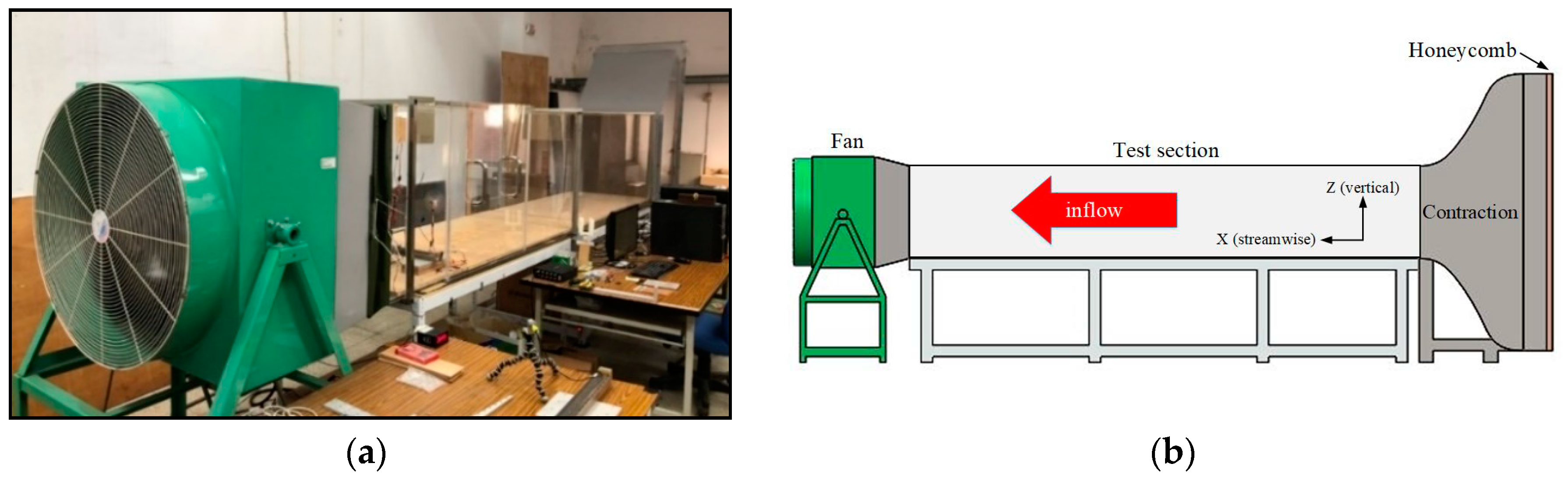
The experiment was conducted in an in-house open-type wind tunnel (shown in
Figure 1) located in the basement at the Department of Engineering Science, National Cheng Kung University, Tainan, Taiwan. The test section size of this tunnel is 4.4 m in length, 0.8 m in width, and 0.8 m in height. The wind-making facility includes an SFBM-36D fan made by the Shuenn Farn Ventilator Industrial Co. and a VFD-S frequency converter from Delta. The fan is placed downstream of the tunnel to suck the airflow passing through the test section. The VFD-S frequency converter is used to control the fan rotation speed with a prescribed frequency of 10–60 Hz, so that the incoming flow velocity inside the test section can be adjusted from 1 to 10 m s
−1.
In the experiments, the air temperature in the basement was controlled at 25 °C by two air conditioners. A constant frequency of 30 Hz was set in the VFD-S frequency converter to produce the freestream velocity of about 6.1 m s
−1 in the test section of the tunnel. We chose the Maxon DCX-12-L motor as the turbine dc generator driven by a 15-cm-diameter rotor made by a ProJet 3510 3D printer inside the tunnel.
Table 1 lists some Maxon DCX-12-L motor information. The blade airfoil is NACA 0012. The blade chord length and twist angle are optimized using the blade element momentum theory. The blade geometry information is given in
Table 2, and the detailed design procedure of the turbine rotor are given in the work of Wu et al. [
16].
In this study, the experimental goal was to systemically investigate the relationship between the turbine power generation efficiency and the wake characteristics at different TSR conditions under the same hub-level incoming velocity of 6.1 m s−1. Estimates of the power coefficient at different TSRs were needed for evaluating the turbine power generation efficiency, which required a further examination of the actual power output and the friction-induced power losses. To achieve this goal, the Maxon DCX-12-L motor was used as the turbine generator and connected to a resistor and a dc voltmeter in a series circuit. The resistor could be adjusted to achieve the turbine blade rotating at the different angular velocities (i.e., different TSRs) under the same hub-level incoming velocity. The TSRs considered are: 0.9, 1.5, 3.0, 4.1, 5.2, and 5.9. A dc voltmeter was used to measure the total resistance and the current in the circuit at each TSR condition. A Cobra probe was used to measure the three velocity components (streamwise, spanwise, and vertical) at positions across the turbine wakes and the inflow velocity.
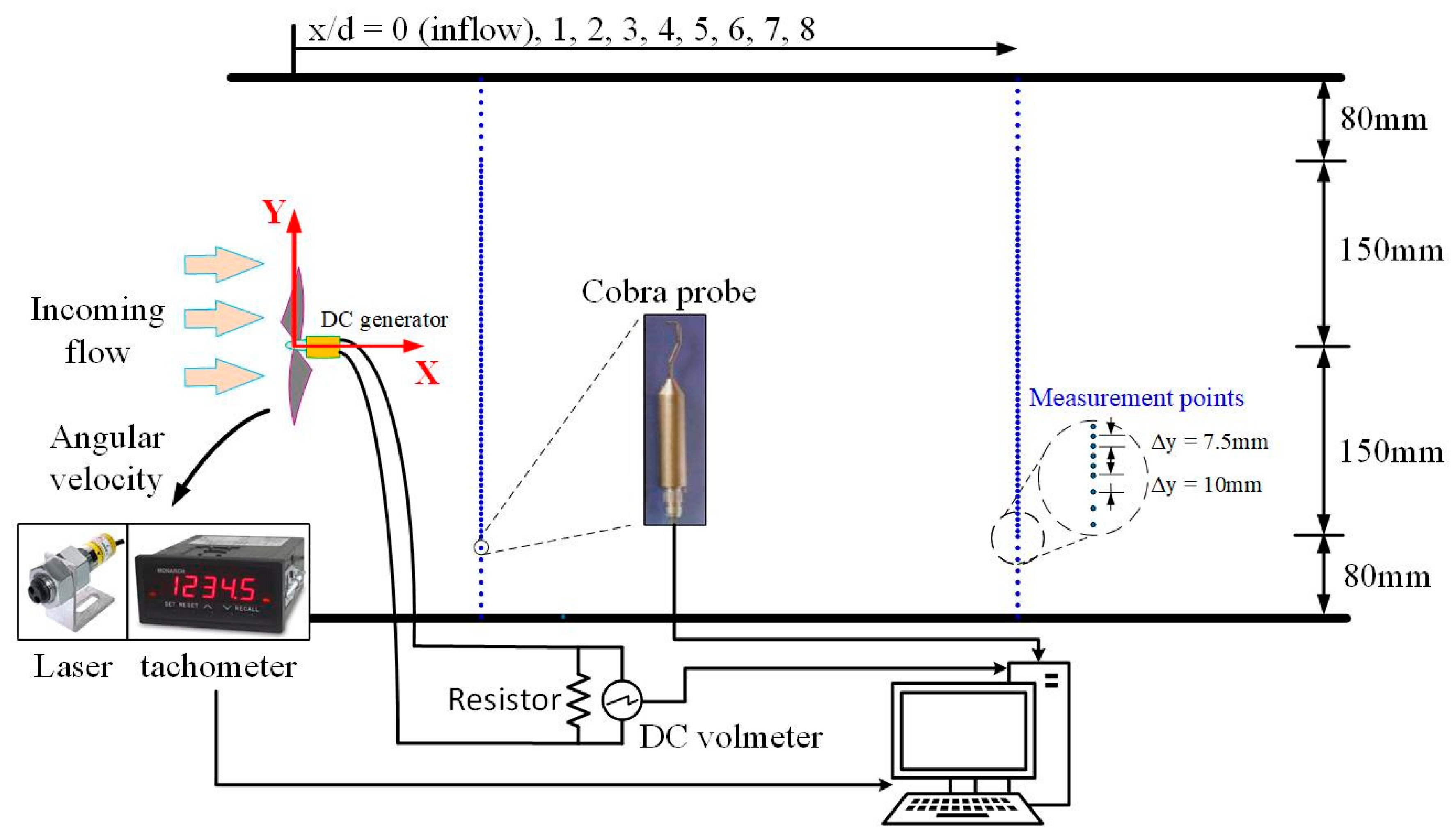
Figure 2 shows the measuring chain schematic. Measurements taken in the experiment include the instantaneous flow velocity components (streamwise, spanwise, and vertical), the blade angular velocity, the generator-produced electric current, and the total resistance of the circuit. The three velocity components were measured using a calibration-free, 4-hole Cobra probe manufactured by Turbulent Flow Instrument. The Cobra probe was positioned at the turbine hub level to collect the instantaneous wind speed data laterally from y = −230 to 230 mm (with intervals of 7.5 mm from y = −150 to 150 mm and intervals of 10 mm from y = −230 to −150 mm and from y = 150 to 230 mm) at the streamwise locations of x/d = 1, 2, 3, 4, 5, 6, 7, and 8 as well as at the inflow (at x/d = 0 without the model turbine placement), as shown in
Figure 2. The measurements for each TSR condition have a total of 513 measurement points, and the measuring time was 120 s, with a sampling rate of 1200 Hz on each point. The actual measuring period for each case was approximately 24 h. The blade angular velocity was measured using an ACT-3X series panel tachometer equipped with the ROLS24-W remote optical laser sensor from Monarch Instrument. The electric current and the total resistance in the circuit were measured by a digital dc Voltmeter.
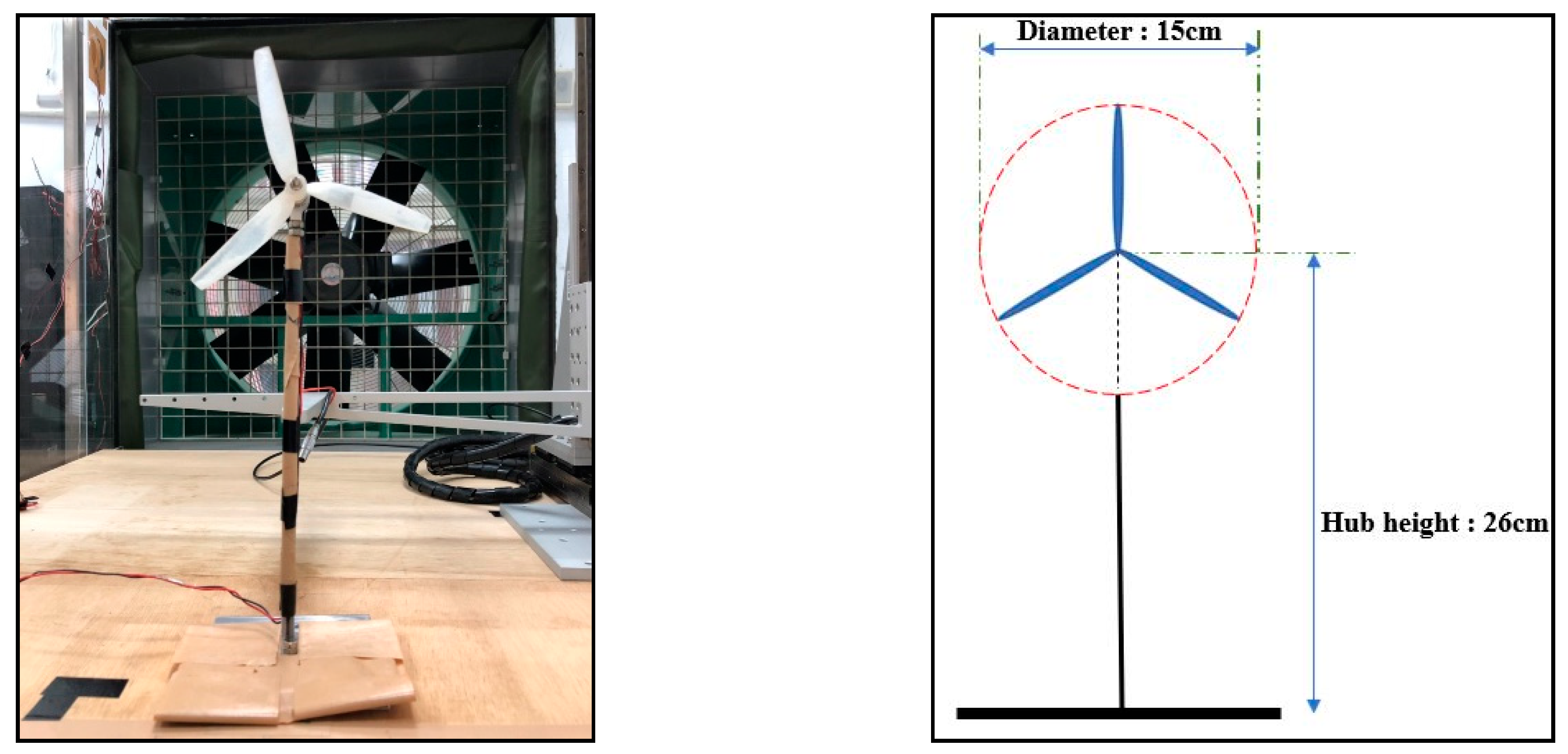
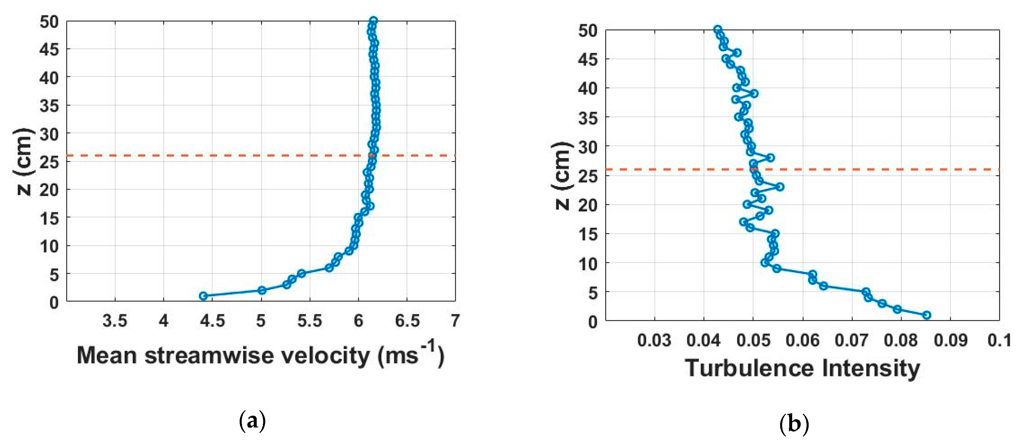
Figure 3 shows a picture of the small wind turbine placed in the wind tunnel. The turbine rotor has a diameter of 15 cm and a hub height of 26 cm. Vertical profiles of the inflow mean velocity and the turbulence intensity (measured at x/d = 0 and y/d = 0 without the model turbine placement) are presented in
Figure 4. Here, the mean streamwise velocity was set to approximately 6.1 m s
−1, and the turbulence intensity was around 5%. The turbulence intensity (TI) is defined as follows:
where
= 6.1 m s
−1 is the incoming mean velocity at the hub height and (
,
,
) denote the velocity variance components in the streamwise, spanwise, and vertical directions, respectively. In Equation (1), TI can be considered as the “total” turbulence intensity, which is composed of streamwise turbulence intensity I
u =
⁄
, spanwise turbulence intensity I
v =
⁄
, and vertical turbulence intensity I
w =
⁄
. The turbulence intensity is an index that can be used to quantify the magnitude of the turbulence properties.
During the experimental measurements, the generator was connected to a resistor and a dc Voltmeter in a series circuit, where the adjustment of the resistor could control the blade angular velocity by changing the load of the circuit (i.e., altering the total resistance of the circuit) under the same incoming speed. Here, we selected six different resistors to bring about total resistances R
t of 9.5, 10.5, 10.9, 14.4, 31.2, and 88.8 ohms (given in
Table 3) in the circuit, which led to the blade angular velocities Ω of approximately 675, 1134, 2358, 3199, 4060, and 4558 rpm, respectively. These blade angular velocities corresponded to the different TSRs of 0.9, 1.5, 3.0, 4.1, 5.2, and 5.9. In the experiments, the Reynolds number (based on the incoming mean velocity at the hub height
and the turbine rotor diameter
) was Re
d =
. The chord-based Reynolds number, Re
chord =
(based on the average chord
about 0.01 m and the blade tip speed
), varied from
at a TSR of 0.9 to
at a TSR of 5.9. Moreover, statistics of wake measurements and estimations of power coefficients with and without the consideration of the friction-induced losses are the main focus of this study and presented next.
3. Power Output Estimation
In the wind turbine operation, the mechanical power
is a sum of the power output
and the friction-induced power loss
. There are three methods to calculate the mechanical power
. One is obtained from the product of the shaft torque
and the blade angular velocity
based on the blade element momentum theory. Another is computed from the product of the torque constant
, the electrical current
, and the blade angular velocity
. The third is from the product of the inertia of the moment
, the blade angular acceleration
, and the blade angular velocity
[
22,
23,
24]:
It should be pointed out that in Equation (2) the friction-induced power loss exists in the mechanical torque as the airflow drives the blade rotation. This loss has resulted from the friction of the generator shaft
and the friction of the blade surface
, which leads to mechanical torque as follows:
where
is the electromagnetic torque. Application of
to
,
, and
leads to
where
is the electromagnetic torque constant,
where
is the friction-induced torque loss from the generator shaft,
where
is the friction-induced torque loss from the blade surface. The actual power output of a wind turbine can be estimated from the product of voltage
and current
in the circuit, which leads to the two following equations to compute the electromagnetic torque
and the electromagnetic torque constant
by
In Equations (7) and (8), the electrical current, the total resistance, and the blade angular velocity were measured in the experiment. A linear regression of
and
can obtain the equation
with a determination coefficient of 0.996. Note that the
unit is a millinewton meter (i.e.,
). Besides, the power coefficient (C
P) of a wind turbine is a common index to quantify the performance of power output at an operating condition and is defined as
where
is the density of the air, and
is the rotor-swept area. The estimated power coefficients of the turbine at the different TSRs are given in
Table 3.
Estimates of the two friction-induced torque losses (
and
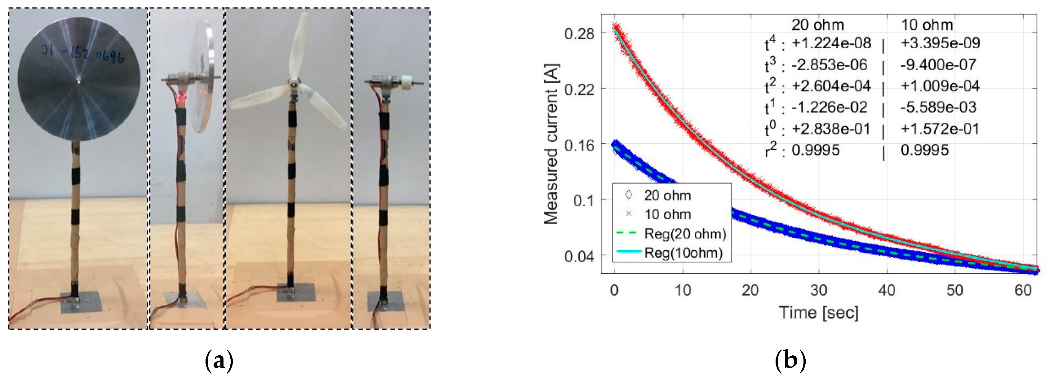
) require two separate testing experiments. The first testing experiment was to mount a circular aluminum disk on the generator shaft (see
Figure 5a). The selected disk has a weight
and a radius
. The inertia of momentum for a circular disk can be calculated by
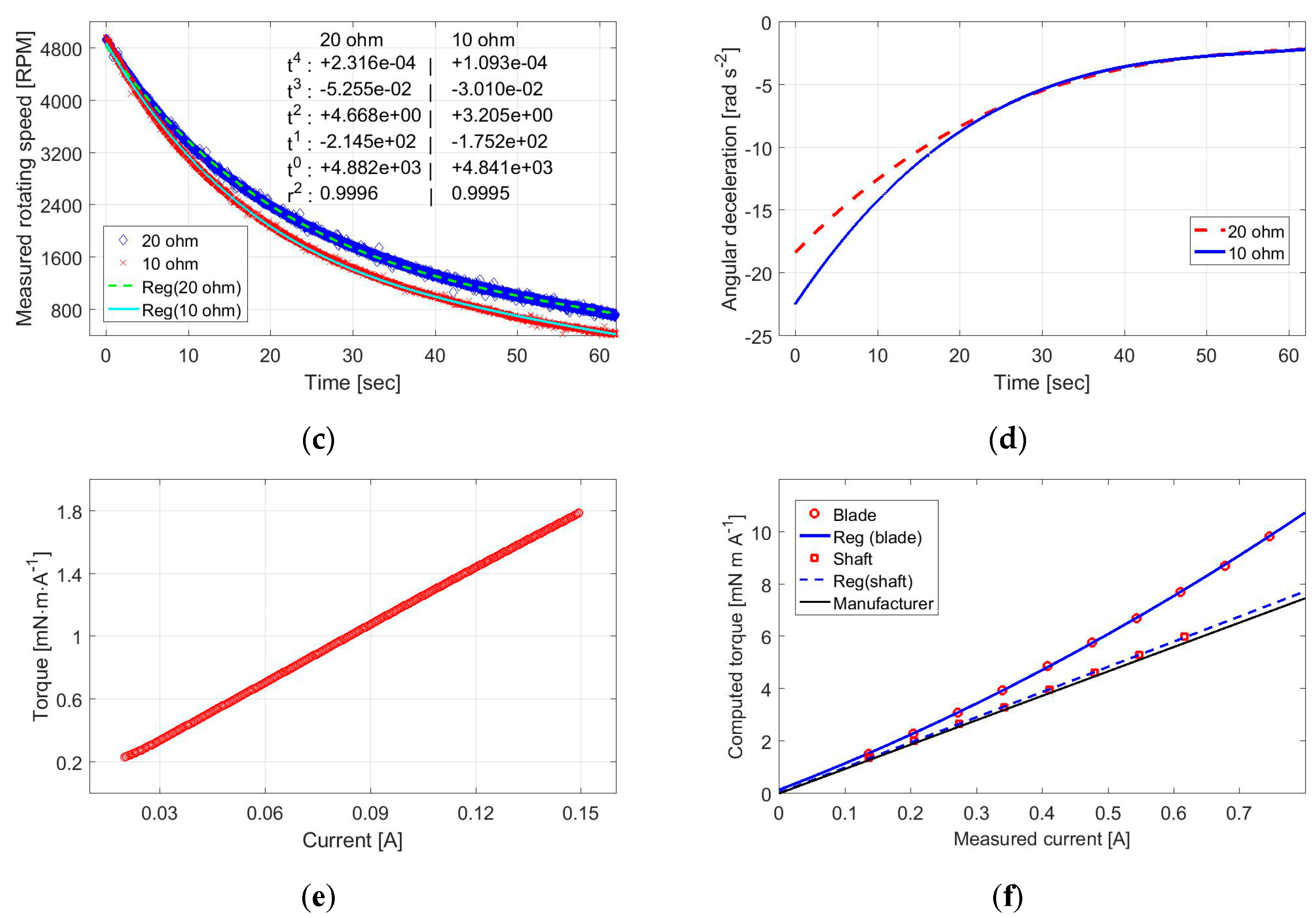
. During the experiment, we used a direct current power supply (DCPS) to provide the current to the motor to raise the rotating speed of the disk to above 5000 RPM, and then switched to the generator state to record time series data of the electrical current and the rotation speed. Two resistors with 10 and 20 ohms were individually loaded to the generator. The time series data of the electrical current and the rotation speed for the two resistors are shown in
Figure 5b,c. To get rid of spikes in the measured data, continuous electrical current and rotating speed distributions were constructed by a polynomial regression (the polynomial coefficients given in
Figure 5b,c) and then used in the torque constant estimation. The angular deceleration of the disk was estimated from the differential of the rotating speed regression polynomial and shown in
Figure 5d. In Equation (5),
can be considered as a function of the disk weight
and given in the following
where
is a frictional coefficient. In the generator state, the inertia of momentum from the aluminum disk drove the shaft rotation and induced the shaft friction, resulting in the following equation
To calculate
and
, a rotating speed
is selected to find the time
for 10 ohms and
for 20 ohms in
Figure 5c. In
Figure 5b,d, we can find
and
at
and
and
at
, and bring them into Equation (11), resulting in the following equations
Solving Equation (12) can obtain the following
The estimation of the torque constant is about 8.487
, which is similar to the computed torque constant value (i.e., 7.830) of the generator with the rotor. The torque-current regressed equation (as shown in Equation (4)) is
. It should be pointed out that this test was done using the aluminum disk with a weight
. For proper application to the model turbine, we have to adopt the rotor mass
(approximately 20 g) to compute the friction-induced torque loss from the generator shaft, resulting in
In
Figure 5e, the friction-induced torque loss around the shaft is regressed to
. Here, the
unit is a millinewton meter (i.e.,
).
In the second testing experiment, a DCPS was used to supply electricity to the motor to examine the torque constants of the motor mounting with the turbine rotor and the rotor shaft separately (shown in
Figure 5a). The rotating speed and both given current and voltage from the DCPS were measured to compute the mechanical torque that was later used for regression with the given current to calculate the torque constant (see
Figure 5f). As given in
Table 1, the manufacturer-provided torque constant is 9.66
at the shaft-no-load condition. For the rotor shaft condition, the regressed equation is
, which has a good agreement with the manufacturer-provided torque constant. For the turbine rotor condition, a second-order polynomial was used for a better fit to have the regressed equation
. The
could be estimated from the difference of
and
, leading to
. Finally, the
calculation could sum up
,
, and
to acquire the equation
, which was used to calculate the mechanical torque and the mechanical power coefficient (given in
Table 3).
In
Table 3, the TSR can be converted directly from the blade angular velocity (with a unit RPM) times a factor of 1.288 × 10
−3 (computed from 2π/60·R/
= 2π/60·0.075/6.1). Hence, the angular velocities of 1000, 2000, 3000, and 4000 RPM correspond to the TSRs of approximately 1.3, 2.6, 3.9, and 5.2, respectively.
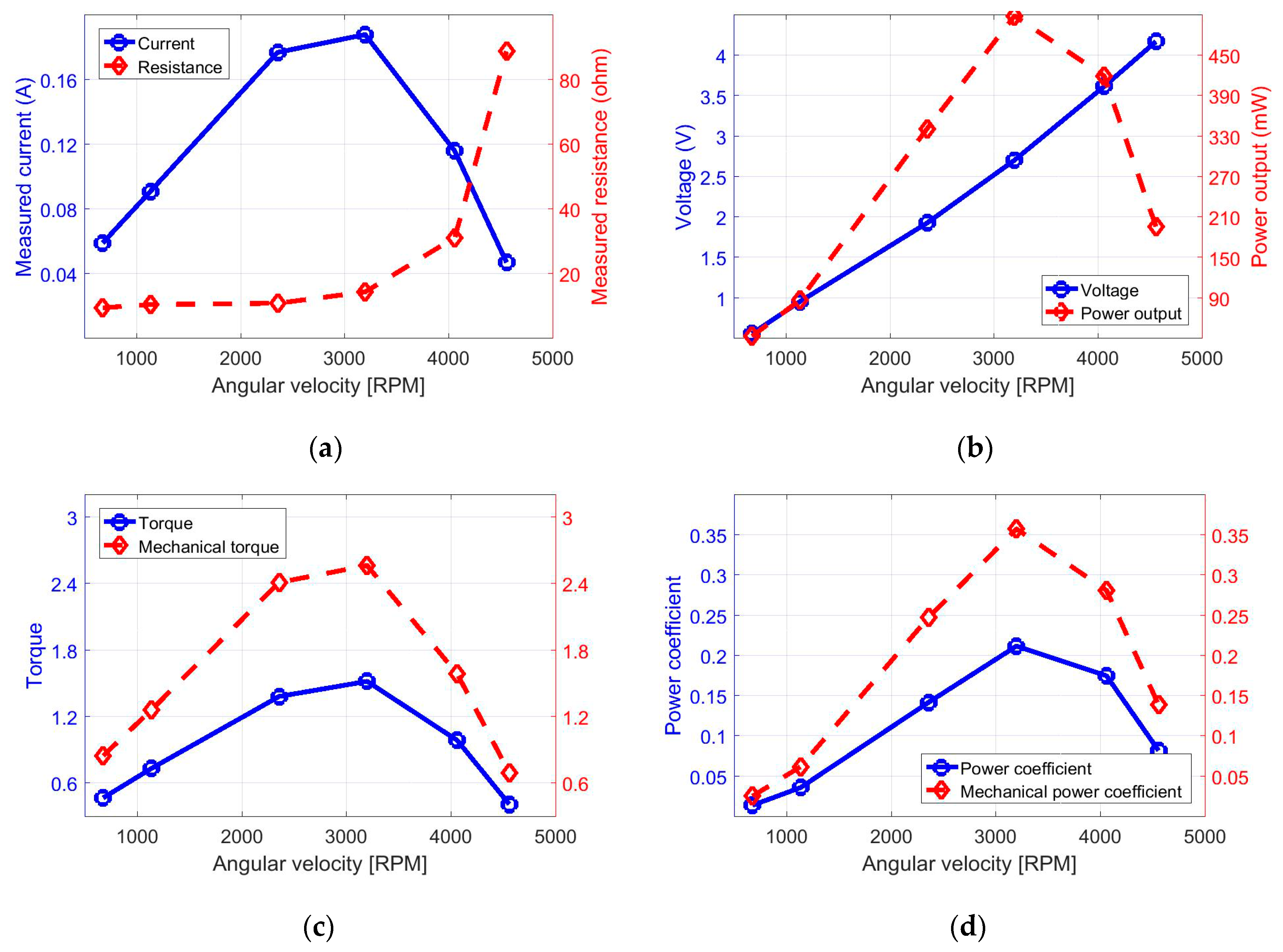
Figure 6 has four subplots containing the relationships of the measured electrical current, the measured total resistance, the estimated generator voltage, the computed power output, the calculated torque, the estimated torque constant, and the power coefficient with respect to the blade angular velocity. As shown in
Figure 6a, the measured current increases and then decreases with the increment of the blade angular velocity. The maximum current of 0.188 A occurs at the C4 condition (TSR = 4.1), whereas the relatively lower currents (less than 0.06 A) appear at both the low and high blade-rotating conditions (i.e., C1 and C6). Besides, the measured currents are found to increase with total resistance at the conditions of TSR ≤ 4.1 (with R
t ≤ 14.4 ohms). At the conditions of TSR = 5.2 and 5.9, the measured currents have an obvious decrease due to the overload with the total resistance of 31.2 and 88.8 ohms in the electrical circuit. This result indicates that the selected turbine generator is suitable for a load of approximately 15 ohms or less in the circuit to achieve the maximum allowable power output. The presence of the overload to the generator breaks down the quasi-steady approximation of electromagnetism to cause the emission of electromagnetic radiation, which leads to the magnet of the generator to lose energy.
Figure 6b shows the distributions of the computed voltage and power output of the generator. The voltage is obtained from the product of the measured current and total resistance and is found proportional to the blade angular velocity with a regression function of V(Ω) = (9.202 Ω − 1272) × 10
−4 and a coefficient of determination 0.996. The voltage trend demonstrates that the increased blade rotating speed can effectively increase the voltage difference by the generator, which is completely different from the distributions of the measured current and the power output. The power output (shown in
Figure 6b) is obtained from the product of the measured current and the voltage and has a maximum of 509 milli-Watt (mW) at the C4 condition with the TSR of 4.1. Moreover, the TSR increments between C3 and C4 as well as between C4 and C5 are almost the same. The data comparison between C3 and C5 shows that the C3 condition has a larger current generation in the circuit, whereas the C5 condition has a greater voltage difference from the generator (due to its higher blade angular velocity). The power output at C5 (TSR = 5.2) is relatively larger than that at the TSR of 3.0. This result indicates that the generator can produce more electrical power in the case of a higher blade rotating speed, with a production of a larger voltage and a smaller current in the electrical circuit.
Figure 6c shows the distributions of the estimated electromagnetic torque and mechanical torque. From the two torque distributions together with the power outputs, C5 produces less torque but more power output than C3. This result illustrates the need for blade rotation speed control in maximizing the power output and also demonstrates that a larger torque may not achieve greater energy production. Besides, the estimation of the mechanical torque constant for the Maxon DCX-12-L motor with the rotor is 14.3 mN m A
−1. This torque constant implies electrical-to-mechanical conversion energy as well as losses of electrical connection and frictions on the blade surface, bearing, and so on. Compared to the method proposed by Bastankhah and Porte-Agel [
23], this estimation method is relatively simple and more straightforward to examine the mechanical torque constant. The power coefficient C
p and the mechanical power coefficient C
p,mech of the model wind turbine at the different TSRs are shown in
Figure 6d. The turbine generator driven by the 15-cm-diameter rotor has a maximum (i.e., C
p = 0.212 and C
p,mech = 0.358) at the C4 condition with TSR = 4.1. Both the maximum C
p and C
p,mech based on the measured power and estimated torque, respectively, are very close to the largest power coefficient values of the DCX-14-L motor reported in [
23]. This result shows that the proposed method is feasible to estimate the reliable power coefficient. The optimal power coefficients are quite close when the similar generators have been used.
4. Characteristics of Turbine Wakes
Measurements of three instantaneous flow velocity components (i.e.,
,
, and
) were done with the Cobra probe in the downstream wake region of the turbine and its upstream inflow. Results of mean velocity, turbulence intensity, and momentum flux were analyzed based on statistical methods [
25] and are presented next.
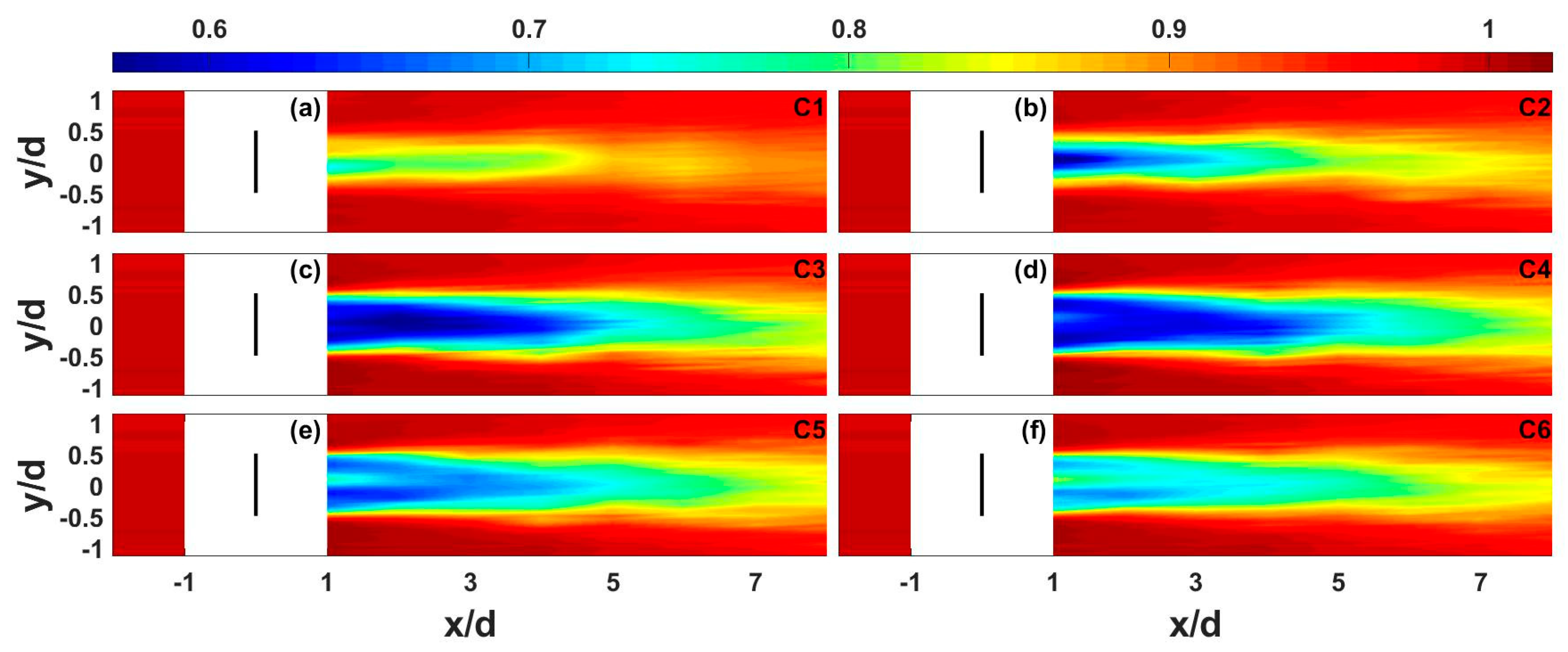
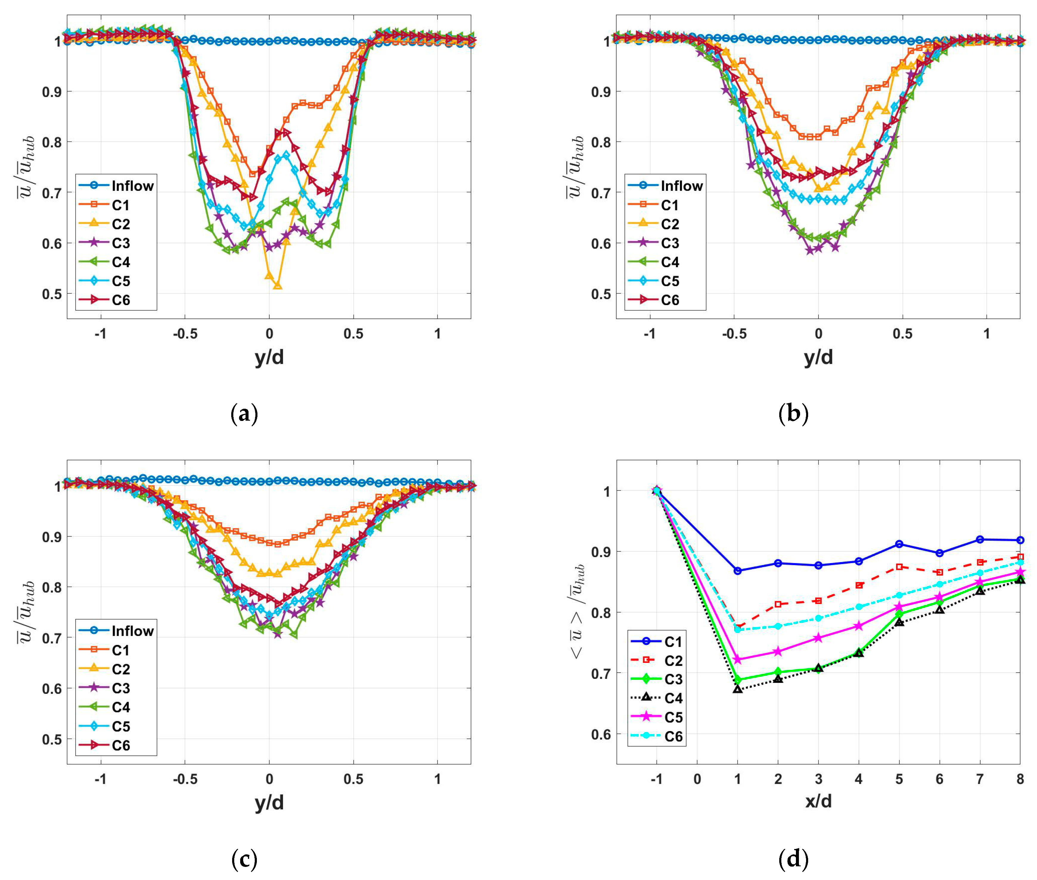
Figure 7 shows the contours of the time-averaged streamwise velocity in the hub-level horizontal plane for the turbine operating at the different TSR conditions. To further compare the wake-induced velocity deficits at the different TSRs,
Figure 8 shows the comparisons of the lateral profiles of the time-averaged streamwise velocity at the streamwise locations of x/d = 1, 3, and 5, as well as of the streamwise profiles of the mean velocity
. Here, the angle bracket
represents a laterally spatial averaging from y/d = −0.5 to 0.5. From the two figures, both the spatial distribution of the turbine wakes and the magnitude of the wake velocity deficits have changed significantly in different TSR conditions. Coincidentally with the maximum power coefficient C
p = 0.212 at the C4 condition, the turbine rotor operating at the TSR = 4.1 leads to the strongest turbine wake in terms of the spatial size of the wake (see
Figure 7) and its velocity reduction extent (see
Figure 8d). This result explains that, at this operation stage, the small turbine extracts the most fluid kinetic energy to achieve the maximum energy output and conversion efficiency and, therefore, produce the strongest turbine wake.
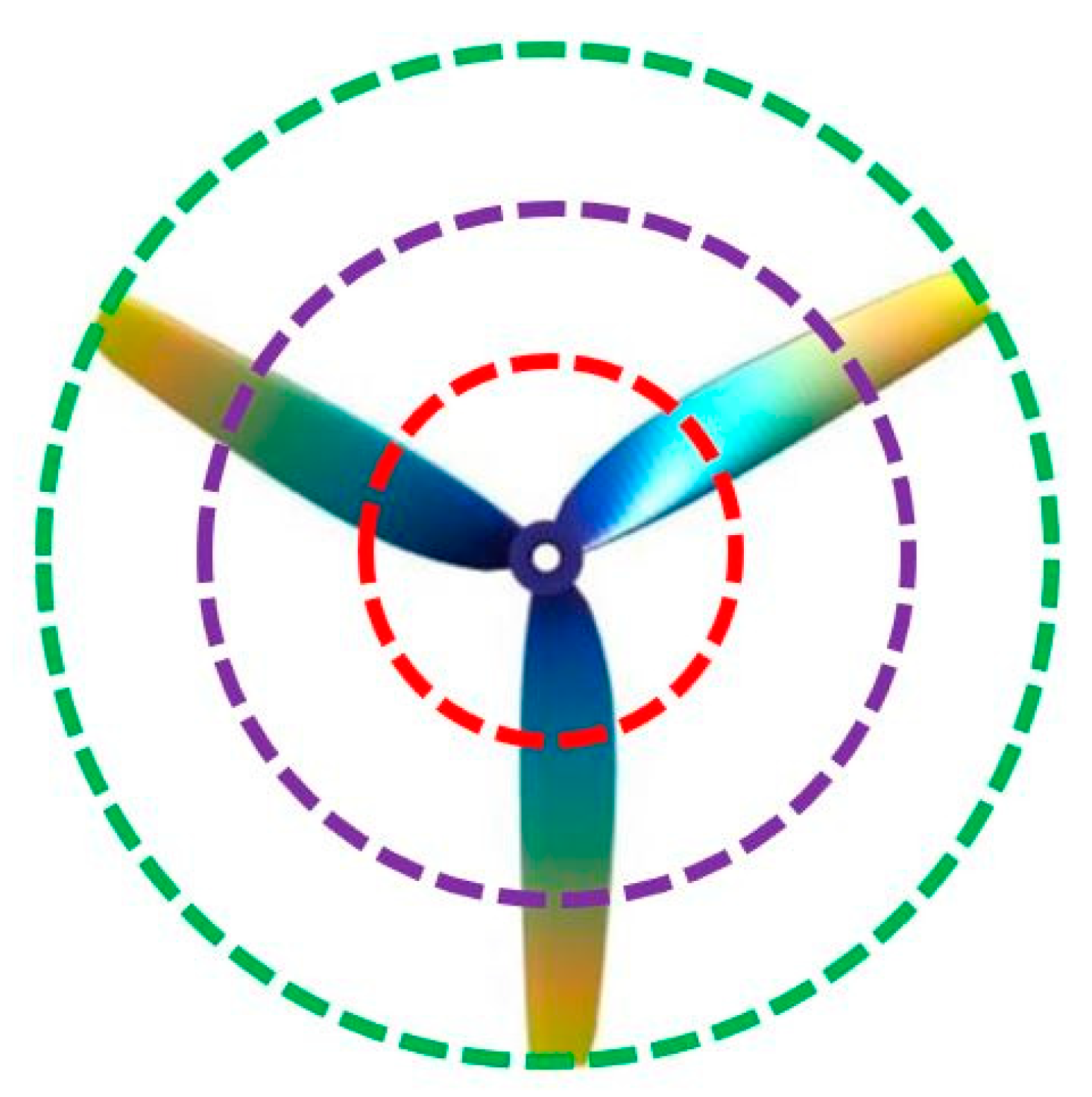
In the further discussion associated with the wake velocity distributions affected by the blade under the different TSR conditions, one can divide three equal parts along the radius and then split the rotor-swept area into three regions (i.e., inner circle, middle annulus, and outer annulus), as illustrated in
Figure 9. The changes in the wake velocity distributions (particularly in the three regions) under the different TSR conditions at the same streamwise location attracts considerable attention, especially the variability of the wake velocity distributions at x/d =1 (
Figure 8a). The turbines, operating at the C1 and C2 conditions, lead to the large velocity deficits in the inner region and small velocity deficits in the middle and outer areas (i.e., peripheral area). In particular, the turbine at the C2 condition produces a V-shaped wake velocity distribution, accompanying the local most significant velocity deficit in the wake center at x/d = 1. At the C5 and C6 conditions, the turbine produces large velocity deficits in the peripheral regions and small ones in the inner region, which is similar to an M-shaped distribution. Moreover, the turbine operating at the C3 and C4 conditions leads to the large velocity deficits among the three regions (i.e., inner, middle, and outer), with the occurrence of larger electromagnetic torque (as shown in
Figure 6c). In the six conditions, one can conclude that the large velocity deficits are associated with more incoming flow kinetic energy converted by the blades into mechanical energy to help drive the blade rotation and the generator shaft, and vice versa. This behavior, together with the mean velocity distributions (shown in
Figure 8d), can establish a significant relationship that a large torque will result in the generation of a strong turbine wake downstream. Hence, based on the results in
Figure 6,
Figure 7,
Figure 8 and
Figure 9, the turbine rotor at the C3 and C4 conditions generates larger torques (shown in
Figure 6c) and then causes the downstream wake losses to be much greater than the other operating conditions. These results indicate how the efficiency of the flow momentum extraction by the rotor changes with the blade angular velocity (as well as with the TSR).
Figure 10 shows the time-averaged vertical velocity contours in the hub-level horizontal plane for the turbine operating at different TSR conditions. Since the selected turbine rotor rotates clockwise (if one stands the upstream of the turbine) and induces wakes to rotate counter-clockwise, the vertical velocity distribution has the positive upward velocity at y/d < 0 and the negative downward velocity at y/d > 0. The magnitude of the vertical velocity is found to be larger at the C3 and C4 conditions where the rotor has larger torque generation and to be smaller at the C1 and C6 conditions, which have lower torque production. Therefore, the torque increment facilitates supplying inputs from the blade reaction force to raise the angular momentum of the wake flow and the vertical velocity magnitude. It should be pointed out that this behavior is different from the extraction of the flow momentum in the streamwise direction that leads to the velocity deficits in the wake.
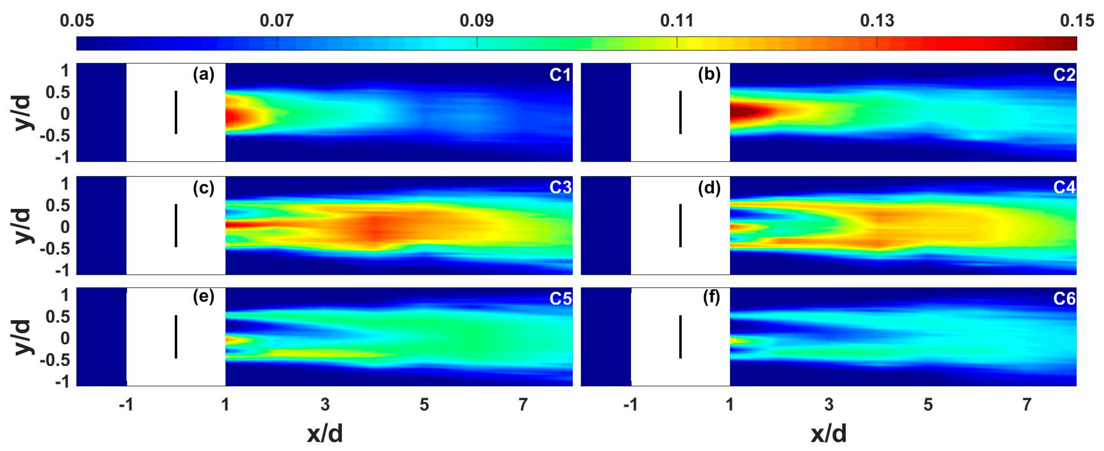
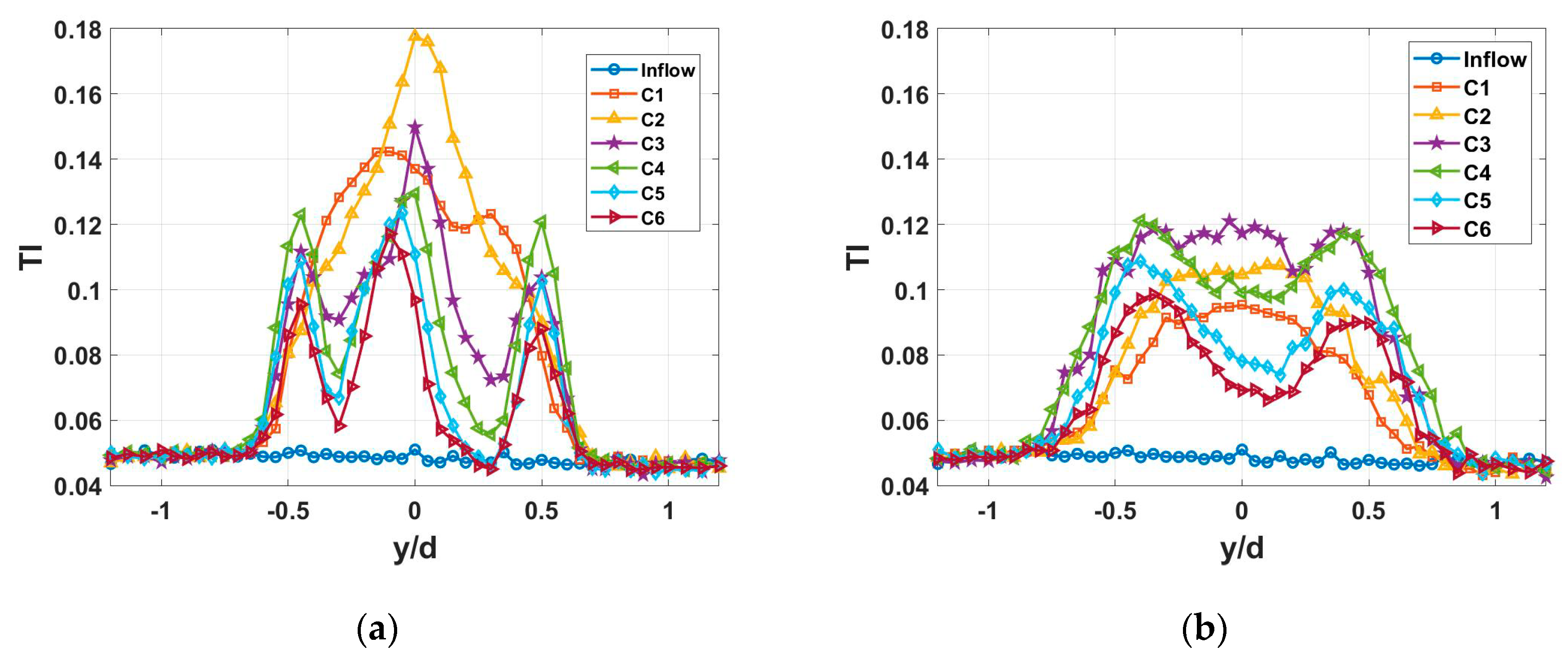
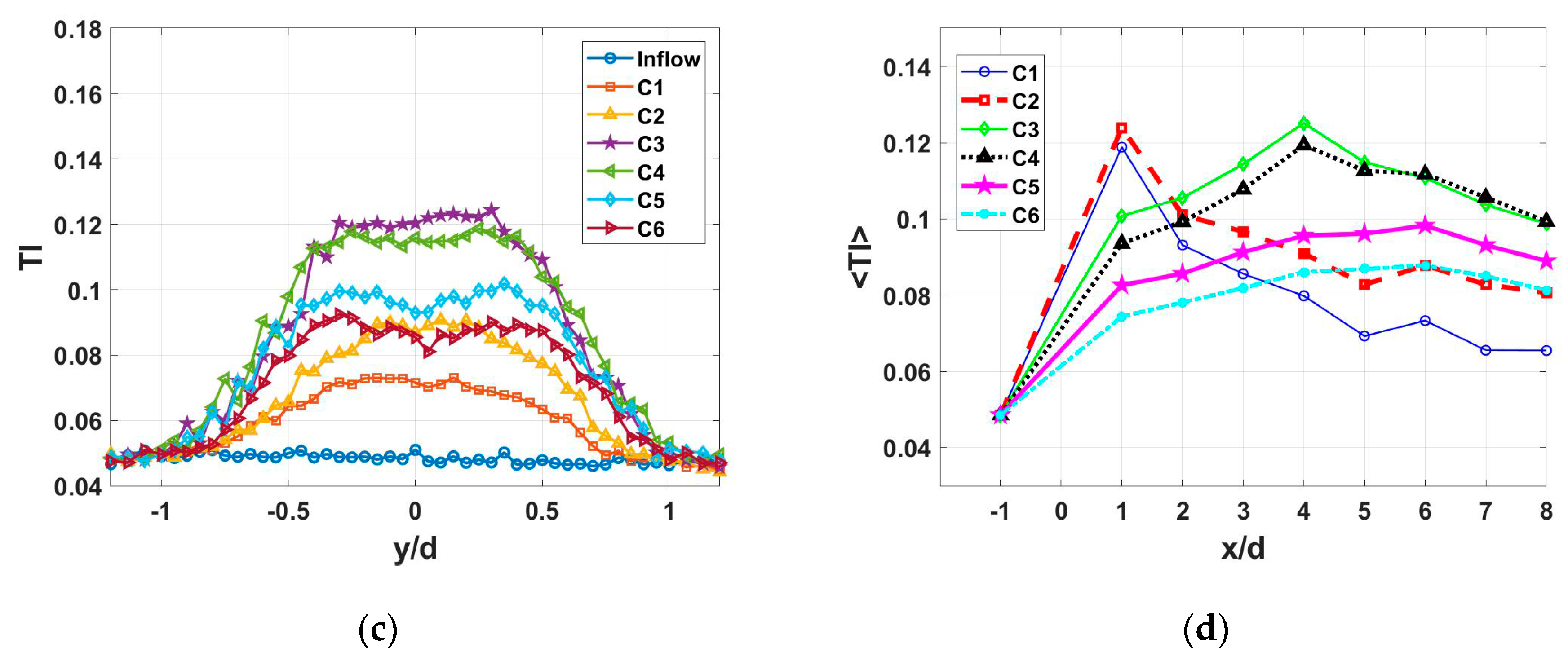
Figure 11 shows the total TI contours in the hub-level horizontal plane for the turbine operating at the six TSR conditions. To further compare the wake-enhanced TI at the different TSRs,
Figure 12 shows the comparisons of the lateral profiles of the total TI at the streamwise locations of x/d = 1, 3, and 5, as well as of the streamwise distributions of the mean TI, which is averaged laterally from y/d = −0.5 to 0.5. In the figures, the turbine rotor produces different TI distributions under the considered TSR conditions. The local maximum wake-induced TI is found about 0.18 and appears at x/d = 1 in the C2 condition, which is accompanied by the occurrence of the maximum wake deficit (as shown in
Figure 8a).
The generation of active wake-enhanced TI is observed in the rotor positions near the blade root (or the nacelle) and the blade tip. The maximum TI under each TSR condition occurs in the downstream locations where the wake turbulence induced from the nacelle and the blade tip merge at x/d= 1 to 2 in the C1 and C2 cases, x/d = 4 in the C3 and C4 cases, and x/d = 5 to 6 in the C5 and C6 cases. Hence, the position with the occurrence of the TI enhancement extends to a further downstream location with the TSR increment. Regarding the variability of the TI magnitude, the turbine at the C3 and C4 conditions produces an overall TI much higher than that at the other conditions. Within the turbine rotor, the enhanced TI near the blade tip becomes stronger with TSR increment in the C1–C4 conditions, whereas the TI near the root gradually weakens with TSR increment in the C2–C6 conditions. This result, together with the wake velocity, is shown in
Figure 7 and
Figure 8 where the presence of large wake velocity deficits leads to strong mean velocity gradients, which promote the generation of the active wake-enhanced TI. This behavior indicates that a certain segment of the blade effective for torque generation extends from the root position toward the blade tip position with the increase of the TSR.
In the six TSR conditions, the power outputs increase and then decrease with the increment of the blade rotating speeds (or TSRs), under which the magnitudes in the wake velocity deficits and the enhanced turbulence intensity show a similar trend of increasing first and then decreasing. The maximum power coefficient is found to appear on the turbine operating at the C4 condition (TSR = 4.1). Furthermore, the comparison of the TI magnitude at the C3 and C5 conditions reveals a remarkable difference, where the turbine at the C5 condition produces a larger power output and a turbine wake with a smaller TI magnitude compared with the turbine operating at the C3 condition. This result accounts for a larger power output of a wind turbine that can be achieved through the regulation with a higher blade angular velocity and a smaller shaft torque. Under this condition, the turbine-generated wake has lower velocity deficits and less TI enhancement, which is beneficial to the power production efficiency on the downstream turbines in a large wind farm.
Note that at the C2 condition both the mean streamwise velocity and the TI show a V shape distribution at x/d = 1, with the larger velocity deficit (also associated with larger wind shear) and stronger enhanced TI in the inner circle region. By coincidence, this behavior accounts for the rotor within the inner circle region at this operating condition extracting more momentum from the incoming flow and leads to the V-like wake velocity distribution and turbulence intensity distribution. The presence of larger wind shear in the wake facilitates strong turbulent mixing, which results in a U-like wake velocity distribution at the downstream locations of x/d = 3 and 5.
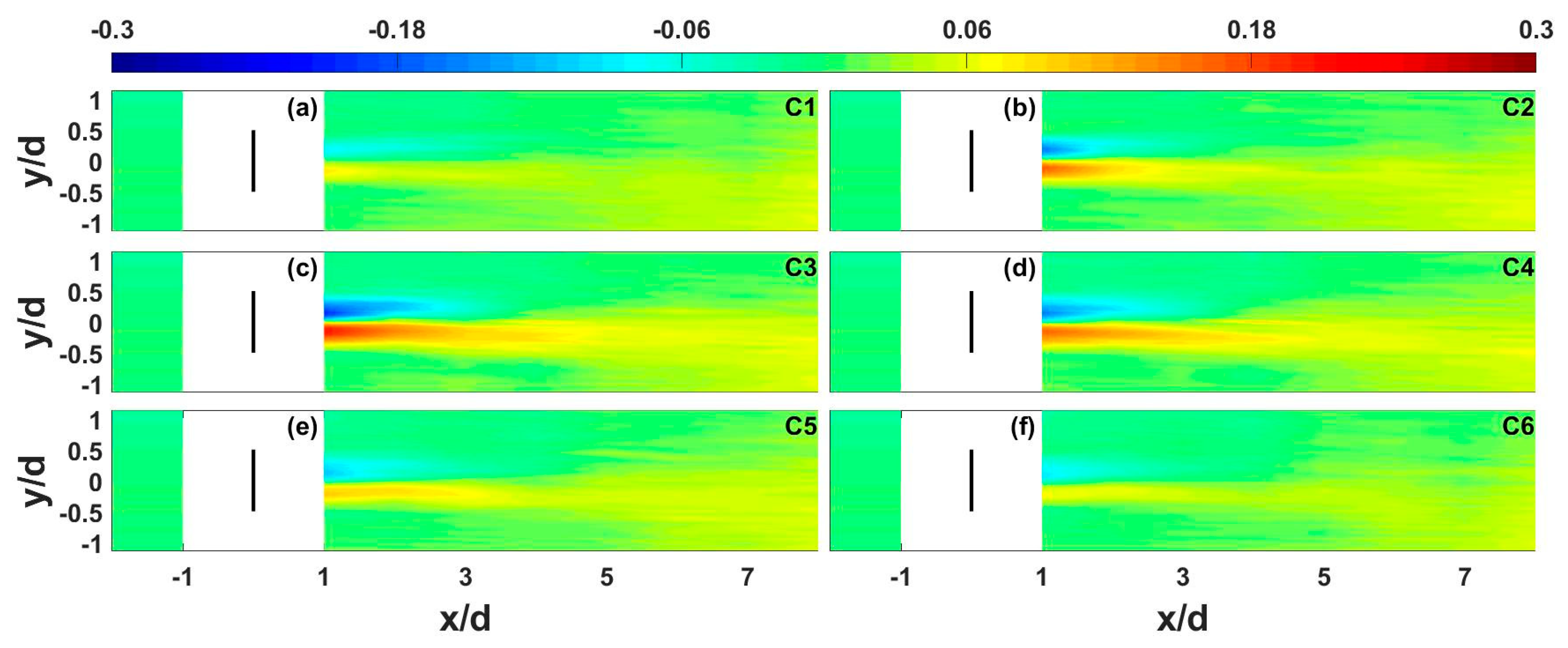
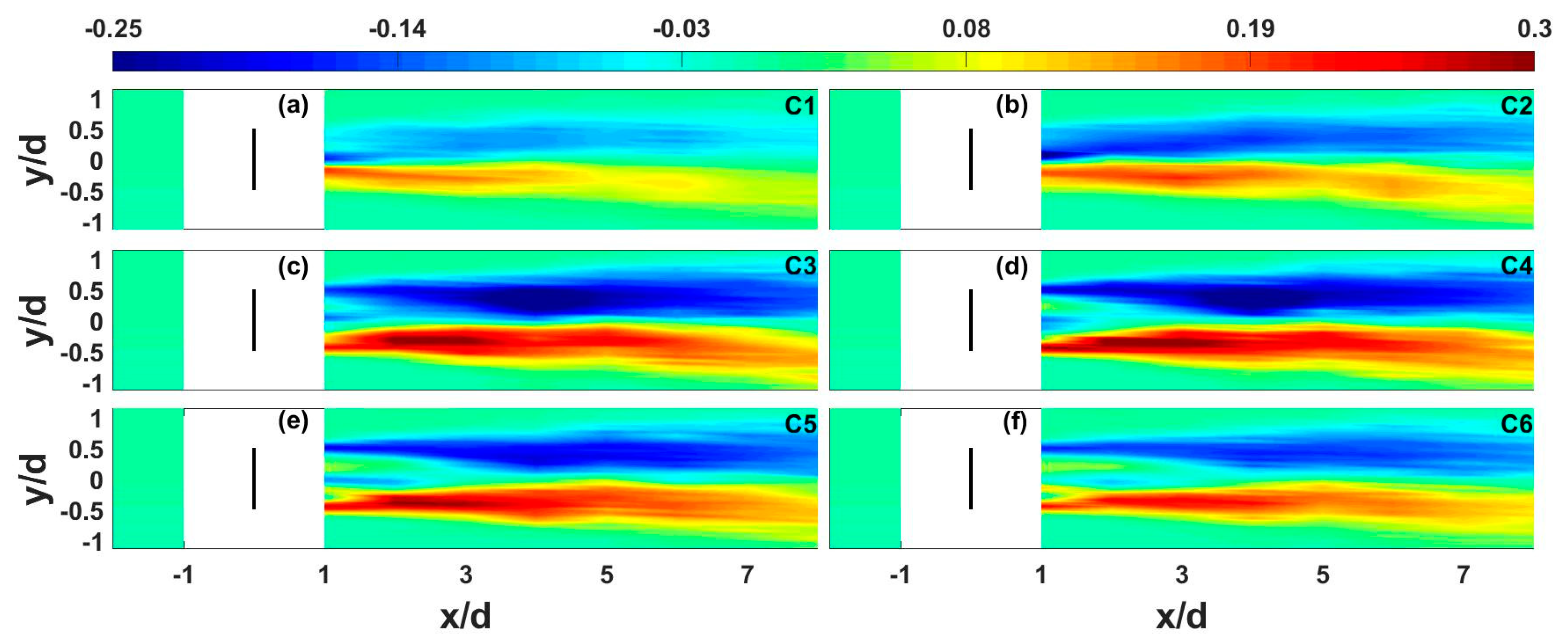
Figure 13 presents the contours of the lateral momentum flux in the hub-level horizontal plane for the turbine operating at the different TSR conditions. Here, the lateral momentum flux is computed from the covariance of the two instantaneous streamwise and spanwise velocity components as
where the overbar denotes temporal average,
is the lateral momentum flux, and
and
are instantaneous streamwise and spanwise velocity components, respectively. The magnitude of the momentum flux can be applied to explain the direction and extent of momentum transport in the turbine-induced wake area. As shown in
Figure 13, the positive and negative momentum fluxes represent the upward and downward fluxes (on the figure), respectively, to facilitate the momentum transfer inward to the turbine wakes. As shown in
Figure 7, the large wake velocity deficits appear on the turbine rotor operating at the C3 and C4 conditions, which are, of course, expected to require more momentum transported from adjacent flows to promote wake recovery. Hence, it can also be expected that increases in the magnitude of the lateral momentum flux in the wake region are relatively larger in the C3 and C4 conditions than the others. This behavior indicates that larger wake velocity deficits correspond to the stronger momentum fluxes.


