1. Introduction
In recent years, by providing safe, efficient and convenient transport services to a large number of passengers in a short period of time, metro systems are playing a more important role in modern transportation systems all over the world [
1]. It has been a common sense that urban rail transit systems have great advantages in enhancing the energy utilization efficiency over private cars and other public transportation modes, which enables a greener choice with higher environmental friendliness capabilities [
2,
3]. However, according to the fast development of the urban rail transit networks in many cities, the extended energy consumption reduction solution is becoming a big concern for both the research and rail operation fields. Energy efficient operation solutions are attracting more attention to optimize the system cost in the whole lifecycle, reduce carbon emissions and realize public environmental responsibilities.
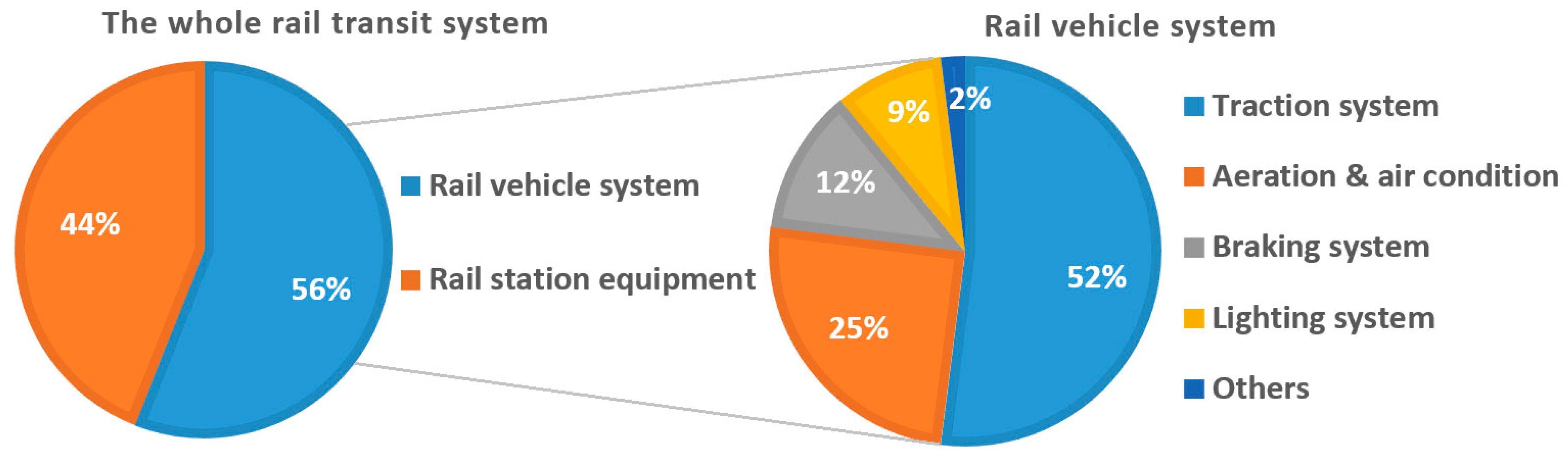
Among the different factors of energy consumption in the urban rail transit trains, including the train braking, lighting, aeration and air condition, the train traction plays the most significant role, which reaches about 52% of the total energy consumption of the train system in Beijing (see
Figure 1) [
4]. A collection of research works published in the 1990s begun to focus on optimal train control methods [
5,
6,
7,
8]. In recent years, great efforts have been made to develop advanced energy-efficient traction methods, which calculate and suggest energy-efficient driving strategies that are feasible with the permitted trip time schedule and track conditions, and do not require extra railway infrastructure investments. Many existing works in the literature concentrate on the calculation of energy-efficient train driving control strategies to effectively reduce tractive energy consumption under specific constraints, including the traveling time, running distance within adjacent rail stations, train traction/braking force characteristics, train parameters and the passenger distribution features, etc. The most typical solution for solving the condition-constrained tractive energy saving problem is an intelligent optimization approach, such as genetic algorithm [
9], particle swarm optimization [
10], simulated annealing [
11], differential evolution [
12], artificial bee colony method [
13], etc. Some of these methods have been validated with field experiences in design and optimization of the train’s driving curves for automatic train operation [
14,
15]. In addition, efforts also have been made to the analysis of the correlation between the energy efficient control and specific issues. Zhang et al. [
16] proposed the Comprehensive Evaluation Index (CEI) to analyze integrated optimization strategies of urban rail transport by calculating the traction energy cost and the technical operation time. Lin et al. [
17] realized the optimization of the train dwell time with a multiple train operation model for an energy conservation target. Tian et al. [
18] proposed a multi-train traction power network modelling method to determine the system energy flow of the rail system with regenerating braking trains. Hamid et al. [
19] explored how errors in train position data affect the overall energy consumption under a single train trajectory optimization scheme. Gomes et al. [
20] evaluated the potentials of the energy efficiency from “fixed block” to the “moving block” type using the empirical data and the statistical approaches. Zhou et al. [
21] take into account multiple issues in the energy minimization of the traction system, including train headway, interstation runtime, coasting on downhill slopes, and the variations of train mass due to the change of on-board passengers. Yang et al. [
22] further investigated the effect from multi-phase speed limits in optimizing the total energy consumption of a metro line using the optimization techniques.
Different from the abovementioned solutions for optimized driving control, the timetable, which describes the temporal-spatial constraints to the planned trains by defining the running time between two stations, has a direct and significant influence on the energy-efficiency of train operations. In recent years, the topic of energy-efficient timetabling has drawn the attention of researchers [
23]. Lv et al. [
24] proposed an energy-efficient timetable optimization method using a Mixed-Integer Non-Linear Programming (MINLP) model. Feng et al. [
25] developed a simulation- based approach to optimize both the timetable and control strategy considering the time margin that is caused by dynamically uncertain passenger demands in off-peak hours. Gupta et al. [
26] proposed a novel two-step linear optimization model for energy-efficient metro timetables and realized a significant reduction in the energy consumption (the worst case being 19.27%). Canca et al. [
27] formulated the timetable design problem as a passenger load-dependent optimization problem and presented an effective solution using the sequential MILP algorithm. Scheepmaker et al. [
28] designed a method to solve the energy efficient operation problem taking into account the desired robustness and the optimal distribution of the running time supplements. Nitisiri et al. [
29] developed a parallel multi-objective evolutionary algorithm with hybrid sampling and learning-based mutation to solve the train scheduling problem. To further investigate the rail timetable rescheduling problem, Yang et al. [
30] introduced the Deep Deterministic Policy Gradient (DDPG) algorithm over a conventional Q-learning strategy to realize the energy-aimed rescheduling by adjusting the cruising speed and dwelling time continuously. It can be found that energy consumption level of a given timetable is actually an inherent attribute. As a secondary timetable quality indicator, it can be adjusted through a fine-tuning operation to the basic timetable solution with certain time allowances. Therefore, the quantitative evaluation of the traction energy conservation capability would be a decisive issue to determine the direction and the concrete strategy to adjust the timetable in the fine-tuning process. Given a real-world timetable, the individual driving control strategy of each planned train can be deduced with the practical field conditions and parameters, where an appropriate traction energy consumption reduction solution can be directly utilized. However, the knowledge about energy conservation results obtained from the train-level operation deduction is not sufficient to enable the fine-tuning of a candidate timetable scheme. It is of great value to illustrate the correlation between the achievable energy conservation capability and the specific energy consumption influencing factors, e.g., the interstation speed, train operation strategy, passenger load rate, train formation and train routing scheme. There is a lack of the correlation analysis for the achievable traction energy conservation capability with a specific rail timetable scheme. Furthermore, a rapid development of advanced swarm intelligence optimization technology in recent years enables great opportunities to solve the energy conservation problems in rail transport. The Bacterial Foraging Optimization (BFO) algorithm is a new swarm intelligence optimization technique that possesses a series of advantages including insensitivity to initial values and parameter selection, strong robustness, simplicity, ease of implementation, parallel processing and global search [
31]. BFO has been applied in a wide range of optimization problems such as the energy forecasting [
32], expert energy management considering the uncertainty [
33], the imbalanced data classification [
34], and robotic cell scheduling [
35]. The advantages of BFO against conventional swarm intelligence approaches greatly encourages us to solve the problems in enhancing the train driving control profiles and evaluate the energy saving space of the train scheduling schemes.
In 2017, a National Key R&D Program was launched to evaluate and demonstrate novel energy- efficiency enhancing techniques in Batong Line of Beijing Metro. With a rail operation organization perspective, the traction energy conservation capability of the real-world timetables is evaluated. This paper provides a case study of Beijing Batong Line. The contribution of this paper is to describe the correlation between the timetable-based tractive energy conservation capability and typical influencing factors. An optimization-based solution of energy efficient train driving control is introduced, and the correlation between energy-efficient-driving-enabled energy saving capability and some timetable-related influencing factors (i.e. running speed and passenger load rate) covering all the planned trains is revealed through data fitting models and boundary identification. The test results can give the metro operators and decision makers the overview reference information to understand the optimization space of specific timetable schemes, which would help them to adjust and update the operation plans with the energy-efficiency improving purpose.
The rest of this paper is organized as follows: In
Section 2, the energy efficient control method and the corresponding calculating solution are presented. In
Section 3, the principle and procedures of the correlation boundary identification is described by using the strategies introduced in
Section 2.
Section 4 shows a case study in Beijing Batong Line using two typical timetable schemes in practical operation. A short discussion and the planned future works are provided in the final
Section 5.
2. Energy-efficient Train Driving Control Method
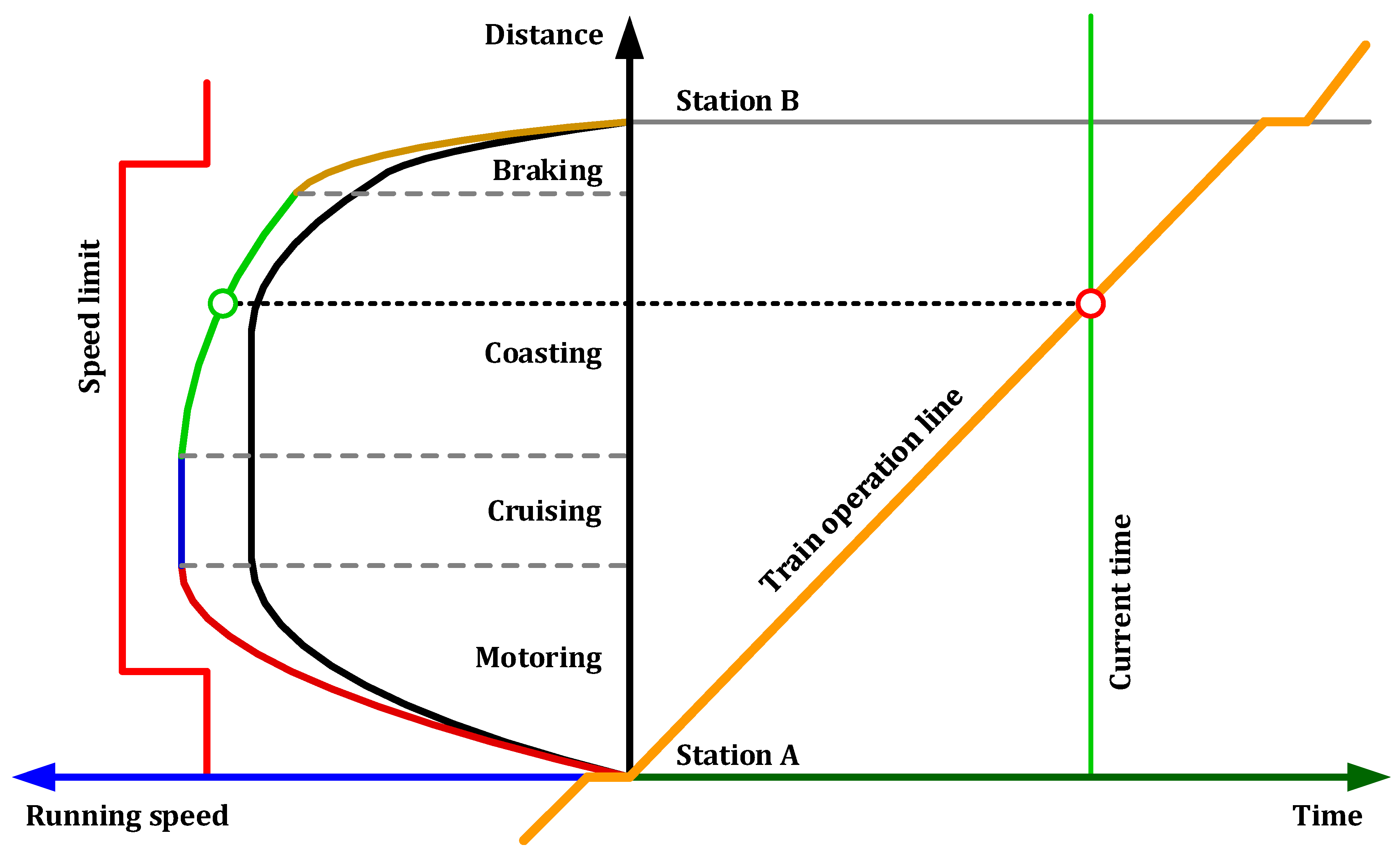
In order to evaluate the possible energy consumption level of the train traction system in field operation according to the time schedule, the key issue is to estimate the train operation profiles in practical operations, which will help us to find out the train driving control characteristics (see
Figure 2) and analyze the possible energy consumption by the traction system quantitatively.
The train kinematic modeling is the first step to derive the train operation profiles. As shown in
Figure 2, based on the general constraint from the time schedule, the practical moving operation of the train usually can be modeled using four typical movement modes. The driving status and the force condition under specific movement mode can be determined accordingly. Based on Newton’s second law of motion, the force for a moving train can be written as the following form:
where
M is the train mass,
st and
νt denote the time-varying running distance and the speed of the train at time
t,
F(
νt) and
W(
νt) indicate the traction force and resistance with respect to the running speed,
Rg is the force due to the gradient. When a train is operating in a specific movement mode, the force analysis can be performed accordingly based on the kinematic model in Equation (1), which can be summarized as follows:
(1) Motoring
The forward traction power is applied to accelerate the train against the resistance force, which raises the train speed until it reaches the required level to enable the following cruising operation. Therefore, all the elements in Equation (1), including the traction force F(νt), resistance W(νt) and the gradient force Rg, are involved in the description of the kinematics.
(2) Cruising
It is expected that the train keeps a constant running speed along the track. Therefore, traction force is provided as the sum of the resistance and gradient force, which means F(νt) = W(νt) + Rg. Due to the physical limitations of the traction system, a constant speed target cannot always be realized under time-varying moving conditions, and thus a fluctuation range (e.g., 2 km/h) for the cruising speed is suggested in field implementation.
(3) Coasting
The forward traction power is switched off in the coasting mode. The train will decelerate with the resistance and the gradient force, which means . Under the constraints of section length and the operation time TB from the timetable, the sufficient utilization of the coasting mode is one major approach to reduce the tractive energy since the movement of the train relies more on the inertia effect without consuming traction power.
(4) Braking
The backward braking force B(νt) will replace the forward traction force to decelerate the train, which means the Equation (1) will be written as .
It can be found that there would be different integration solutions of the above listed operation modes. As shown in
Figure 2, the black “speed-distance” curve represents an alternative which indicates a lower ratio of the coasting mode, where the temporal-spatial constraints by the timetable also can be fulfilled. In order to evaluate the energy conservation space and identify the boundaries, it is required to find specified energy efficient driving control solutions for all the planned trains in the timetable. Therefore, a calculation approach that is sufficiently effective in optimization and also computationally inexpensive is important for batch processing of a large amount of train plans.
2.1. BFO Algorithm
The Bacterial Foraging Optimization algorithm was proposed in [
36] based on the foraging behavior of
E. coli bacteria. The natural principle of the survival of the fittest illustrates that the natural selection will favor the bacteria with successful foraging strategies. The BFO algorithm was developed to realize the optimization capability by eliminating the bacteria with the poor fitness or reshaping them into good ones after a number of generations [
37]. By simulating basic movements of the bacteria, including the swimming and tumbling, the foraging behavior of the
E. coli can be utilized to establish the BFO architecture. The computational intelligence technique used in BFO is not affected by non-linearity and volume of the population. In the last few years, the BFO algorithm has been successfully applied to solve real-world engineering optimization problems [
38]. It has been pointed out that the BFO algorithm can reduce the global convergence, computational burden, time and also handle a number of objective functions [
39]. Comparisons with the conventional intelligent evolutionary computation algorithms, such as the Genetic Algorithm (GA) and Particle Swarm Optimization (PSO), have shown that BFO can realize a better optimization performance in many practical problems and real applications [
40,
41,
42]. Considering the advantages of BFO over the conventional measures, it is adopted in this paper to evaluate the energy-efficient capability of the timetables. The standard BFO architecture consists of four typical operations as follows [
43]:
(1) Chemotaxis
The swimming and tumbling movements are concerned in researching the behavior of bacteria. The swimming movement indicates moving within a pre-defined direction and tumbling means different directions can be selected during their entire lifetime. In the chemotaxis process, bacteria will perceive the level of nutrient content in the surrounding environment and thus guide the chemotaxis behavior. The generated unit length by tumbling will be used to define the direction of movement, which can be written as:
where
indicates the population of bacteria, the location of the
i-th bacterium at the
j-th chemotactic step, in the
k-th reproduction step and
m-th elimination and dispersal event,
C(
i,j) is the step size in a random direction, and
depicts a vector in the random direction whose elements lie in (−1,1).
(2) Swarming
When
E. coli bacteria find a nutrient rich environment, bacterial interactions with each other will encourage the accumulative effect at the high bacterial density area. By considering the swarming effect, the cost function
, which is also known as the nutrient function, will be denoted by:
where
is the cost function value to be added to the actual cost to be minimized to present a time varying cost function.
(3) Reproduction
In the reproduction process, the selected healthiest bacteria will live and the least healthy will die. According to the fitness value indicating whether an area is suitable for the bacteria survival, the bacteria in the place where the nutrients are rich will self-replicate, and they will be placed in the same location to keep a constant bacteria population.
(4) Elimination and dispersal
Gradual or sudden environmental changes for bacteria may happen due to different reasons. In order to prevent the premature or the local optimal solutions in the chemotaxis, the elimination and dispersal are necessary in the bacterial foraging. As the population-level long-term behavior, the elimination and dispersal events have possible positive effect on assisting the chemotaxis by placing the bacteria near the nutritious areas. The detailed theoretical derivations of the procedures for searching the global optimal solution can be found in [
36,
44].
2.2. Calculation of Energy-efficient Driving Control Solution
The track section between two rail stations is the fundamental unit for calculating the energy consumption level. It is usually divided into several sub-sections in generating the train operation profiles when considering the variation of track gradient and speed limit. Different from a detailed modeling to the traction control that is useful in analyzing the microscopic behaviors of the traction system [
45], all the types of driving control phases are considered during the whole trip in a section. For a sub-section, the suggested driving control solution consists of accelerating, cruising, coasting and braking according to the abovementioned kinematic model. In order to find an energy efficient train driving control solution, a state sequence is defined as
for the
nth sub-section, where
demotes the initial train speed in a sub-section,
represents the target cruising speed,
is the initial speed in the braking phase which is lower than
and represents the existence of the coasting operation,
is the final speed at the end of the sub-section. The values of the components in the state sequence are based on the speed limit of each sub-section and its neighborhoods. It means that the value space of a state sequence has to be collaboratively determined by the probable driving phases of its neighborhood sub-section(s), and that would be complicated under the long section cases with multiple changing points for the speed limit. The value of this state sequence directly determines the train operation profile, which provides a quantitative approach of carrying out the fine searching with the energy saving purpose.
By using the BFO algorithm, the energy efficient traction solution can be derived by an optimal train state sequences for all the sections. With the definition of the state sequence, it can be found that the multiple state sequences are taken as the variables need to be optimized for a planned train. The number of the variables is determined by the number of rail sections. With the derived results of state sequence, the speed values enable us to determine the control points for every control phase and draw the speed curves. The fitness of the bacterium is defined as the consumed traction energy by using the corresponding state sequence-based train speed profile. The amount of traction energy can be written as:
where
denotes the total journey time according to the derived state sequence, which should not exceed the planned time cost,
is the traction energy consumption in a time interval, and
represents the total number of time steps within the operation period of
.
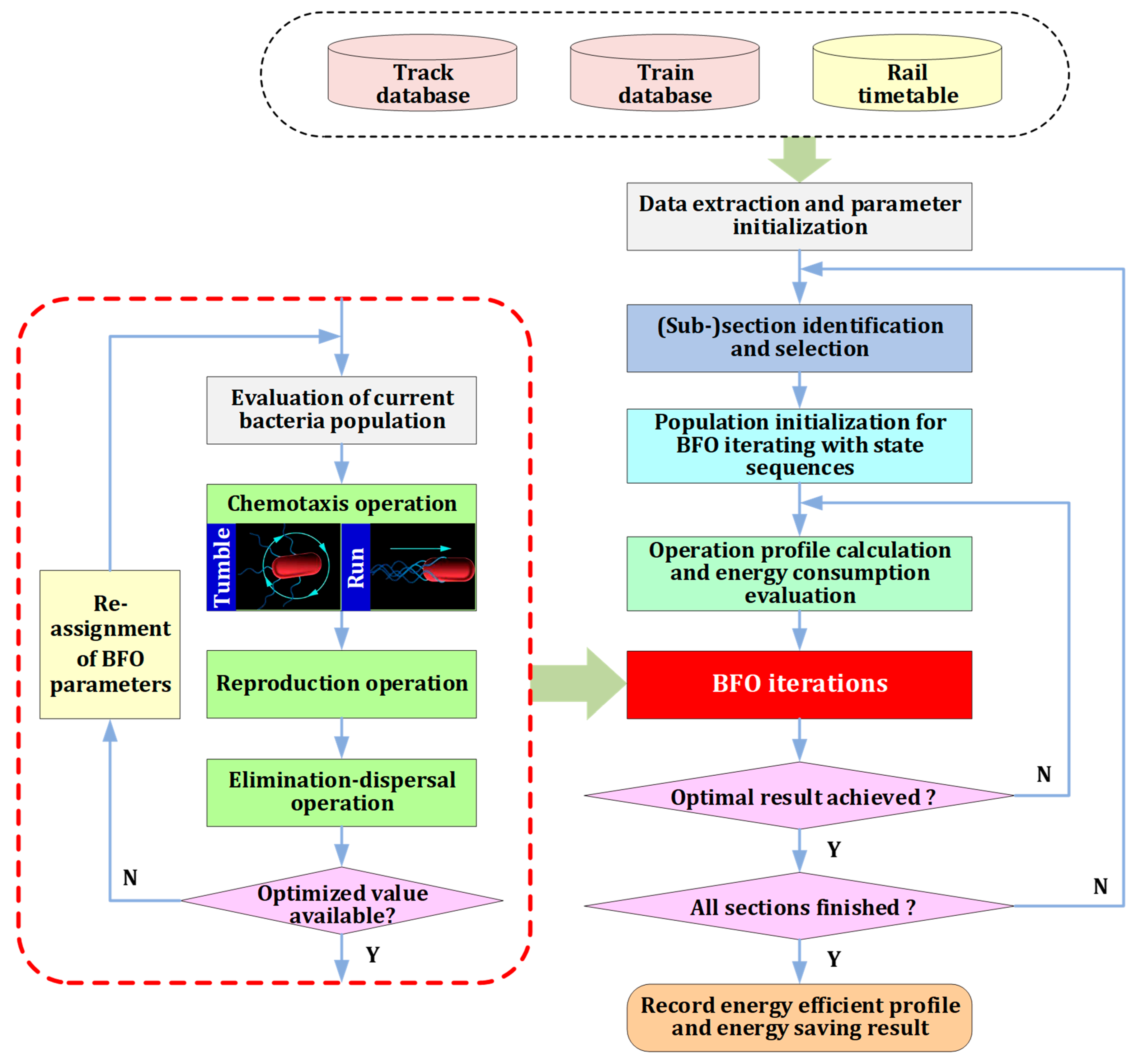
It can be found that the energy model depicted by Equation (4) only considers the traction and cruising operations. To derive the energy-conservation-oriented operation profiles and calculate consumed tractive energy, the BFO-enabled procedures can be described in
Figure 3. It has to be noticed that a simplified tractive energy calculation model is adopted in the presented solution compared to those consider detailed locomotive traction and train dynamics as [
46,
47]. Utilization of a detailed modeling solution will enhance the resolution of evaluation by integrating more realistic behaviors of the trains. Considering the fact that rail sections in the target line are not very long, we can use a relatively simple energy calculation model to guarantee the calculation efficiency of a timetable-based batch processing method. The model resolution enhancement for the energy consumption computation will be considered in our future research on integrated design of rail dispatching and driving control.
Figure 3 illustrates the framework of the energy efficient driving control solution calculation method using the BFO strategy. As shown in
Figure 3, the presented method mainly consists of two parts, including the offline database collection and online optimization. In the offline database collection process, information about the train, rail track and the timetable schemes is required to enable the following online calculation, and the correctness and accuracy of the database are significant to the creditability of the BFO-based results. Based on that, the online optimization will be carried out by performing the speed profile prediction and energy-saving-oriented optimization. By utilizing a population of the bacteria, which indicate a group of train state sequences for each section, the BFO operation will be carried out according to the abovementioned procedures. With the optimization result, the optimal energy efficient speed profile is derived and that is able to enable the analysis of the energy conservation characteristics.
It has to be noticed that the calculation of energy efficient traction solutions as
Figure 3 and the following boundary evaluation is based on the following assumptions according to the real-world operation properties:
- (1)
We consider the temporal constraints from the timetable by utilizing the indicated arrival and departure times at each station. The speed profile of each planned train is determined by BFO-based calculation under the safety and running time limitations.
- (2)
To simplify the solution procedure, a similar assumption as [
48] for the train’s driving phase sequence in each rail section has been made, where four sequential phases are involved as shown in
Figure 2, including motoring, cruising, coasting and braking.
- (3)
Some parameters in the energy consumption model and profile calculation, such as train’s weight, acceleration and braking characteristics, and the resistance, are considered as the constant values according to practical situations.
- (4)
The passenger load condition is considered as a constant, where several average passenger load values have been evaluated in this research according to the statistical result in real operations.
To solve the energy-saving optimization model min
ETRA subject to the motion equations in (1), some constraints have been considered as follows:
where
denotes the section length between the two adjacent stations A and B,
indicates the running speed at the location
,
is the speed limit,
represents the maximum value of the acceleration or deceleration,
and
denote the derived and the scheduled trip times, and
is the acceptable limit to the trip time error.
3. Boundary Identification Method for Timetable
3.1. Calculation of Energy Conservation Profiles for Multiple Planned Trains
With the presented BFO-based calculation solution for rail sections, it is possible to evaluate the energy-consumption features of all the planned trains in the timetable. This can be regarded as an extension of the train identity dimension. By integrating time schedule data for multiple trains that are planned with the similar movement in the same transit line, the same parameters are adopted to perform the BFO-based calculation. Some differences among different numbered trains in the timetable will be considered in the calculation, including station stop schedule plans, running speeds within the sections and the passenger flow distribution conditions. These factors are also regarded as the independent variables in deriving the energy conservation profiles and identifying corresponding boundaries of the traction energy conservation space with respect to the given timetable.
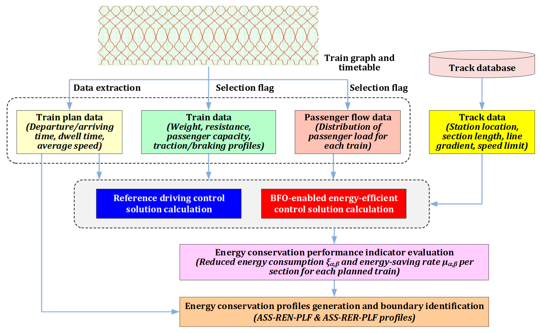
Figure 4 shows the flowchart of the energy conservation profile calculation method. The data of train, track and time schedules of multiple planned trains are taken as the inputs. With a specific input and parameter configuration, the unique energy efficient operation solution for each train plan can be obtained, with which the optimized train movement can be described by speed-distance curve and speed-time curve respectively. For the evaluation purpose, reference train operation profiles are also computed in parallel. The fully consistent assumptions and constraints for deriving the BFO-enabled solution as stated in
Section 2.2 are adopted in the calculation of reference profiles. The coasting phase is also involved in the derived profiles according to the practice of driving control in the target line. A fixed deviation limit to the cruising speed and initial speed of the braking phase is adopted to derive the distribution of the driving phases. The major difference between the optimized and the reference solution is the utilization of the iterative optimization logic. The reference solution only uses the basic train traction calculation to generate the driving control profiles without an optimization process.
When we use
to represent the BFO-derived tractive energy consumption in the
β-th section for the
α-th train plan, the reduced energy consumption
against the reference profile is:
where the superscript ‘Ref’ corresponds to the reference solution-based result.
Based on that, the energy saving rate for each train at all the sections can be obtained by (11):
Thus, the saved energy and energy saving rate can be applied to generate energy conservation profiles. These profiles can realize the description of the correlation with independent variables, especially the interstation speed which fully reflects the dynamic characteristic of the trains under the timetable scheme. The acquirable energy conservation profiles are summarized as follows:
(1) ASS-REN-PLF profile
It describes the relationship between Average Section Speed (ASS) and Reduced Energy (REN) against the reference solution, under a specific Passenger Load Factor (PLF). The profile is represented by a series feature points , where indicates the average speed in the β-th section for the α-th train plan, and represents the amount of passengers per train.
(2) ASS-RER-PLF profile
Similar to the ASS-REN-PLF profile, the ASS-RER-PLF profile describes the relationship between the average interstation speed and the Reduced Energy Rate (RER) against a reference solution. Thus, a feature point in this profile can be represented by .
3.2. Boundary Identification Method
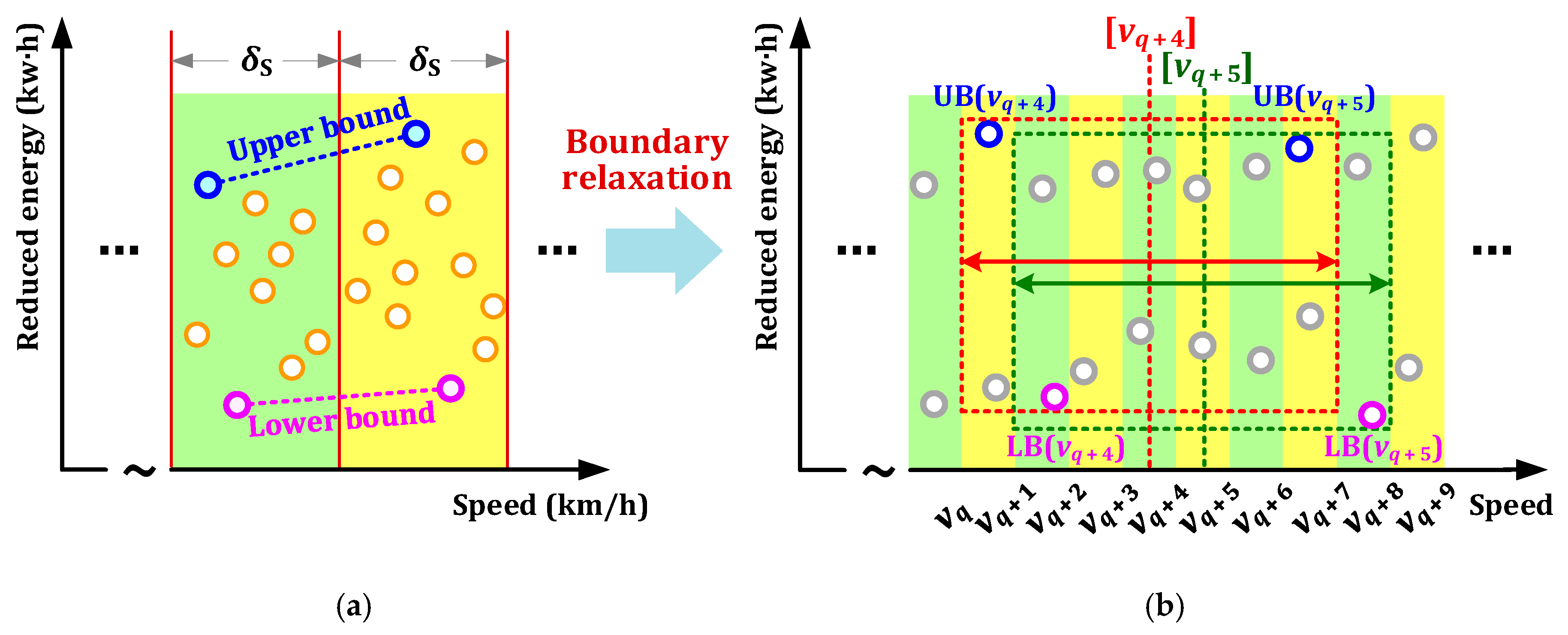
With the knowledge of the energy conservation profiles, the curve fitting approach is capable of establishing the numerical models of different factors. Besides that, it would be necessary to identify the upper and lower boundaries with the obtained feature point sets. The boundaries, especially the upper bound, bring the users the reference information to determine the way to evaluate the timetable schemes. In some existing applications, several strategies have been developed to realize an analytical determination of the boundaries of a given data set, e.g., the simple polynomial-based boundary fitting and the adaptive spline-based smooth boundary fitting. However, the existing examples aim to reach an analytical form of the “smooth” boundary by tolerating the residual error between the fitted values and the truth, which may not be acceptable for the capability evaluation case concerned in this paper. In order to derive tight boundaries for the acquired energy conservation profiles, a specific boundary identification strategy is proposed in this research using a piecewise detection strategy.
Taking the ASS-REN-PLF profile as an example, the piecewise detection is carried out in a series of speed intervals with a fixed piece width
. That means the whole value space of the interstation speed is divided into a number of pieces, and boundary identification will be carried out piecewisely. The value of
illustrates the resolution of the derived boundaries. The principle of identifying the upper and lower boundaries are described in
Figure 5.
As shown in
Figure 5, in the
j-th speed section, there would be multiple feature points
describing the relationship between the average interstation speed and the reduced traction energy. By extracting the maximum and minimum values, the boundaries will be:
where
and
are the upper and lower bounds,
represents the speed value of the boundaries in the
j-th sections,
indicates the number of the feature points fall in the
j-th sections, and
denotes the total number of the divided sections.
It can be found that a small value for
is strongly suggested since a higher resolution makes it possible to track the characteristics of the boundaries precisely. To avoid possible acute or frequent changes in the derived boundaries, a further boundary relaxation strategy is proposed to refine the original results by enhancing their smoothness. For a certain speed piece, a sliding window with a fixed width
is adopted to find a candidate boundary ensemble and extract the representative characteristics of the boundaries. Thus, the upper or lower bound with respect to a specific
would not be determined only by the feature points in the
q-th piece. Instead, a set of candidate boundaries
are used to identify the refined boundary values, where
. As seen in the example in
Figure 5, the candidate sets
and
are collected to generate the refined results for the
-th and the
-th speed section. Therefore, the final output of the boundaries are:
The procedures of the proposed boundary identification method are summarized in
Table 1.
With the above procedures, all the profiles can be examined and the corresponding boundaries can be obtained. The derived data sets will be given to the users to evaluate or even enhance the time schedule by using the quantitative results of the traction energy conservation capability.
4. Case Study
In this section, case studies for Beijing Metro Batong Line with both the weekday and weekend timetables are employed to illustrate the effectiveness of the presented energy efficient train traction solution and the boundary identification method for energy conservation capability evaluation.
4.1. Data Preparation
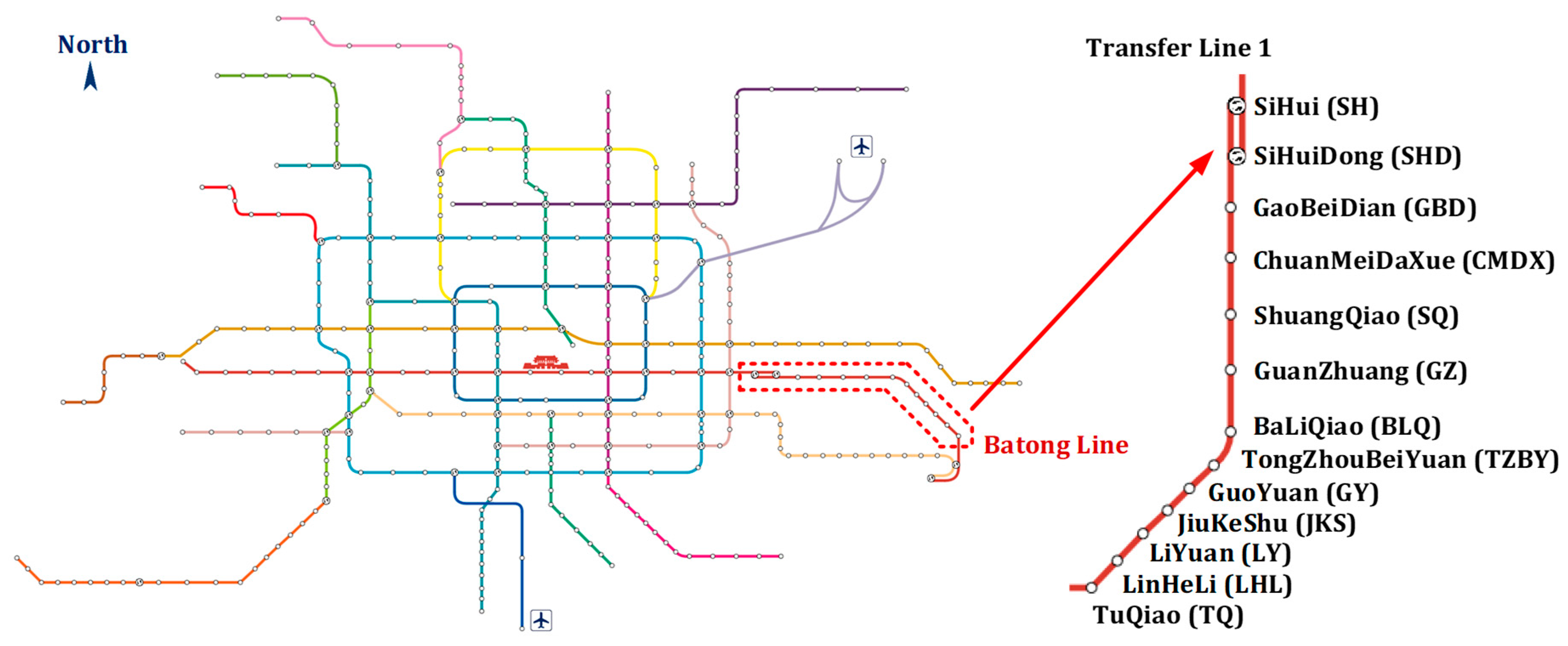
The Beijing Metro Batong Line is 18.96 km long with 13 stations. The southern extension section with 2 additional stations is not considered in this study. This line connects the central city of Beijing and the Tongzhou district, which is the sub-center of this city (see
Figure 6).
Table 2 shows the basic information of trains servicing in Batong Line. The resistance coefficients are defined as the technical document to identify the resistance force as the following formula:
where
Wm and
Wt are total weights of the motor unit and trailer unit, and
Nmt is the total unit number.
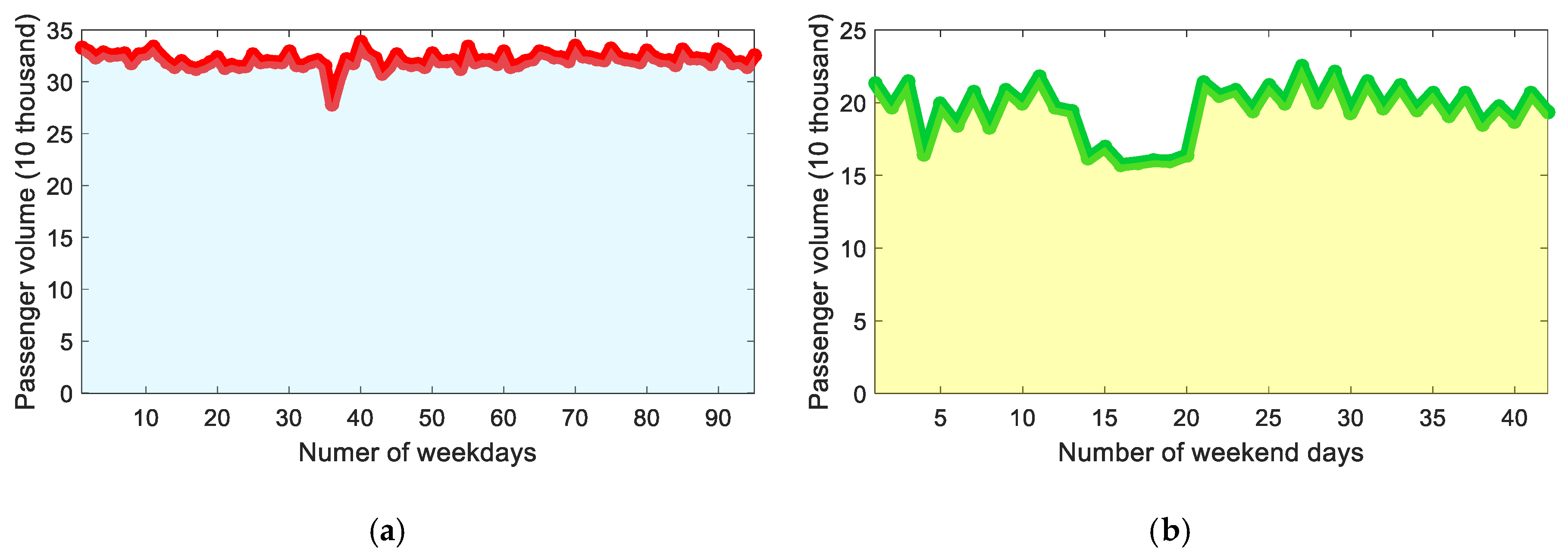
According to different passenger flow distribution features, two timetable schemes are adopted for weekday and weekend. A whole weekday timetable (5:00~24:00) of the Batong Line contains 438 planned trains, which indicates 219 trains in each direction. For the weekend version, there are 380 planned trains, where 190 trains are scheduled in each direction. From peak hour train graphs and the statistics of planned trains, it can be found that there are obvious differences in the passenger flow prediction and train management in weekdays and weekend days from the operator.
As one major factor that would influence the traction energy consumption level, the passenger load of Batong Line is also investigated in this case study. Statistical report about the daily passenger volume are collected from the operator when the two train graphs are utilized in practical operation.
Figure 7 shows the reported results of passenger volume in both weekdays and weekend days during a period over 4 months. It is obvious that the passenger load in weekend days is much lower than that in the weekdays, and that is consistent with the train operation plan arrangements.
By using true train parameters and track profiles of Batong Line, the following calculation and analyzes are performed to reflect the practically achievable energy conservation space of the given timetable schemes.
Based on the prepared data sets, the energy efficient train driving control profile calculation and boundary identification are performed and the results are given in the following sections.
4.2. Energy Efficiency Improved by BFO-based Solution
We firstly investigate the performance of the proposed BFO-based energy calculation solution for energy efficient train driving control solutions. A typical passenger load value is selected within the statistical results to enable the optimization calculation. For the derivation of energy efficient driving control solutions under the given timetable information, an average load condition of 738 passengers per train is adopted in the evaluation of the weekday timetable, and the typical average value of 525 passengers per train is utilized for the weekend timetable case. Results can be found in the following
Figure 8 and
Figure 9.
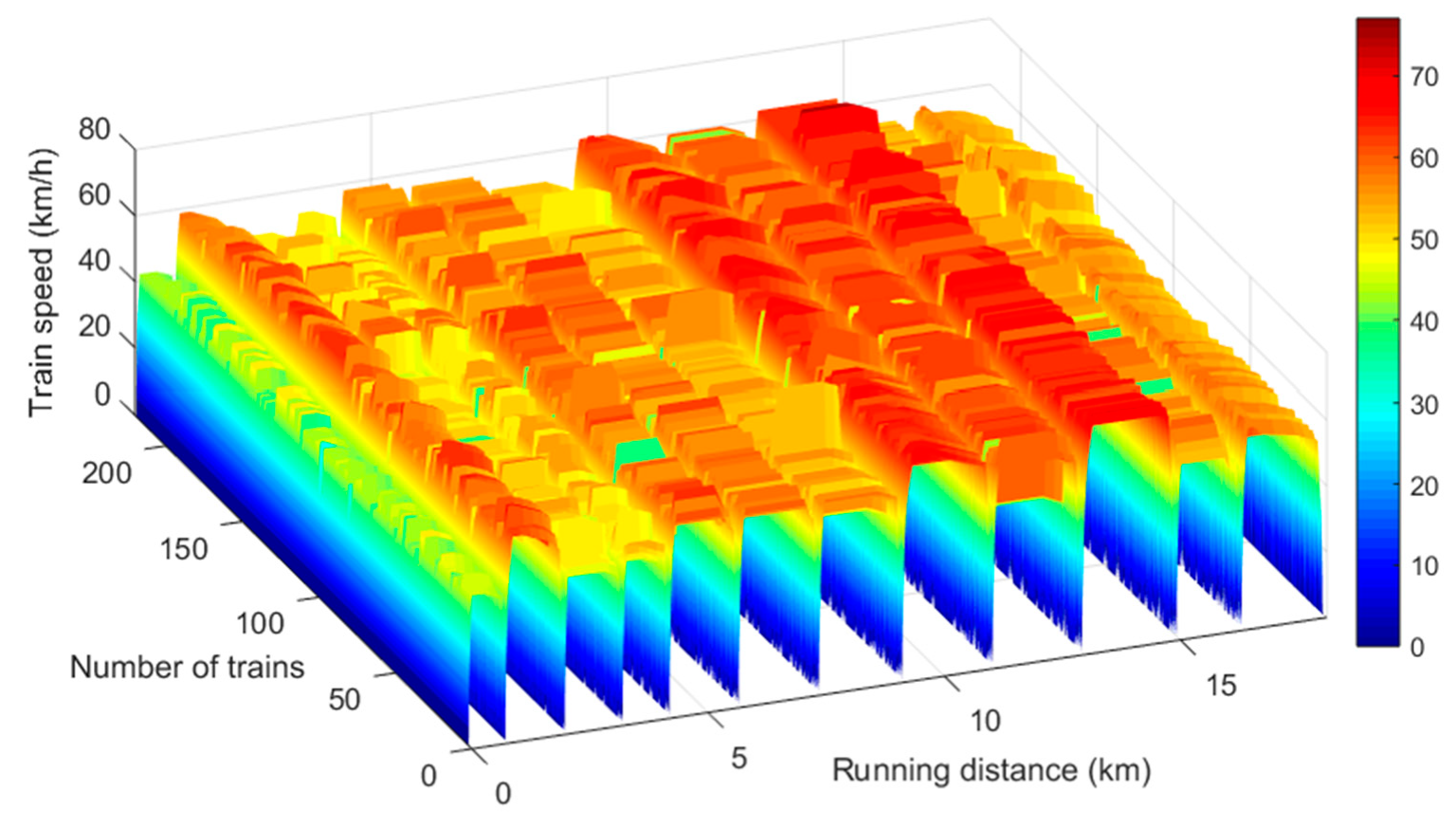
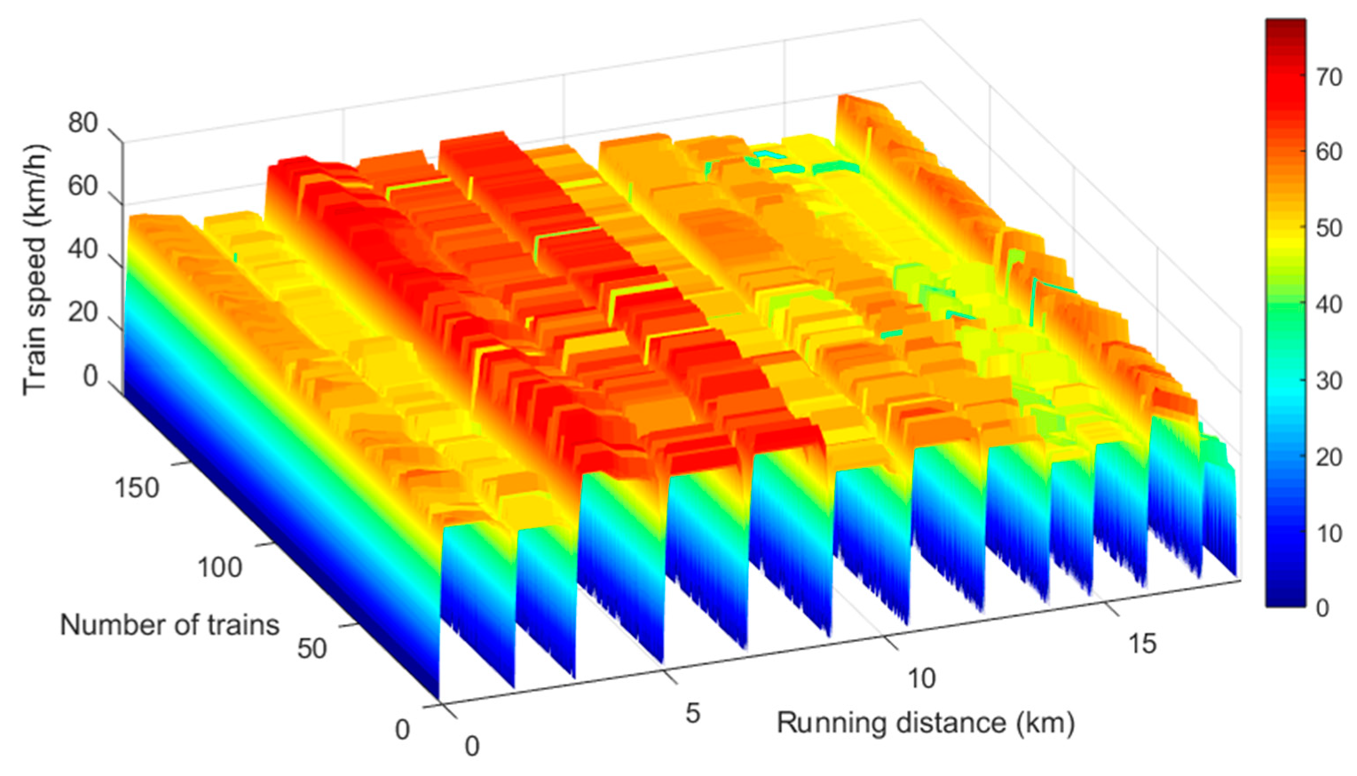
Figure 8 shows the derived train speed profiles in the TQ-SH direction by using the presented BFO-based energy efficient driving control solution with the weekday timetable. Speed-distance curves covering all 438 planned train in both the SH-TQ and TQ-SH directions have been calculated, from which it can be easily found that the energy efficient operation solutions of different trains by BFO iterations, even in the same track section, vary obviously with each other. Similarly, all the 390 planned trains in both directions with the weekend timetable have been evaluated, and
Figure 9 depicts the optimized speed profiles in the SH-TQ direction. At the same time, the reference driving control solutions for all trains in the weekday and weekend timetables are also calculated and compared with the optimized results.
Table 3 summaries the energy conservation performance of the BFO-derived operation speed profiles over the calculated references, where
Np represents the adopted average passenger load condition per train, Δ
ESec indicates the saved energy consumption per section against the reference solution-based results, and ‘Δ
ESec rate’ denotes the energy saving rate against the referencing results. To illustrate the performance differences for the trains, the train-level indices are also computed and summarized as shown in
Table 4, where Δ
ETrain is used to represent the reduced energy consumption for a planned train during the whole trip, and thus ‘Δ
ETrain rate’ indicates the train-level energy saving rate considering all the 12 sections. Statistical results of energy consumption level for the reference profiles are also given in these tables, where Δ
ESec-Ref and Δ
ETrain-Ref denote the tractive energy per section and the train-level energy consumption by the reference solution.
From these results, it can be found that the proposed energy efficient control solution calculation method using the BFO strategy is capable of reducing the tractive energy consumption in all sections against the conventional traction computation results. For the comparison about the amount of energy reduction at both the section-level and train-level, it can be found that the weekday timetable holds an advanced energy saving capability than the weekend timetable. This situation may be resulted by the difference in the passenger load rate in weekdays and weekend days. A relatively higher passenger load in the weekdays will increase the total mass of the trains and raise the used energy by the train traction system. With the same energy efficient driving control solution derived by the BFO technique, the absolute value of the energy reduction would be greater than the lower passenger volume case for the weekend days. However, the weekend timetable realizes a better energy saving rate, which takes advantage of the smaller absolute value of the section-level and train-level energy consumption.
Overall, the proposed method for calculating the energy efficient driving control solution based on BFO is able to save the tractive energy consumption under a given time schedule scheme. With the same configuration, quantitative evaluation of the energy saving performance against the referencing solutions can be performed, and that makes it possible of realizing additional analyses on the different influencing factors for the timetables and detecting the boundaries of specific profiles. The following sections will address the issue of boundary identification according to the proposed solution.
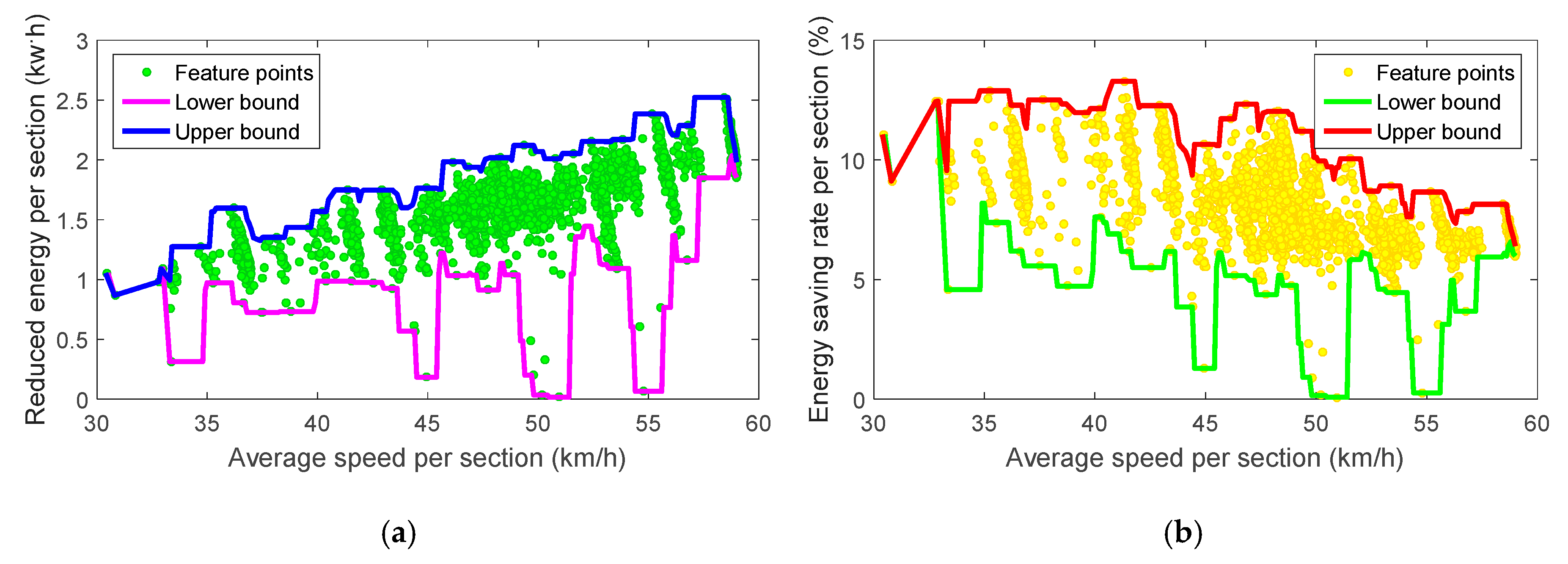
4.3. Boundary Identification of Speed-oriented Energy Conservation Profiles
The energy conservation profiles for two timetables are established by collecting the feature point sets. In this section, speed-oriented profiles are firstly concerned to illustrate the relationship between the energy efficient performance and the average section speed according to the train schedule plans. This section illustrates the boundary identification results for the ASS-REN-PLF and ASS-RER-PLF profiles under the weekday timetable. The piece width for boundary detection is set as
, and a window width of
is taken in the boundary relaxation. In order to depict the differences due to the passenger volume condition, two typical values of the average passenger volume per train, including
Np = 635 (minimum) and
Np = 773 (maximum), are used to carry out the presented boundary detection and relaxation strategies. Representative results are given in the following figures.
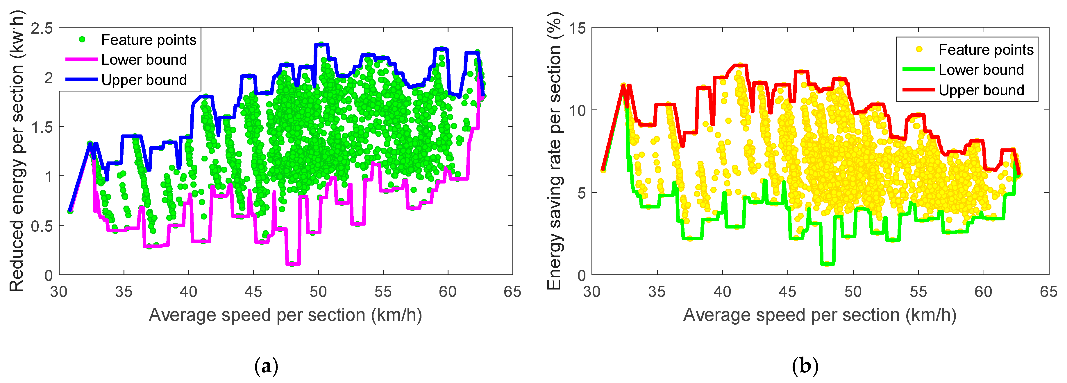
Figure 10 shows the boundaries in the SH-TQ plans under the condition
Np = 635. The results from the TQ-SH direction is given in
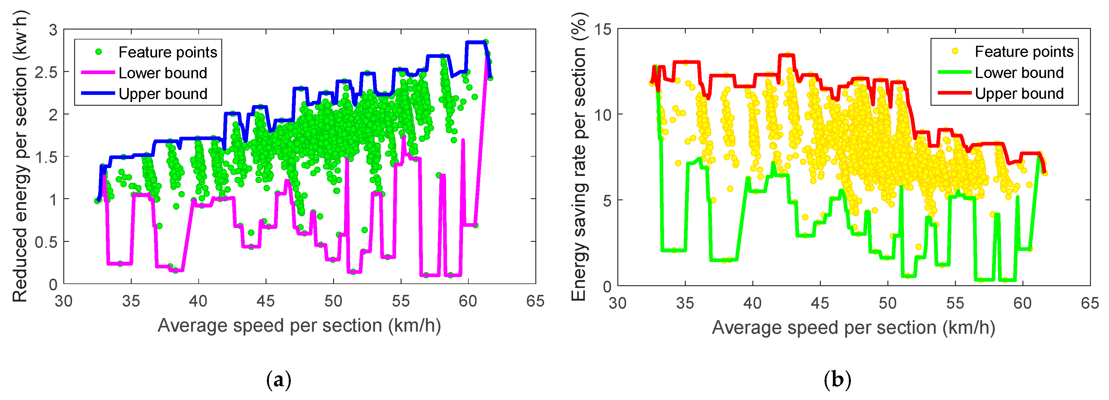
Figure 11 with
Np = 773. Similarly, boundaries under the given weekend timetable in both directions are shown in
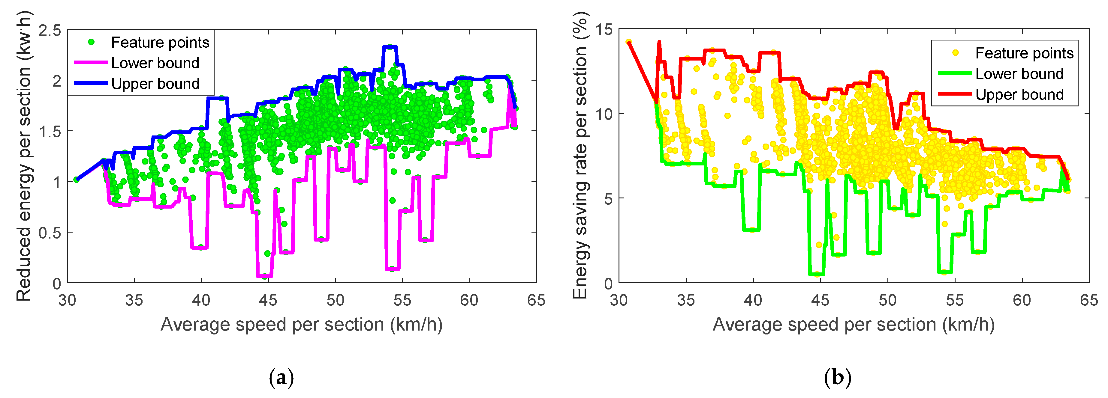
Figure 12 and
Figure 13, where the minimum (
Np = 414) and maximum (
Np = 593) passenger volume values from the statistical report in those weekend days are adopted.
From the derived results of the boundaries, it can be found that there is obvious difference in the general relationships with the reduced energy consumption and the energy saving rate. In both the SH-TQ and TQ-SH directions, the reduced energy consumption tends to increase with a larger section speed level. An enhanced upper bound reveals that the potential energy conservation capability of the timetable using the energy efficient driving control solution would be proportional to the corresponding average interstation speed. However, the boundaries of energy saving rate-related profiles behave differently. With the growth of average interstation speed, the achievable energy saving rate by BFO optimized train driving control solution tends to decrease gradually. Based on the investigation to the boundaries, it can be concluded that an increased average speed in the rail sections is surely suggested. At the same time, one has to be clearly aware of the constraint in the achieved energy saving efficiency. When tuning the running speed configuration of a timetable scheme, multiple factors and constraint conditions have to be considered with the energy-saving-oriented recommendations.
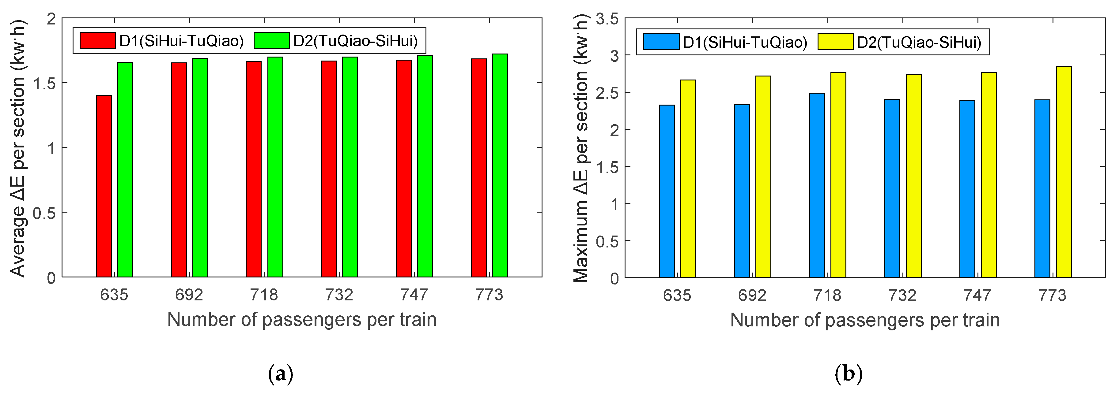
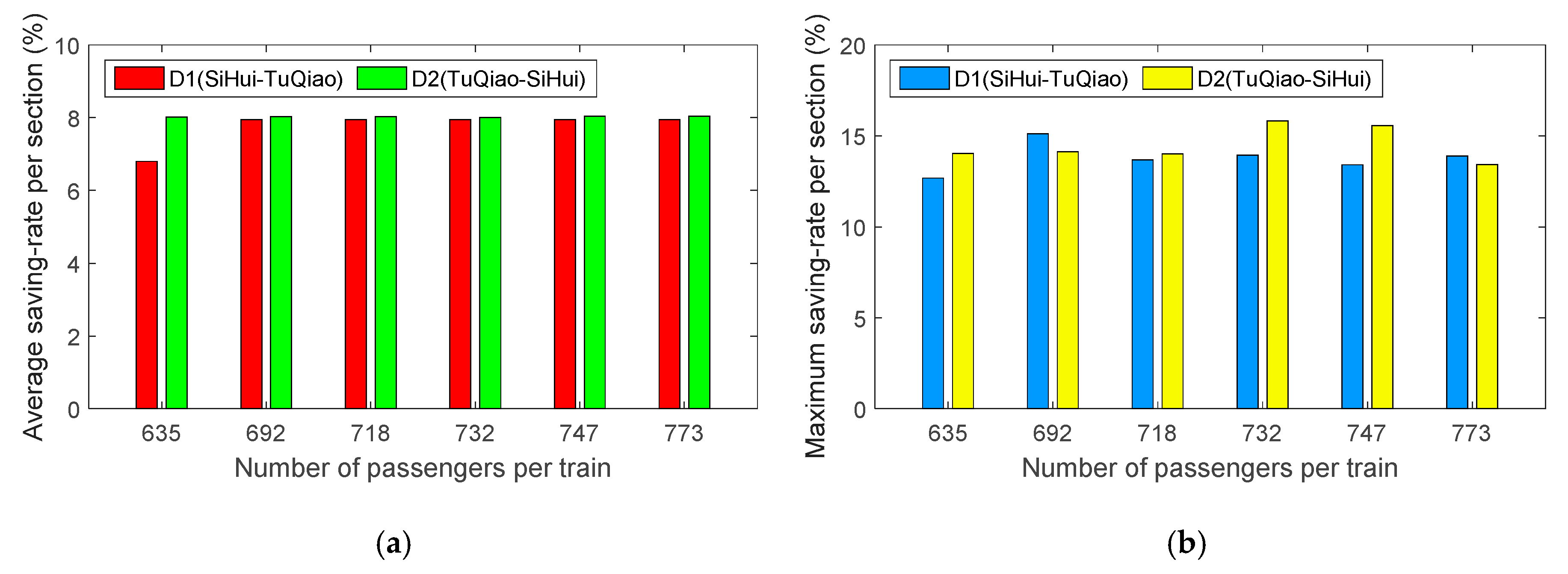
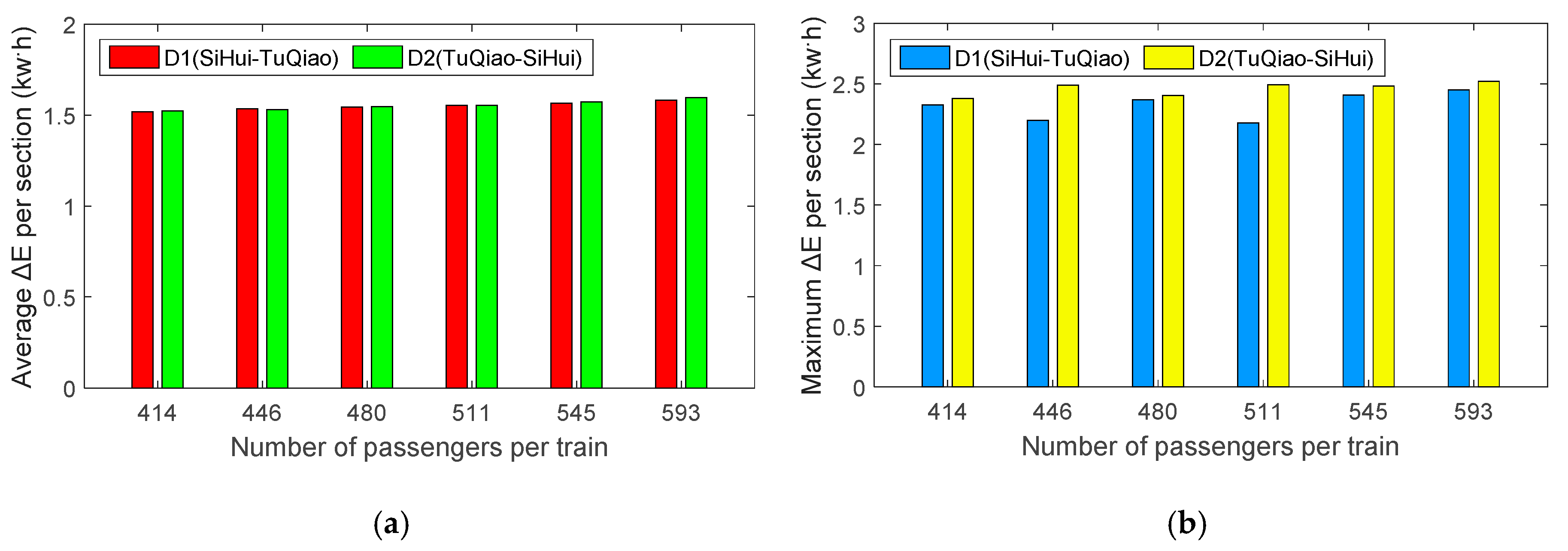
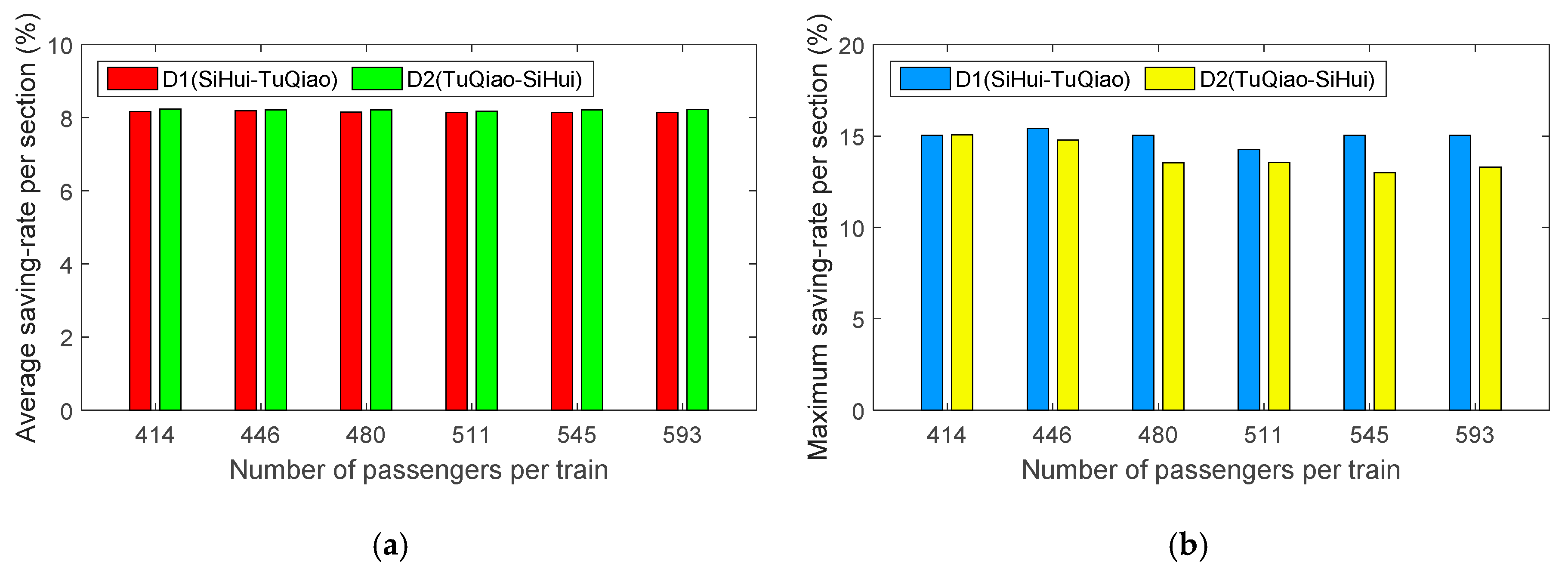
4.4. Analysis on Passenger Load Factor
From the boundary identification results mainly consider the effect from average running speed, some preliminary knowledge results have been acquired to assist the evaluation of a specific timetable scheme. In order to further discuss on the correlation among the energy efficient driving control, the train speed parameter and the probable passenger load conditions, more passenger volume samples participate in the analysis to demonstrate the effect from the passenger flow features. Six additional passenger volume values are sampled from the statistics as shown in
Figure 8 to enrich the data set for both the two timetables, which means {635, 692, 718, 732, 747, 773} for the weekday timetable and {414, 446, 480, 511, 545, 593} for the weekend timetable. The statistical results of energy consumption reduction and the energy saving rate, including the average and the maximum values, are calculated.
Figure 14 and
Figure 15 summarize the energy reduction results from the two timetables. Statistical results of the energy saving rates are compared in
Figure 16 and
Figure 17 respectively. These results illustrate that there are not great differences in both the averagely reduced energy and energy saving rate by a varied passenger volume, except for the SH-TQ minimum passenger load case (
Np = 635) with the weekday timetable. As for the statistical results of the maximum values, the differences between two directions become significant. A lager maximum value of energy reduction can be achieved for planned TQ-SH trains, especially for the weekday timetable. However, the maximum energy saving rates behave differently. The weekday results do not indicate a unified trend in two directions with a varied passenger volume, while the weekend timetable results in a lower maximum value in TQ-SH.
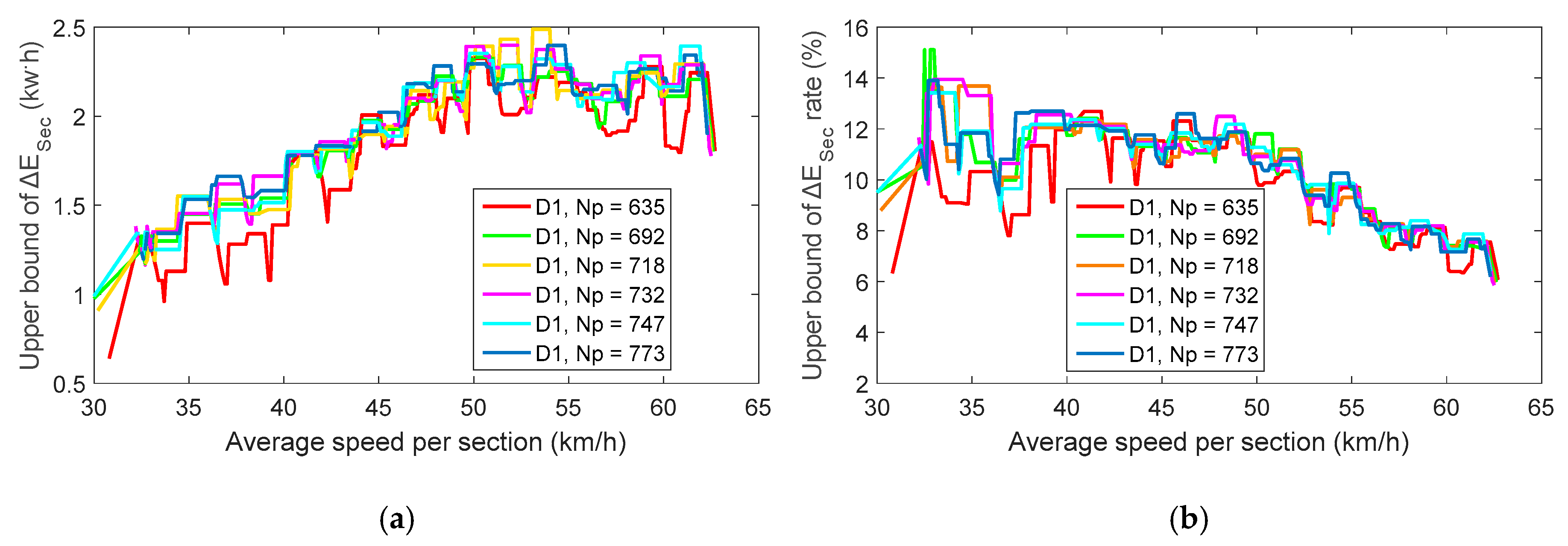
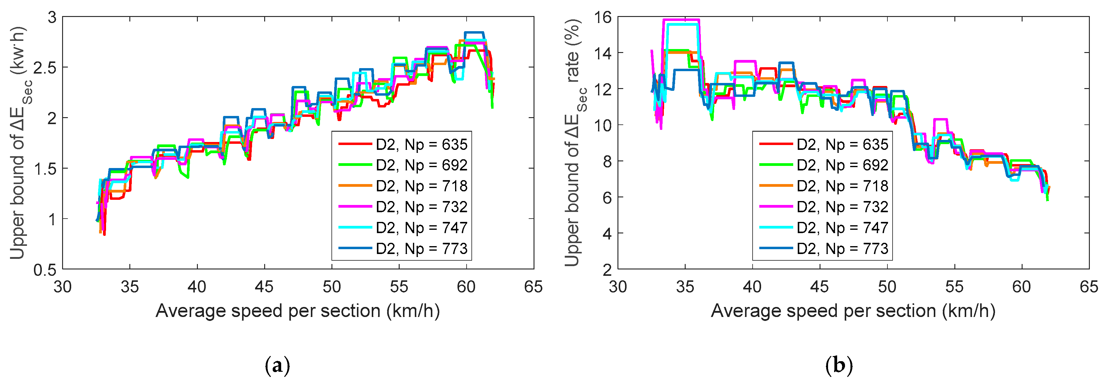
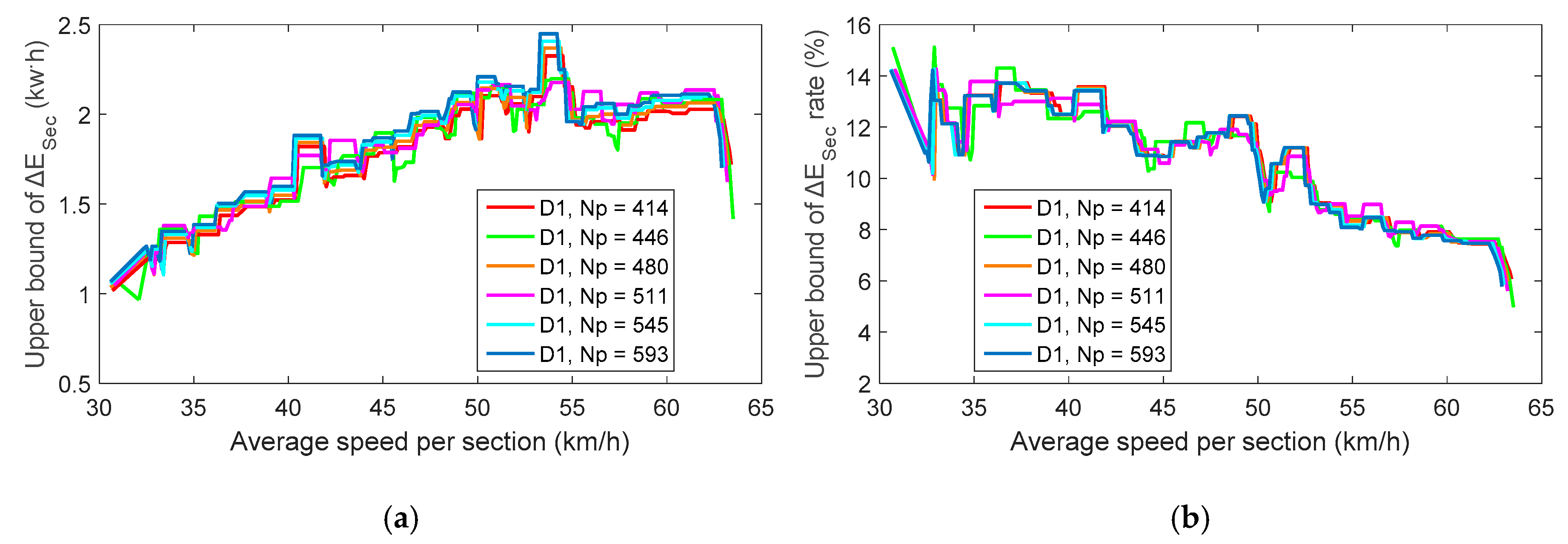
To deep analyze the effects from specific passenger volume conditions on the derived profile boundaries, the weekday and weekend timetable-derived upper bounds, which describe extreme capability space of the given timetables using the optimized driving control solution, are summarized and compared (see
Figure 18,
Figure 19,
Figure 20 and
Figure 21) to demonstrate the energy conservation characteristics with multiple factors.
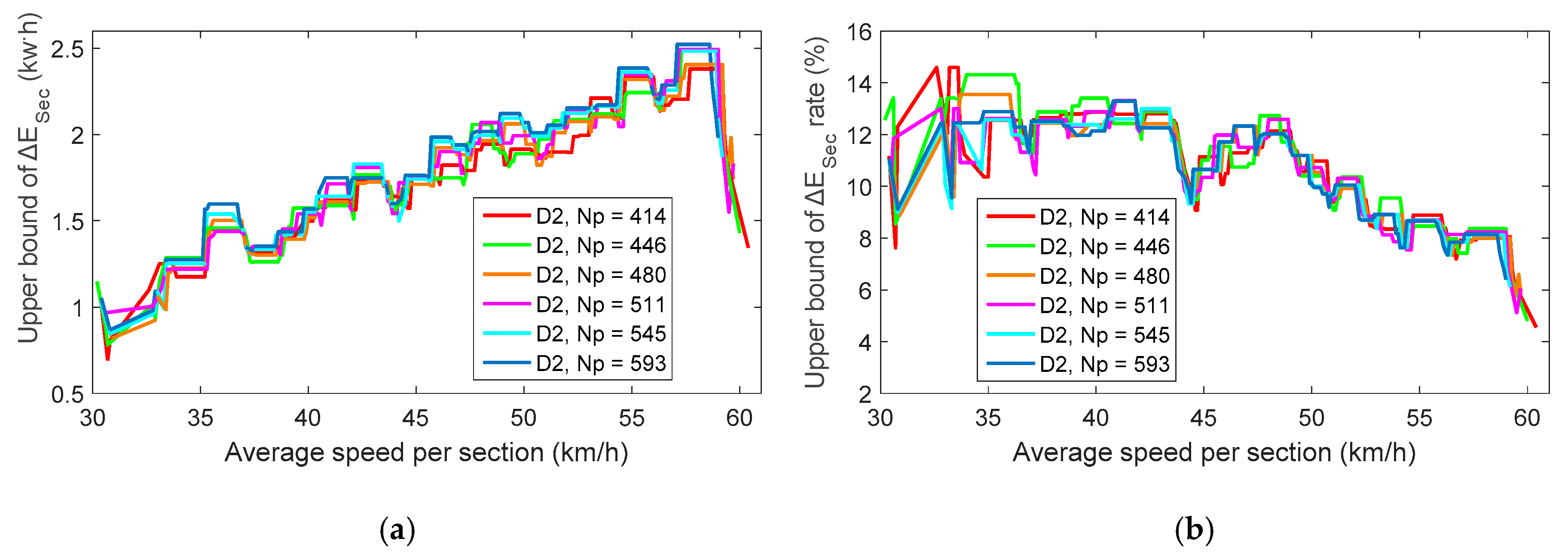
Figure 18 and
Figure 19 depict the passenger volume-based upper bounds covering the energy conservation profiles for both the SH-TQ and TQ-SH weekday timetable, in which the different colors of the boundary curves represent the adopted passenger volume samples in the energy conservation capability evaluation. Similarly,
Figure 20 and
Figure 21 show the computed upper bounds from the weekend timetable in both directions. From the figures, it is easy to find out the similarly consistent trend toward both the energy reduction and energy saving rate when varied passenger load rates are assumed. An increasing upper bound can be derived as a larger average interstation speed no matter whether the passenger load is high or low. At the same time, the upper bounds fall gradually with the increased average running speed per section. However, it is difficult to find out the differences due to the passenger load condition directly from the neighboring upper bound curves. To realize numerical comparisons, the linear curve fitting method is applied to obtain the analytic forms of the boundaries, and thus the fitting slopes of the boundaries are computed and summarized. The fitting slope of an upper bound curve indicates the slope value of a fitted straight line that represents the approximated linear model of the boundary profile.
Table 5 and
Table 6 summarize the comparison results of fitting slopes of the ASS-REN-PLF and ASS-RER-PLF upper boundaries.
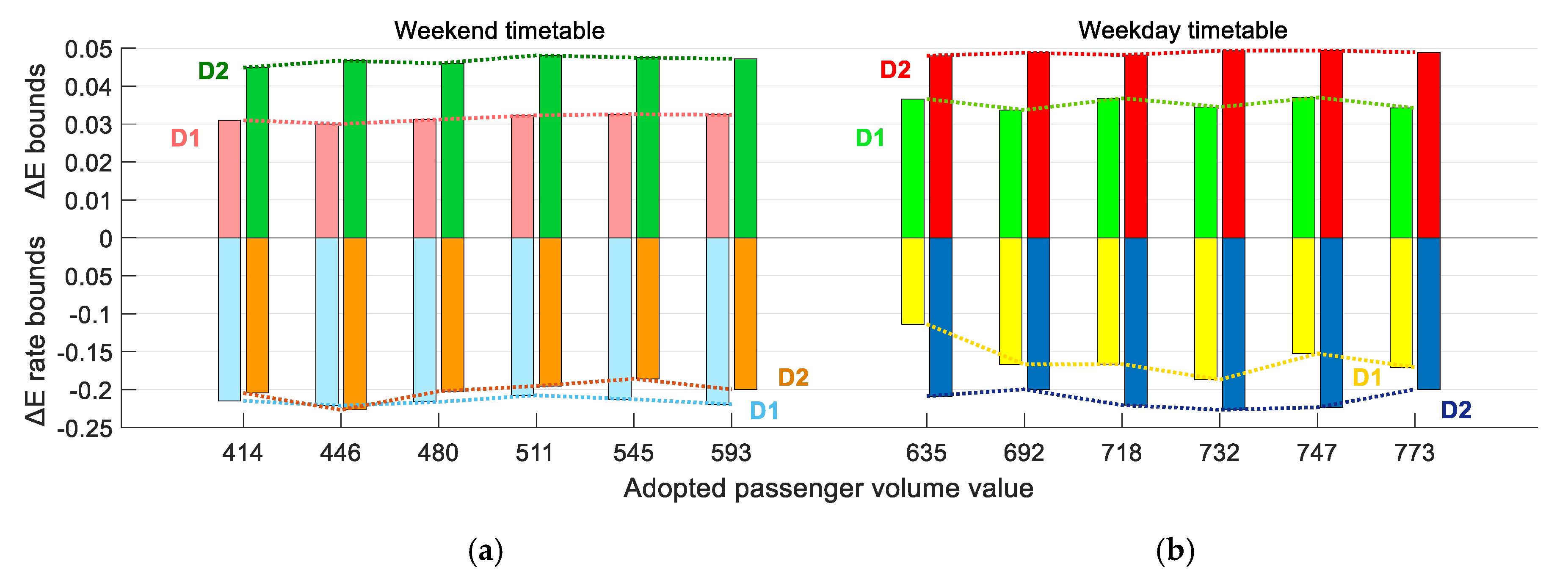
From the results in the tables, similar fitting results can be found in the same direction with these two involved timetable schemes, except for the results of the ASS-RER-PLF profile in the SH-TQ direction. Differences still exist due to the adopted passenger volume value, which indicate that the passenger load condition should be taken into consideration in fully exploring the potential of energy conservation for a time schedule scheme. To show the details of the comparison results, the derived fitting slopes of both the ASS-REN-PLF and ASS-RER-PLF profile boundaries are given in
Figure 22, where the symbol ‘D1’ and ‘D2’ represent the SH-TQ and TQ-SH directions respectively.
It is clear that the fitting slopes vary with the operation direction except for upper bounds of the energy saving rate-related fitting results based on the weekend timetable. The slopes of the weekday timetable-based ASS-REN-PLF upper bounds in D2 and the weekend timetable-based ASS-REN-PLF upper bound-based fitting results in both D1 and D2 do not change greatly with a varied passenger volume. Under the weekday D1 case with respect to the ASS-REN-PLF upper bounds, the volume Np = 747 realizes a maximum fitting slope, which indicates a shaper increase of the upper bound to saved tractive energy consumption with a raising average section speed over other Np-derived results. The situation for the ASS-RER-PLF boundary fitting is much different. The volume Np = 446 for a weekend achieves the maximum fitting slope in both the D1 and D2 directions against other Np conditions. For the weekday timetable-based comparison, a maximum fitting slope is activated by the same condition Np = 732 in both the two directions. According to the changing trend with the passenger load condition, we can draw the conclusion that the identified boundaries with respect to both the ASS-REN-PLF and ASS-RER-PLF profiles vary with different passenger load conditions, while the changing rates of the derived boundaries, including the growing rate for ASS-REN-PLF and decrease rate for ASS-RER-PLF, do not change monotonously. Therefore, to better utilize capability of the proposed BFO-based energy efficient train driving control method, the timetable scheme is suggested to be established or updated by matching the identified ASS-REN-PLF and ASS-RER-PLF profile boundaries, which is significant to accomplish the energy conservation purpose from the operation organization perspective.
5. Conclusions and Future Work
The main contribution of this paper is to give a case study for boundary identification of the energy conservation capability by using the optimized train driving control method. An energy- efficient driving control solution using the Bacterial Foraging Optimization algorithm. Based on that, the connection between the energy saving space of the timetable and the specific influencing factor is described with the derived energy conservation train speed profiles. The proposed energy efficient optimization method and the boundary identification solution are implemented with the data of the Beijing Metro Batong Line. Results of the case study show that the developed approach can realize the quantitative evaluation of achievable space and boundaries for the energy saving capability with a given timetable. A maximum average energy saving rate of 8.20% per section can be realized with the involved timetables by using the BFO-based solution, and an extreme reduction rate of 15.07% is achieved for the weekend timetable. A series of tractive energy saving capability boundaries have been obtained in the case study, which reveal the relationship with the average speed per section and the passenger load condition. The results could give important implications to transit operators, management departments and engineers that the energy conservation operations should be tightly connected with the practical situation and dynamic requirement of the rail transit system.
It should be noticed that this research only concerns the train’s tractive energy consumption in the capability evaluation and boundary identification. In our future work, the regenerative braking factor will be involved in the evaluation of energy conservation profile boundaries with the energy efficient control solution comprehensively under the given timetable schemes. Several influencing factors, including the adopted regenerative braking strategy, capability of the energy storage system and the cooperation of the trains’ movement, will be jointly analyzed with the timetable parameters. Additionally, the effects from the advanced system design, e.g., the lightweight trains with the novel materials, the energy efficient metro infrastructures, and the effective energy storage equipment, are also planned to be investigated to carry out more general analyses on the energy conservation topic. According to the practical operation of the urban rail transit system, this study will be performed continuously for Batong Line and more other metro lines based on the field experiences.


