Finite-Element Simulation for Thermal Modeling of a Cell in an Adiabatic Calorimeter

 ,
,  , ,
, ,  and
and 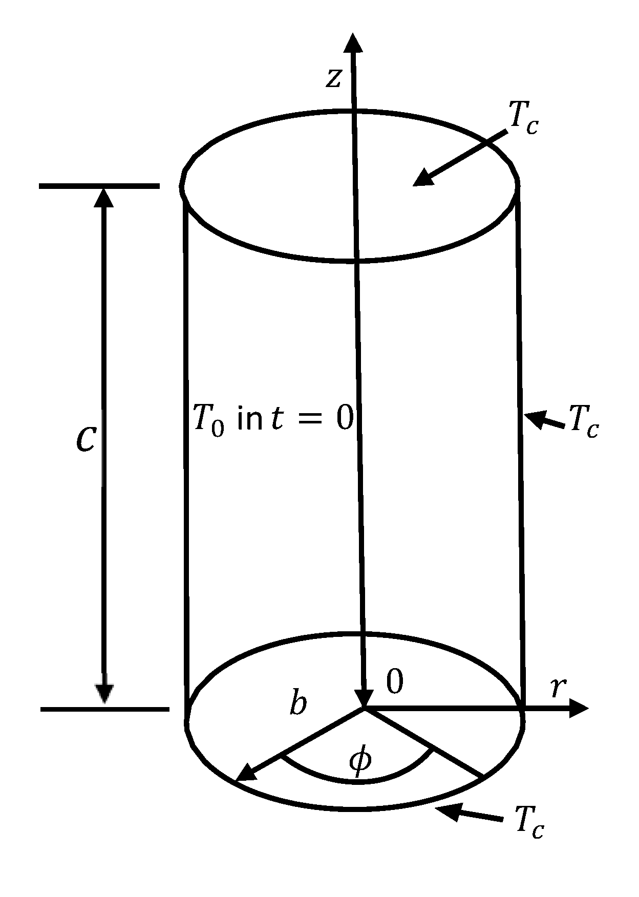
Abstract
:1. Introduction
2. Theoretical Analysis
Mathematical Formulation
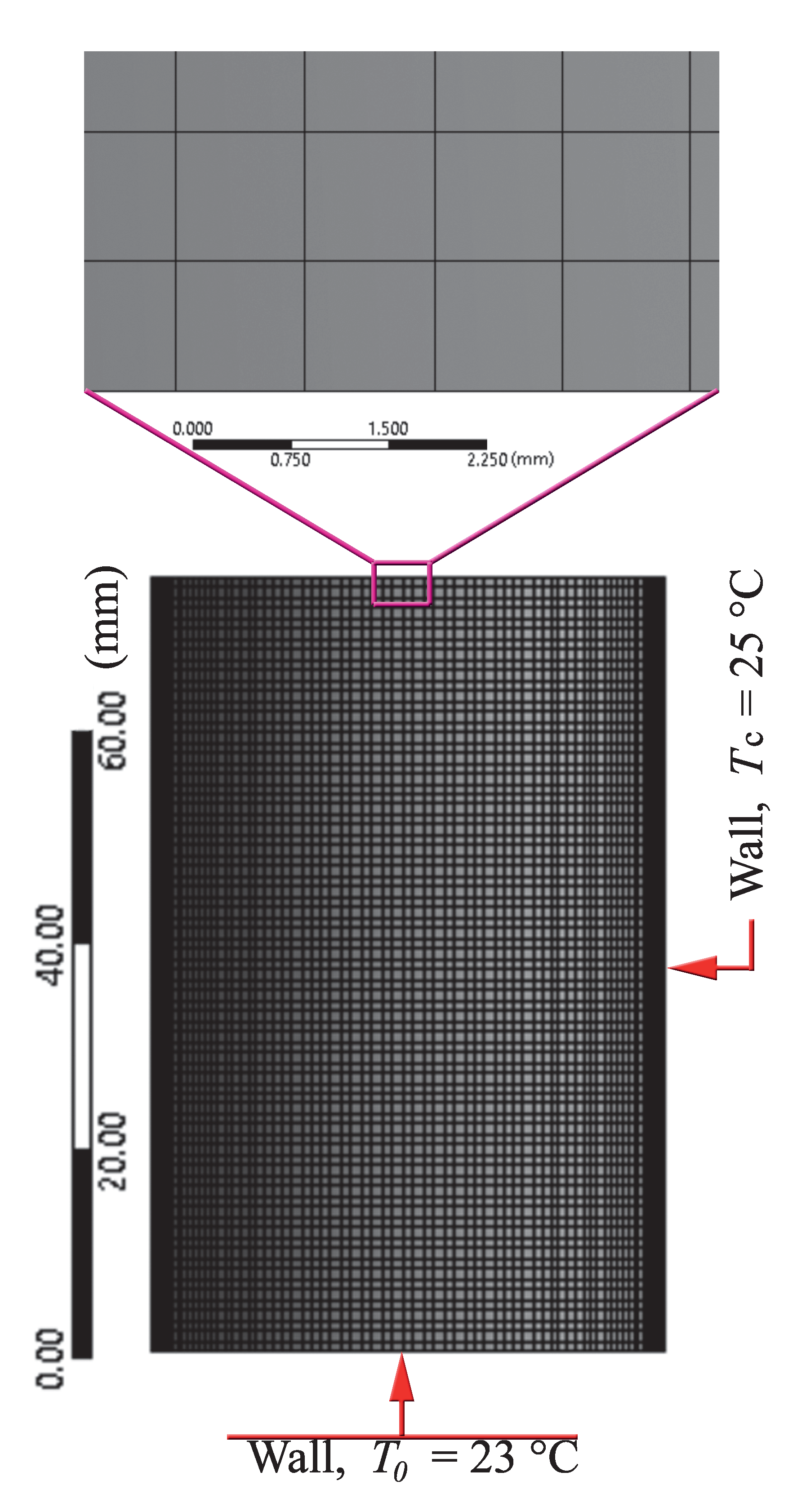
3. Numerical Solution
Model to Compare the Analytical Solution
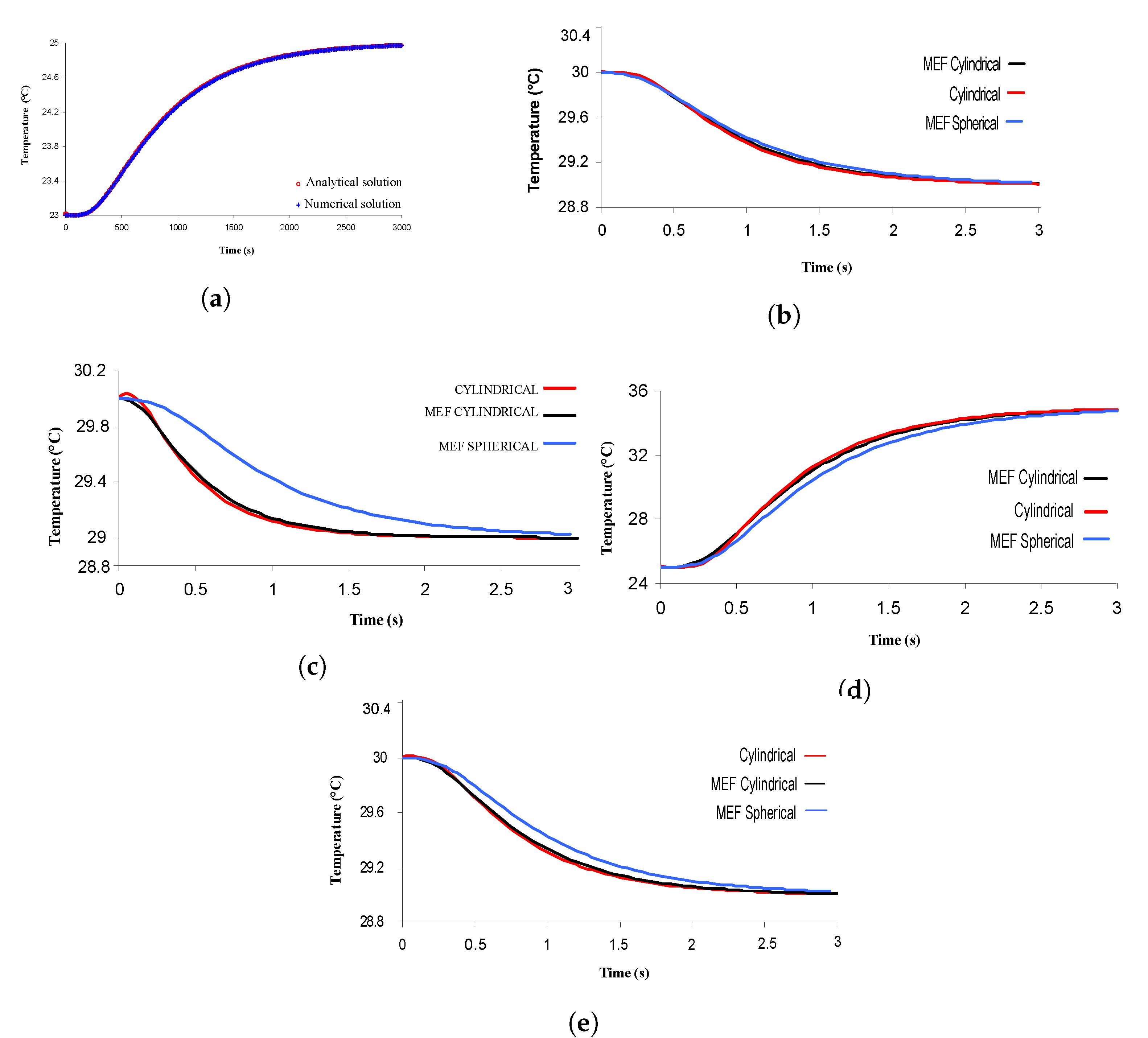
4. Analysis Results
5. Discussion
6. Conclusions
Author Contributions
Funding
Conflicts of Interest
Abbreviations
| Q | Amount of heat |
| m | Mass |
| Temperature variation | |
| I | Current |
| V | Voltage |
| t | Time |
| °C | Celsius grade |
| Thermal diffusivity | |
| k | Thermal conductivity |
| Density | |
| Heat capacity | |
| b | Constant in radial coordinates |
| c | Constant in z coordinates |
| Temperature constant | |
| Represent a change of variable for T | |
| Initially temperature | |
| Bessel functions of order | |
| Eigenfunction | |
| Bessel functions of order | |
| Solution for Bessel functions of order | |
| Eigenvalue evaluated in radius b | |
| Summation of eigenvalue evaluated in radius b | |
| Eigenfunction for z coordinate | |
| Summation of eigenvalue evaluated in height | |
| C | Normal function |
| Bessel functions evaluated in 0 | |
| CENAM | Centro Nacional de Metrologia |
References
- Hoseinzadeh, S.; Heyns, P.S.; Kariman, H. Numerical investigation of heat transfer of laminar and turbulent pulsating Al2O3/water nanofluid flow. Int. J. Numer. Methods Heat Fluid Flow 2019, 30, 1149–1166. [Google Scholar] [CrossRef]
- Sarafraz, M.; Safaei, M.R. Diurnal thermal evaluation of an evacuated tube solar collector (ETSC) charged with graphene nanoplatelets-methanol nano-suspension. Renew. Energy 2019, 142, 364–372. [Google Scholar] [CrossRef]
- Tan, Z.C.; Shi, Q.; Liu, B.P.; Zhang, H.T. A fully automated adiabatic calorimeter for heat capacity measurement between 80 and 400 K. J. Therm. Anal. Calorim. 2008, 92, 367–374. [Google Scholar] [CrossRef]
- Lang, B.E.; Boerio-Goates, J.; Woodfield, B.F. Design and construction of an adiabatic calorimeter for samples of less than 1 cm3 in the temperature range T = 15 K to T = 350 K. J. Chem. Thermodyn. 2006, 38, 1655–1663. [Google Scholar] [CrossRef]
- Kobashi, K.; Kyômen, T.; Oguni, M. Construction of an adiabatic calorimeter in the temperature range between 13 and 505 K, and thermodynamic study of 1-chloroadamantane. J. Phys. Chem. Solids 1998, 59, 667–677. [Google Scholar] [CrossRef]
- Sorai, M.; Kaji, K.; Kaneko, Y. An automated adiabatic calorimeter for the temperature range 13 K to 530 K The heat capacities of benzoic acid from 15 K to 305 K and of synthetic sapphire from 60 K to 505 K. J. Chem. Thermodyn. 1992, 24, 167–180. [Google Scholar] [CrossRef]
- Tan, Z.C.; Shi, Q.; Liu, X. Construction of High-Precision Adiabatic Calorimeter and Thermodynamic Study on Functional Materials. In Calorimetry: Design, Theory and Applications in Porous Solids; IntechOpen: Rijeka, Croatia, 2018; p. 1. [Google Scholar] [CrossRef] [Green Version]
- Matsuo, T.; Suga, H. Adiabatic microcalorimeters for heat capacity measurement at low temperature. Thermochim. Acta 1985, 88, 149–158. [Google Scholar] [CrossRef]
- Magee, J.W.; Deal, R.J.; Blanco, J.C. High-temperature adiabatic calorimeter for constant-volume heat capacity measurements of compressed gases and liquids. J. Res. Natl. Inst. Stand. Technol. 1998, 103, 63. [Google Scholar] [CrossRef]
- Sun, M.T.; Chang, C.H. The error analysis of a steady-state thermal conductivity measurement method with single constant temperature region. J. Heat Transf. 2007. [Google Scholar] [CrossRef]
- Yari, A.; Hosseinzadeh, S.; Galogahi, M. Two-dimensional numerical simulation of the combined heat transfer in channel flow. Int. J. Recent Adv. Mech. Eng. 2014, 3, 55–67. [Google Scholar] [CrossRef]
- Kaur, G.; Singh, M.; Kumar, J.; De Beer, T.; Nopens, I. Mathematical Modelling and Simulation of a Spray Fluidized Bed Granulator. Processes 2018, 6, 195. [Google Scholar] [CrossRef] [Green Version]
- Al-Najem, N.; Özişik, M. On the solution of three-dimensional inverse heat conduction in finite media. Int. J. Heat Mass Transf. 1985, 28, 2121–2128. [Google Scholar] [CrossRef]
- Renaud, J.; Rossomme, S.; Sarfehnia, A.; Vynckier, S.; Palmans, H.; Kacperek, A.; Seuntjens, J. Development and application of a water calorimeter for the absolute dosimetry of short-range particle beams. Phys. Med. Biol. 2016, 61, 6602–6619. [Google Scholar] [CrossRef] [PubMed] [Green Version]
- Amoabeng, K.O.; Lee, K.H.; Choi, J.M. Modeling and Simulation Performance Evaluation of a Proposed Calorimeter for Testing a Heat Pump System. Energies 2019, 12, 4589. [Google Scholar] [CrossRef] [Green Version]
- Karvinen, H.; Hasani Aleni, A.; Salminen, P.; Minav, T.; Vilaça, P. Thermal Efficiency and Material Properties of Friction Stir Channelling Applied to Aluminium Alloy AA5083. Energies 2019, 12, 1549. [Google Scholar] [CrossRef] [Green Version]
- Mohammed, H.A.; Narrein, K. Thermal and hydraulic characteristics of nanofluid flow in a helically coiled tube heat exchanger. Int. Commun. Heat Mass Transf. 2012. [Google Scholar] [CrossRef]
- Pitarch, J.L.; Sala, A.; de Prada, C. A Systematic Grey-Box Modeling Methodology via Data Reconciliation and SOS Constrained Regression. Processes 2019, 7, 170. [Google Scholar] [CrossRef] [Green Version]
- Moreno-Piraján, J.C.; Giraldo, L. Isoperibolic Titration Calorimetry as a Tool for the Prediction of Thermodynamic Properties of Cyclodextrins. Energies 2008, 1, 93–104. [Google Scholar] [CrossRef]
- Özisik, N.; Bayazitoglu, Y.A. Elements of Heat Transfer; McGraw-Hill: New York, NY, USA, 1988. [Google Scholar]
- Zhi-Cheng, T.; Jinchun, Y.; Yi, S.; Shuxia, C.; Lixing, Z. An adiabatic calorimeter for heat capacity measurements in the temperature range 300–600 K and pressure range 0.1–15 MPa. Thermochim. Acta 1991, 183, 29–38. [Google Scholar] [CrossRef]
- Zhong, Q.; Dong, X.; Zhao, Y.; Wang, J.; Zhang, H.; Li, H.; Guo, H.; Shen, J.; Gong, M. Adiabatic calorimeter for isochoric specific heat capacity measurements and experimental data of compressed liquid R1234yf. J. Chem. Thermodyn. 2018, 125, 86–92. [Google Scholar] [CrossRef]
- Gadalla, M.; Ghommem, M.; Bourantas, G.; Miller, K. Modeling and Thermal Analysis of a Moving Spacecraft Subject to Solar Radiation Effect. Processes 2019, 7, 807. [Google Scholar] [CrossRef] [Green Version]
- Zhu, H.; Sun, B.; Jiang, J.; Xu, W. Measurement of hazardous reactions under extreme conditions with a house-built high-performance adiabatic calorimeter. J. Therm. Anal. Calorim. 2020. [Google Scholar] [CrossRef]
- Kossoy, A. An in-depth analysis of some methodical aspects of applying pseudo-adiabatic calorimetry. Thermochim. Acta 2020, 683. [Google Scholar] [CrossRef]
- Choi, Y.; Jeon, K.; Park, Y.; Hyun, S. Numerical simulation of heat-loss compensated calorimeter. Int. J. Comput. Methods Exp. Meas. 2019, 7, 285–296. [Google Scholar] [CrossRef]
- Ding, J.; Yu, L.; Wang, J.; Xu, Q.; Yang, S.; Ye, S. A symmetric dual-channel accelerating rate calorimeter with the varying thermal inertia consideration. Thermochim. Acta 2019, 678. [Google Scholar] [CrossRef]
- Ivsic, B.; Dadic, M.; Malaric, R.; Martinovic, Z. Thermal considerations on adiabatic coaxial line for microcalorimeter measurements. In Proceedings of the 2019 2nd International Colloquium on Smart Grid Metrology (SMAGRIMET), Split, Croatia, 9–12 April 2019. [Google Scholar] [CrossRef]
- Sarafraz, M.; Arya, A.; Nikkhah, V.; Hormozi, F. Thermal performance and viscosity of biologically produced silver/coconut oil nanofluids. Chem. Biochem. Eng. Q. 2016, 30, 489–500. [Google Scholar] [CrossRef]
- Sarafraz, M.M.; Tlili, I.; Tian, Z.; Bakouri, M.; Safaei, M.R.; Goodarzi, M. Thermal Evaluation of Graphene Nanoplatelets Nanofluid in a Fast-Responding HP with the Potential Use in Solar Systems in Smart Cities. Appl. Sci. 2019, 9, 2101. [Google Scholar] [CrossRef] [Green Version]


© 2020 by the authors. Licensee MDPI, Basel, Switzerland. This article is an open access article distributed under the terms and conditions of the Creative Commons Attribution (CC BY) license (http://creativecommons.org/licenses/by/4.0/).
Share and Cite
González-Durán, J.E.E.; Rodríguez-Reséndiz, J.; Ramirez, J.M.O.; Zamora-Antuñano, M.A.; Lira-Cortes, L. Finite-Element Simulation for Thermal Modeling of a Cell in an Adiabatic Calorimeter. Energies 2020, 13, 2300. https://0-doi-org.brum.beds.ac.uk/10.3390/en13092300
González-Durán JEE, Rodríguez-Reséndiz J, Ramirez JMO, Zamora-Antuñano MA, Lira-Cortes L. Finite-Element Simulation for Thermal Modeling of a Cell in an Adiabatic Calorimeter. Energies. 2020; 13(9):2300. https://0-doi-org.brum.beds.ac.uk/10.3390/en13092300
Chicago/Turabian StyleGonzález-Durán, José Eli Eduardo, Juvenal Rodríguez-Reséndiz, Juan Manuel Olivares Ramirez, Marco Antonio Zamora-Antuñano, and Leonel Lira-Cortes. 2020. "Finite-Element Simulation for Thermal Modeling of a Cell in an Adiabatic Calorimeter" Energies 13, no. 9: 2300. https://0-doi-org.brum.beds.ac.uk/10.3390/en13092300