Wind Turbine Systematic Yaw Error: Operation Data Analysis Techniques for Detecting It and Assessing Its Performance Impact


 ,
,
Abstract
:
1. Introduction
- contributing to the SCADA-based methodologies for diagnosing systematic yaw error;
- assessing the impact of systematic yaw error through innovative techniques based on SCADA data analysis.
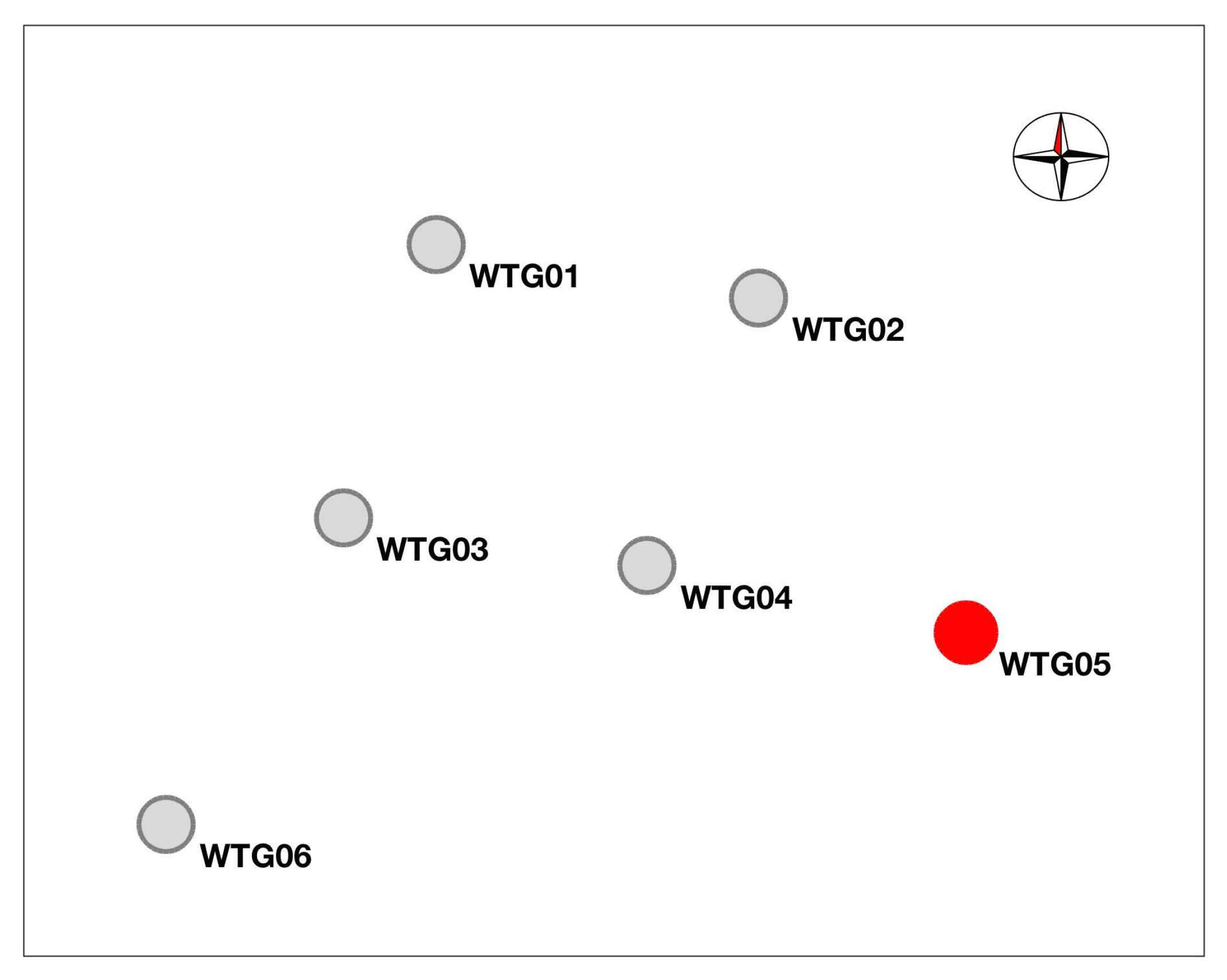
2. The Test Case and the Data Set
- goes from 1st January 2017 to 1st January 2018: it is a data set prior to the yaw error correction on WTG05;
- goes from 1st January 2020 to 1st April 2020: it is a data set posterior to the yaw error correction on WTG05.
- nacelle wind speed v;
- nacelle wind direction ;
- nacelle position ;
- power production P;
- rotor speed ;
- generator speed ;
- blade pitch angle .
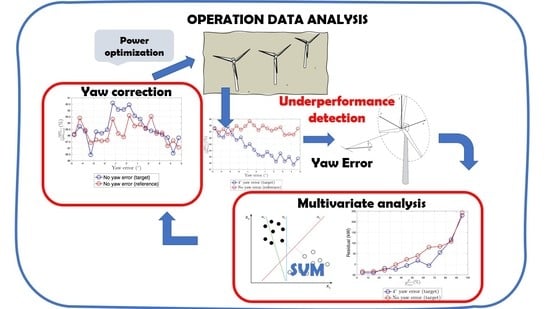
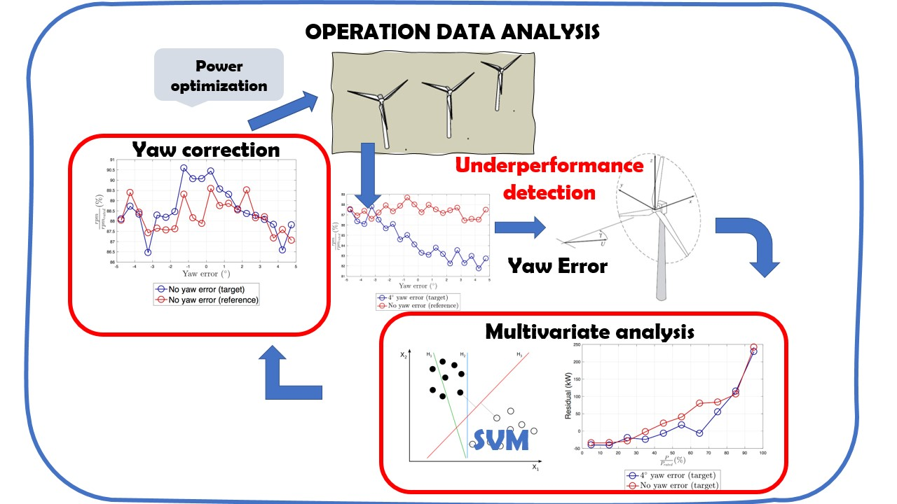
3. Methods
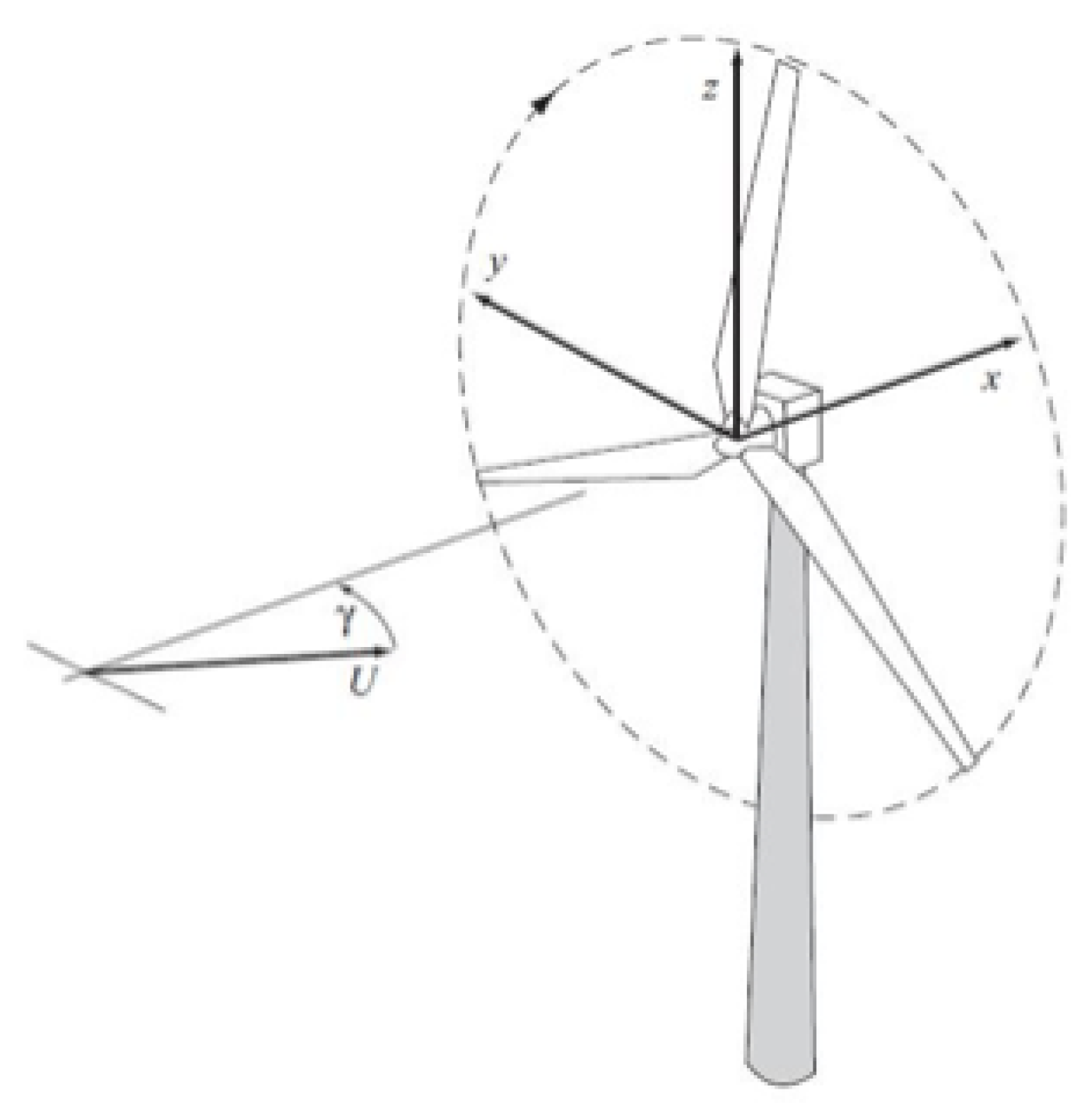
3.1. Yaw Error Detection
- filter the data on wind turbine operation time, using the appropriate time counter;
- filter the data on a narrow wind speed interval in Region II.
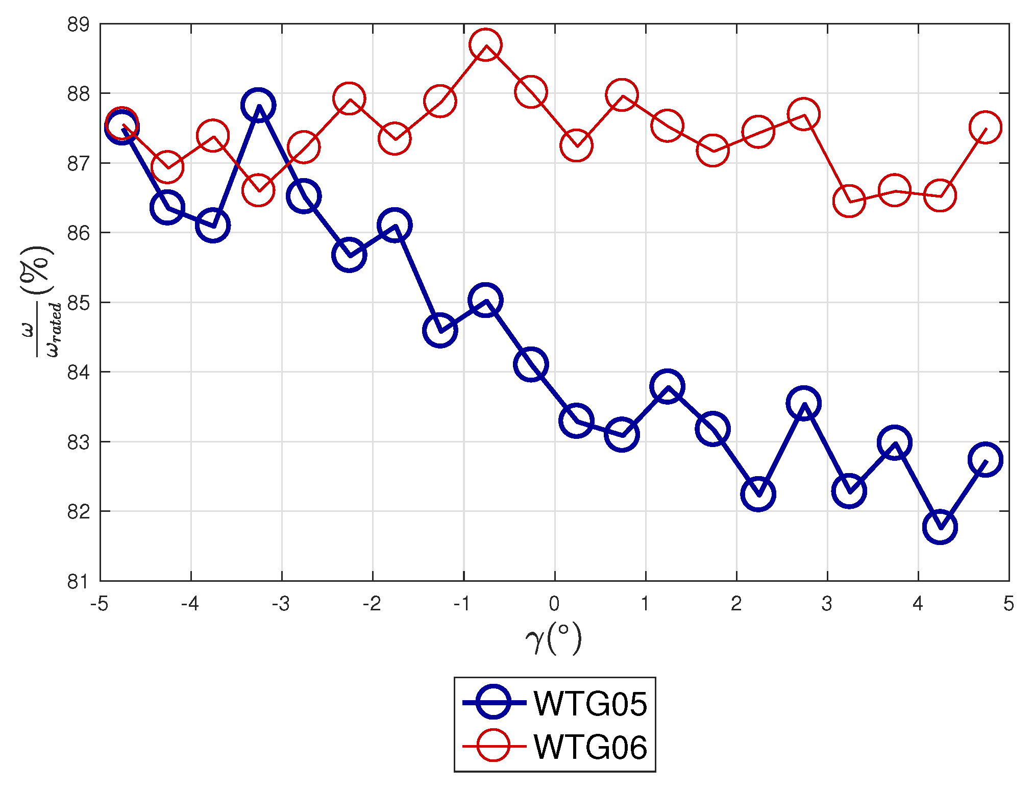
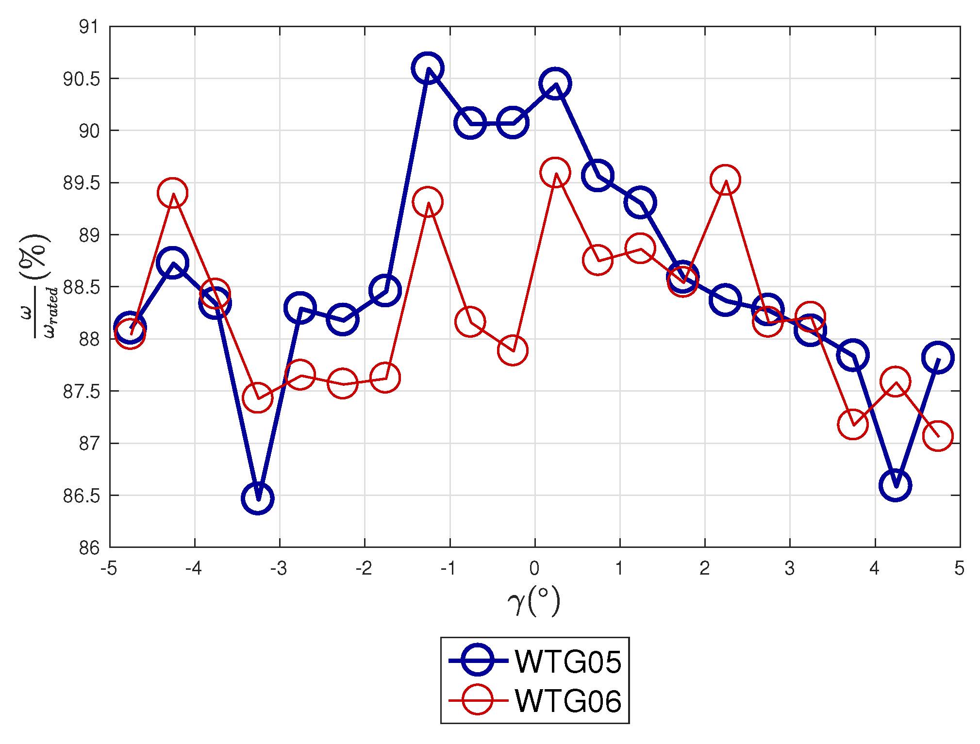
- compute the average yaw error–rotor speed curve. Data can be averaged on yaw error intervals of, for example, or .
- the curve should have its maximum for and diminish for increasing absolute value of . On the other way round, if there is a systematic yaw error, the curve is clearly asymmetric and has its maximum at the value of corresponding to the systematic error.
- if all the wind turbines in the farm are well aligned, the observed average should have the same order of magnitude for all the wind turbines. If a wind turbine is losing rotor speed, it is under-performing.
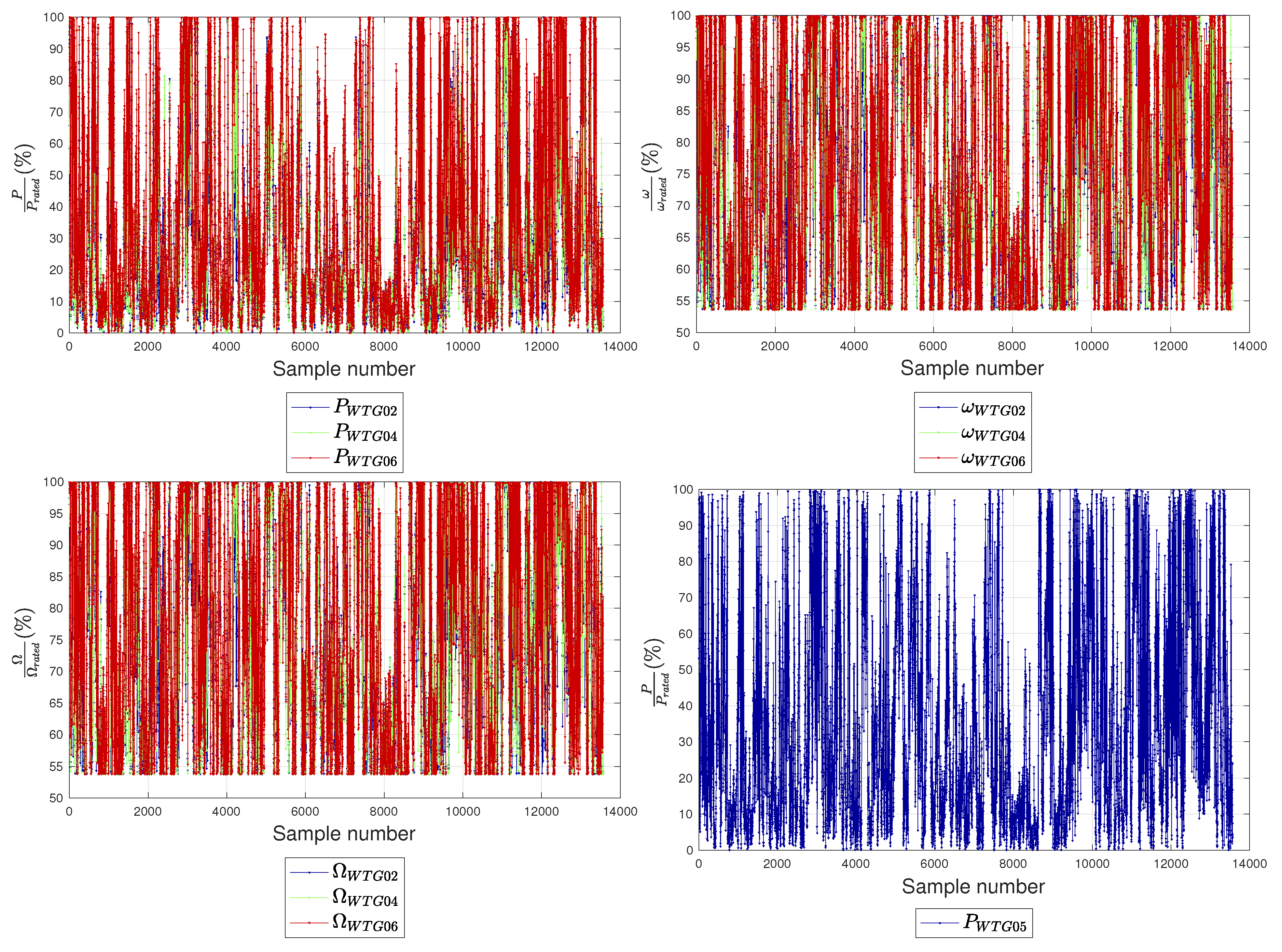
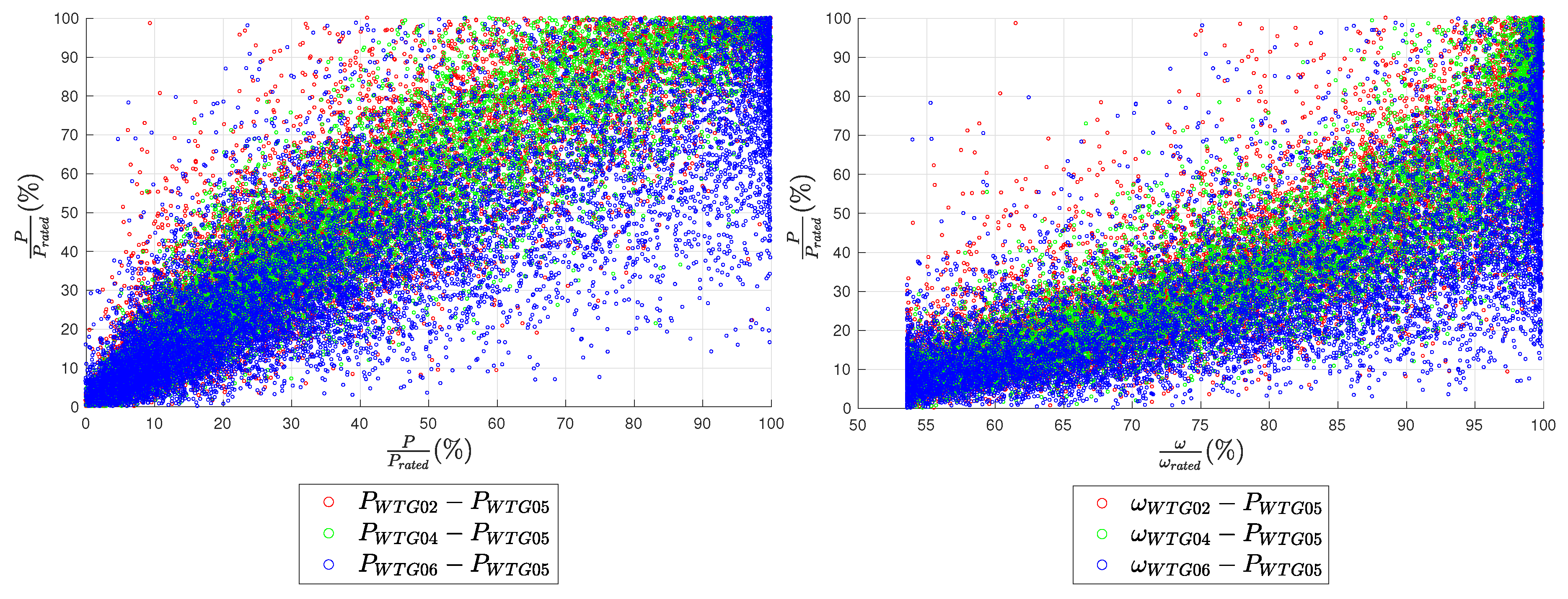
3.2. Support Vector Regression and Data Set Analysis
- power of WTG02: ;
- power of WTG04: ;
- power of WTG06: ;
- rotor speed of WTG02: ;
- rotor speed of WTG04: ;
- rotor speed of WTG06: ;
- generator speed of WTG02: ;
- generator speed of WTG04: ;
- generator speed of WTG06: .
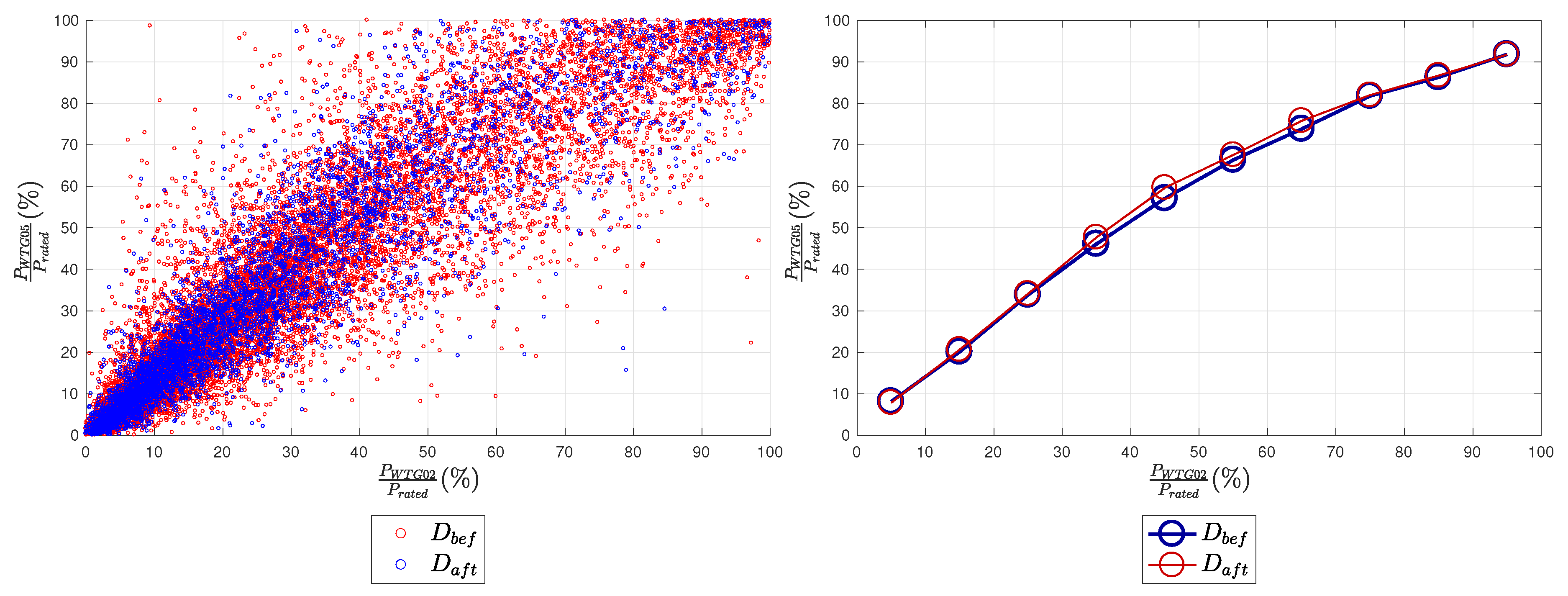
- train the model on a pre-correction data set;
- predict new values on a pre-correction data set;
- predict new values on a post-correction data set.
3.3. Performance Analysis
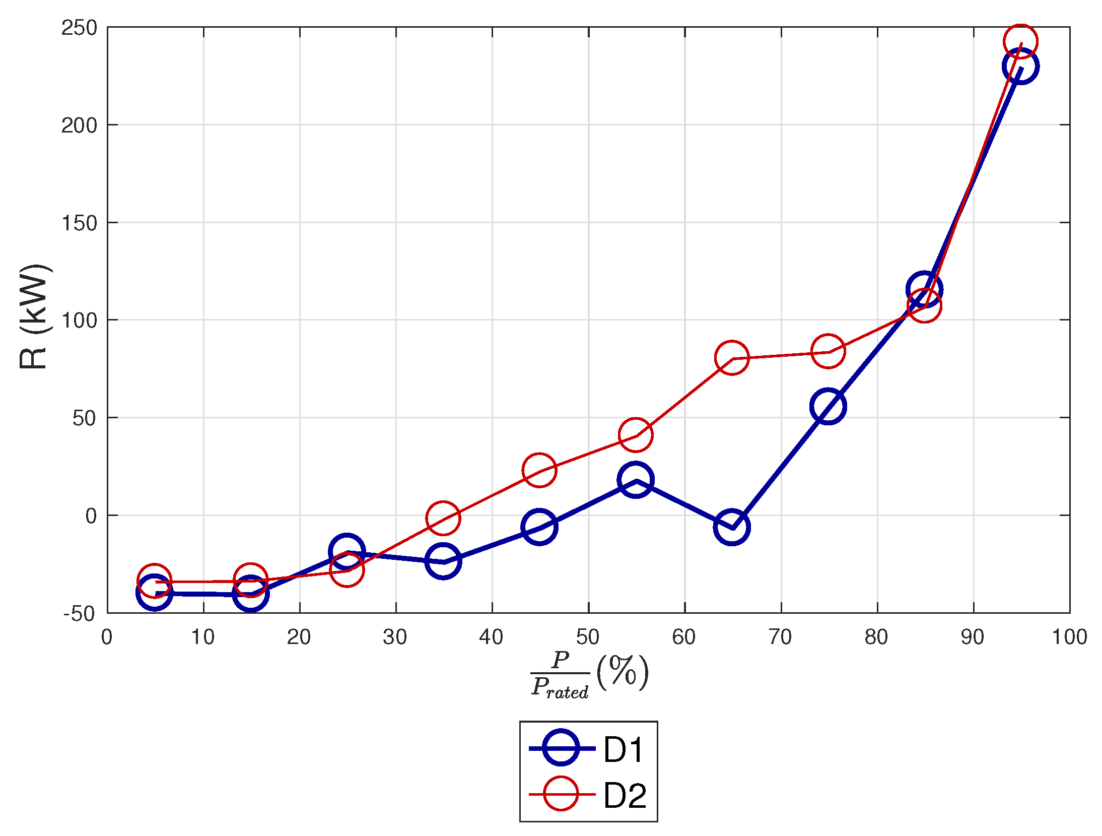
- is randomly divided into two subsets: D0 (a random selection of of the data set) and D1 (the remainder of the data set). D0 is used for training the regression, D1 is used for testing the regression. The convergence of model training is verified through the MATLAB® fitrsvm routine.
- (also named D2 for notation consistency) is used to quantify the performance deviation with respect to D1 (and therefore ).
4. Results
4.1. Yaw Error Diagnosis
4.2. Performance Assessment
5. Conclusions
- Despite the fact that SCADA data do not provide upwind flow measurements, it is nevertheless possible (and recommended) to employ them for reliably diagnosing systematic yaw errors. The main innovation of this study has been targeting the rotor speed, because in Region II it directly depends on the torque exerted on the rotor and torque is lost if the yaw angle is systematically non-zero when it should be zero. Analyzing the properties of the yaw error–rotor speed curve, for each single wind turbine and comparing wind turbines in a wind farm, it is possible to obtain meaningful indications about the presence of systematic yaw errors.
- As discussed in [7], the effect of yaw error should be read in light of the wind turbine control. The energy yield is affected by the systematic yaw error in particular in Region II, when the torque and the rotor speed increase with the wind and the blade pitch angle is practically set to 0. Near the cut-in and near rated power, the importance of pitch control increases and the yaw error is less important. The net effect of this on wind turbine operation can be estimated from the test case considered in this work: a systematic yaw error of can affect the AEP of the wind turbine for the order of 1.5%.
Author Contributions
Acknowledgments
Conflicts of Interest
Nomenclature
| List of the mathematical symbols. | |
| Symbol | Meaning |
| v | Nacelle wind speed |
| Nacelle wind direction | |
| Nacelle position | |
| P | Power production |
| Rotor speed | |
| Generator speed | |
| Blade pitch angle | |
| Yaw error | |
| Asymmetry Index | |
| Discrepancy Index | |
| r | Pearson coefficient |
| R | Residuals between measurement and model estimate |
| Average percentage residual | |
| E | Energy Yield |
| List of the abbreviations. | |
| Acronym | Meaning |
| AEP | Annual Energy Production |
| GP | Gaussian Process |
| HAWT | Horizontal-Axis Wind Turbine |
| IEC | International Electrotechnical Commission |
| LASSO | Least Absolute Shrinkage and Selection Operator |
| PCR | Principal Component Regression |
| SCADA | Supervisory Control And Data Acquisition |
| SVM | Support Vector Machine |
| SVR | Support Vector Regression |
| WTG | Wind Turbine Generator |
References
- McKenna, R.; vd Leye, P.O.; Fichtner, W. Key challenges and prospects for large wind turbines. Renew. Sustain. Energy Rev. 2016, 53, 1212–1221. [Google Scholar] [CrossRef]
- Saenz-Aguirre, A.; Fernandez-Gamiz, U.; Zulueta, E.; Aramendia, I.; Teso-Fz-Betono, D. Flow control based 5 MW wind turbine enhanced energy production for hydrogen generation cost reduction. Int. J. Hydrog. Energy 2020. [Google Scholar] [CrossRef]
- Burton, T.; Jenkins, N.; Sharpe, D.; Bossanyi, E. Wind Energy Handbook; John Wiley & Sons: Hoboken, NJ, USA, 2011. [Google Scholar]
- Wan, S.; Cheng, L.; Sheng, X. Effects of yaw error on wind turbine running characteristics based on the equivalent wind speed model. Energies 2015, 8, 6286–6301. [Google Scholar] [CrossRef]
- Schulz, C.; Letzgus, P.; Lutz, T.; Krämer, E. CFD study on the impact of yawed inflow on loads, power and near wake of a generic wind turbine. Wind Energy 2017, 20, 253–268. [Google Scholar] [CrossRef]
- Jeong, M.S.; Kim, S.W.; Lee, I.; Yoo, S.J.; Park, K. The impact of yaw error on aeroelastic characteristics of a horizontal axis wind turbine blade. Renew. Energy 2013, 60, 256–268. [Google Scholar] [CrossRef]
- Dai, J.; Yang, X.; Hu, W.; Wen, L.; Tan, Y. Effect investigation of yaw on wind turbine performance based on SCADA data. Energy 2018, 149, 684–696. [Google Scholar] [CrossRef]
- Cortina, G.; Sharma, V.; Calaf, M. Investigation of the incoming wind vector for improved wind turbine yaw-adjustment under different atmospheric and wind farm conditions. Renew. Energy 2017, 101, 376–386. [Google Scholar] [CrossRef] [Green Version]
- Kragh, K.A.; Hansen, M.H. Potential of power gain with improved yaw alignment. Wind Energy 2015, 18, 979–989. [Google Scholar] [CrossRef]
- Song, D.; Fan, X.; Yang, J.; Liu, A.; Chen, S.; Joo, Y.H. Power extraction efficiency optimization of horizontal-axis wind turbines through optimizing control parameters of yaw control systems using an intelligent method. Appl. Energy 2018, 224, 267–279. [Google Scholar] [CrossRef]
- Karakasis, N.; Mesemanolis, A.; Nalmpantis, T.; Mademlis, C. Active yaw control in a horizontal axis wind system without requiring wind direction measurement. IET Renew. Power Gener. 2016, 10, 1441–1449. [Google Scholar] [CrossRef]
- Shariatpanah, H.; Fadaeinedjad, R.; Rashidinejad, M. A new model for PMSG-based wind turbine with yaw control. IEEE Trans. Energy Convers. 2013, 28, 929–937. [Google Scholar] [CrossRef]
- Song, D.; Yang, J.; Fan, X.; Liu, Y.; Liu, A.; Chen, G.; Joo, Y.H. Maximum power extraction for wind turbines through a novel yaw control solution using predicted wind directions. Energy Convers. Manag. 2018, 157, 587–599. [Google Scholar] [CrossRef]
- Saenz-Aguirre, A.; Zulueta, E.; Fernandez-Gamiz, U.; Lozano, J.; Lopez-Guede, J.M. Artificial Neural Network Based Reinforcement Learning for Wind Turbine Yaw Control. Energies 2019, 12, 436. [Google Scholar] [CrossRef] [Green Version]
- Saenz-Aguirre, A.; Zulueta, E.; Fernandez-Gamiz, U.; Ulazia, A.; Teso-Fz-Betono, D. Performance enhancement of the artificial neural network–based reinforcement learning for wind turbine yaw control. Wind Energy 2019. [Google Scholar] [CrossRef]
- Astolfi, D.; Castellani, F.; Natili, F. Wind Turbine Yaw Control Optimization and Its Impact on Performance. Machines 2019, 7, 41. [Google Scholar] [CrossRef] [Green Version]
- Campagnolo, F.; Petrović, V.; Bottasso, C.L.; Croce, A. Wind tunnel testing of wake control strategies. In Proceedings of the IEEE American Control Conference (ACC), Boston, MA, USA, 6–8 July 2016; pp. 513–518. [Google Scholar]
- Gebraad, P.; Teeuwisse, F.; Van Wingerden, J.; Fleming, P.A.; Ruben, S.; Marden, J.; Pao, L. Wind plant power optimization through yaw control using a parametric model for wake effects—A CFD simulation study. Wind Energy 2016, 19, 95–114. [Google Scholar] [CrossRef]
- Fleming, P.; Churchfield, M.; Scholbrock, A.; Clifton, A.; Schreck, S.; Johnson, K.; Wright, A.; Gebraad, P.; Annoni, J.; Naughton, B.; et al. Detailed field test of yaw-based wake steering. J. Phys. Conf. Ser. 2016, 753, 052003. [Google Scholar] [CrossRef] [Green Version]
- Dai, J.; Yang, X.; Yang, W.; Gao, G.; Li, M. Further Study on the Effects of Wind Turbine Yaw Operation for Aiding Active Wake Management. Appl. Sci. 2020, 10, 1978. [Google Scholar] [CrossRef] [Green Version]
- Kragh, K.; Hansen, M.; Mikkelsen, T. Improving yaw alignment using spinner based LIDAR. In Proceedings of the 49th AIAA Aerospace Sciences Meeting Including the New Horizons Forum and Aerospace Exposition, Orlando, FL, USA, 4–7 January 2011; p. 264. [Google Scholar]
- Mikkelsen, T.; Angelou, N.; Hansen, K.; Sjöholm, M.; Harris, M.; Slinger, C.; Hadley, P.; Scullion, R.; Ellis, G.; Vives, G. A spinner-integrated wind lidar for enhanced wind turbine control. Wind Energy 2013, 16, 625–643. [Google Scholar] [CrossRef] [Green Version]
- Zhang, L.; Yang, Q. A Method for Yaw Error Alignment of Wind Turbine Based on LiDAR. IEEE Access 2020, 8, 25052–25059. [Google Scholar] [CrossRef]
- Bakhshi, R.; Sandborn, P. Maximizing the returns of LIDAR systems in wind farms for yaw error correction applications. Wind Energy 2020. [Google Scholar] [CrossRef]
- Muljadi, E.; Butterfield, C.P. Pitch-controlled variable-speed wind turbine generation. IEEE Trans. Ind. Appl. 2001, 37, 240–246. [Google Scholar] [CrossRef] [Green Version]
- Ding, Y. Data Science for Wind Energy; CRC Press: Boca Raton, FL, USA, 2019. [Google Scholar]
- Pei, Y.; Qian, Z.; Jing, B.; Kang, D.; Zhang, L. Data-Driven Method for Wind Turbine Yaw Angle Sensor Zero-Point Shifting Fault Detection. Energies 2018, 11, 553. [Google Scholar] [CrossRef] [Green Version]
- Astolfi, D.; Castellani, F.; Terzi, L. An Operation Data-Based Method for the Diagnosis of Zero-Point Shift of Wind Turbines Yaw Angle. J. Sol. Energy Eng. 2020, 142. [Google Scholar] [CrossRef]
- Astolfi, D.; Castellani, F.; Scappaticci, L.; Terzi, L. Diagnosis of wind turbine misalignment through SCADA data. Diagnostyka 2017, 18, 17–24. [Google Scholar]
- Liao, M.; Dong, L.; Jin, L.; Wang, S. Study on rotational speed feedback torque control for wind turbine generator system. In Proceedings of the IEEE International Conference on Energy and Environment Technology, Guilin, China, 16–18 October 2009; Volume 1, pp. 853–856. [Google Scholar]
- Demurtas, G.; Pedersen, T.F.; Zahle, F. Calibration of a spinner anemometer for wind speed measurements. Wind Energy 2016, 19, 2003–2021. [Google Scholar] [CrossRef] [Green Version]
- Astolfi, D.; Castellani, F.; Terzi, L. Wind Turbine Power Curve Upgrades. Energies 2018, 11, 1300. [Google Scholar] [CrossRef] [Green Version]
- Astolfi, D.; Castellani, F.; Fravolini, M.L.; Cascianelli, S.; Terzi, L. Precision Computation of Wind Turbine Power Upgrades: An Aerodynamic and Control Optimization Test Case. J. Energy Resour. Technol. 2019, 141, 051205. [Google Scholar] [CrossRef]
- Astolfi, D.; Castellani, F. Wind turbine power curve upgrades: Part II. Energies 2019, 12, 1503. [Google Scholar] [CrossRef] [Green Version]
- Astolfi, D. A Study of the Impact of Pitch Misalignment on Wind Turbine Performance. Machines 2019, 7, 8. [Google Scholar] [CrossRef] [Green Version]
- IEC. Power Performance Measurements of Electricity Producing Wind Turbines; Technical Report 61400-12; International Electrotechnical Commission: Geneva, Switzerland, 2005. [Google Scholar]
- Van den Berg, G. Wind turbine power and sound in relation to atmospheric stability. Wind Energy 2008, 11, 151–169. [Google Scholar] [CrossRef]
- Wagner, R.; Antoniou, I.; Pedersen, S.M.; Courtney, M.S.; Jørgensen, H.E. The influence of the wind speed profile on wind turbine performance measurements. Wind Energy 2009, 12, 348–362. [Google Scholar] [CrossRef]
- Guo, P.; Infield, D. Wind turbine power curve modeling and monitoring with Gaussian Process and SPRT. IEEE Trans. Sustain. Energy 2018, 11, 107–115. [Google Scholar] [CrossRef] [Green Version]
- Pandit, R.K.; Infield, D. Comparative assessments of binned and support vector regression-based blade pitch curve of a wind turbine for the purpose of condition monitoring. Int. J. Energy Environ. Eng. 2019, 10, 181–188. [Google Scholar] [CrossRef] [Green Version]
- Wagner, R.; Ca nadillas, B.; Clifton, A.; Feeney, S.; Nygaard, N.; Poodt, M.; St Martin, C.; Tüxen, E.; Wagenaar, J. Rotor equivalent wind speed for power curve measurement–comparative exercise for IEA Wind Annex 32. J. Phys. Conf. Ser. 2014, 524, 012108. [Google Scholar] [CrossRef]
- Scheurich, F.; Enevoldsen, P.B.; Paulsen, H.N.; Dickow, K.K.; Fiedel, M.; Loeven, A.; Antoniou, I. Improving the accuracy of wind turbine power curve validation by the rotor equivalent wind speed concept. J. Phys. Conf. Ser. 2016, 753, 072029. [Google Scholar] [CrossRef] [Green Version]
- Smola, A.J.; Schölkopf, B. A tutorial on support vector regression. Stat. Comput. 2004, 14, 199–222. [Google Scholar] [CrossRef] [Green Version]
- Lee, G.; Ding, Y.; Xie, L.; Genton, M.G. A kernel plus method for quantifying wind turbine performance upgrades. Wind Energy 2015, 18, 1207–1219. [Google Scholar] [CrossRef]
- Hwangbo, H.; Ding, Y.; Eisele, O.; Weinzierl, G.; Lang, U.; Pechlivanoglou, G. Quantifying the effect of vortex generator installation on wind power production: An academia-industry case study. Renew. Energy 2017, 113, 1589–1597. [Google Scholar] [CrossRef]
- Refaeilzadeh, P.; Tang, L.; Liu, H. Cross-validation. In Encyclopedia of Database Systems; Springer: Berlin, Germany, 2009; pp. 532–538. [Google Scholar]


| Covariate | Mean (% of Rated) | Coefficient of Variation (%) | Skewness | Kurtosis | |
|---|---|---|---|---|---|
| 29.5 | 85.1 | 1.0 | 3.0 | 0.91 | |
| 30.9 | 84.2 | 0.9 | 2.9 | 0.94 | |
| 38.2 | 83.3 | 0.7 | 2.1 | 0.87 | |
| 75.0 | 21.9 | 0.1 | 1.6 | 0.90 | |
| 75.8 | 22.0 | 0.09 | 1.5 | 0.91 | |
| 78.9 | 22.2 | −0.1 | 1.5 | 0.82 | |
| 75.1 | 21.8 | 0.2 | 1.6 | 0.89 | |
| 75.9 | 21.9 | 0.09 | 1.5 | 0.92 | |
| 78.9 | 22.1 | −0.1 | 1.5 | 0.84 |
| Data Set | ||
|---|---|---|
| 3.3 | 2.9 | |
| 0.3 | −0.3 |
| Data Set | (kW) |
|---|---|
| D1 | −0.9 |
| D2 | 12.5 |
© 2020 by the authors. Licensee MDPI, Basel, Switzerland. This article is an open access article distributed under the terms and conditions of the Creative Commons Attribution (CC BY) license (http://creativecommons.org/licenses/by/4.0/).
Share and Cite
Astolfi, D.; Castellani, F.; Becchetti, M.; Lombardi, A.; Terzi, L. Wind Turbine Systematic Yaw Error: Operation Data Analysis Techniques for Detecting It and Assessing Its Performance Impact. Energies 2020, 13, 2351. https://0-doi-org.brum.beds.ac.uk/10.3390/en13092351
Astolfi D, Castellani F, Becchetti M, Lombardi A, Terzi L. Wind Turbine Systematic Yaw Error: Operation Data Analysis Techniques for Detecting It and Assessing Its Performance Impact. Energies. 2020; 13(9):2351. https://0-doi-org.brum.beds.ac.uk/10.3390/en13092351
Chicago/Turabian StyleAstolfi, Davide, Francesco Castellani, Matteo Becchetti, Andrea Lombardi, and Ludovico Terzi. 2020. "Wind Turbine Systematic Yaw Error: Operation Data Analysis Techniques for Detecting It and Assessing Its Performance Impact" Energies 13, no. 9: 2351. https://0-doi-org.brum.beds.ac.uk/10.3390/en13092351