
Mathematical Modeling of the Dynamics of Linear Electrical Systems with Parallel Calculations


Faculty of Telecommunications, Computer Science and Electrical Engineering, UTP University of Science and Technology, 85-796 Bydgoszcz, Poland
Energies 2021, 14(10), 2930; https://0-doi-org.brum.beds.ac.uk/10.3390/en14102930
Submission received: 18 March 2021
/
Revised: 1 May 2021
/
Accepted: 7 May 2021
/
Published: 19 May 2021
(This article belongs to the Special Issue Power System Dynamics and Renewable Energy Integration)
Abstract
:The dynamics of power systems is often analyzed using real-time simulators. The basic requirements of these simulators are the speed of obtaining the results and their accuracy. Known algorithms (backward Euler or trapezoidal rule) used in real-time simulations force the integration time step to be reduced to obtain the appropriate accuracy, which extends the time of obtaining the results. The acceleration of obtaining the results is achieved by using parallel calculations. The paper presents an algorithm for mathematical modeling of the dynamics of linear electrical systems, which works stably with a relatively large integration time step and with accuracy much better than other algorithms widely described in the literature. The algorithm takes into account the possibility of using parallel calculations. The proposed algorithm combines the advantages of known methods used in the analysis of electrical circuits, such as nodal analysis, multi-terminal electrical component theory, and transient states analysis methods. However, the main advantage over other algorithms is the use of the method based on average voltages in the integration step (AVIS method). The attention was focused on the presentation of the scientifically acceptable general principle offered to mathematical modeling of dynamics of linear electrical systems with parallel computations. However, the evidence of its effective application in the analysis of the dynamics of electric power and electromechanical systems was indicated in the works carried out by the team of authors from the Institute of Electrical Engineering UTP University of Science and Technology in Bydgoszcz (Poland).
1. Introduction
Mathematical models of complex electric power and electromechanical systems for transients simulation can be derived directly on the basis of mathematical descriptions of physical phenomena occurring in the elements of these systems or on the basis of equivalent diagrams containing the fundamental (ideal) elements of electrical circuits, including: resistors, inductors, capacitors, and sources. From the transients analysis point of view, the mathematical models consist of a set of first-order differential equations based on Kirchhoff’s laws. This is a well-documented subject in electrical engineering texts.
The tensorial analysis of networks was developed in [1]. Rather than using nodes and edges in graphs to describe the circuit topology, the developed circuit definition using the space of the meshes was proposed. This approach was justified through topology considerations.
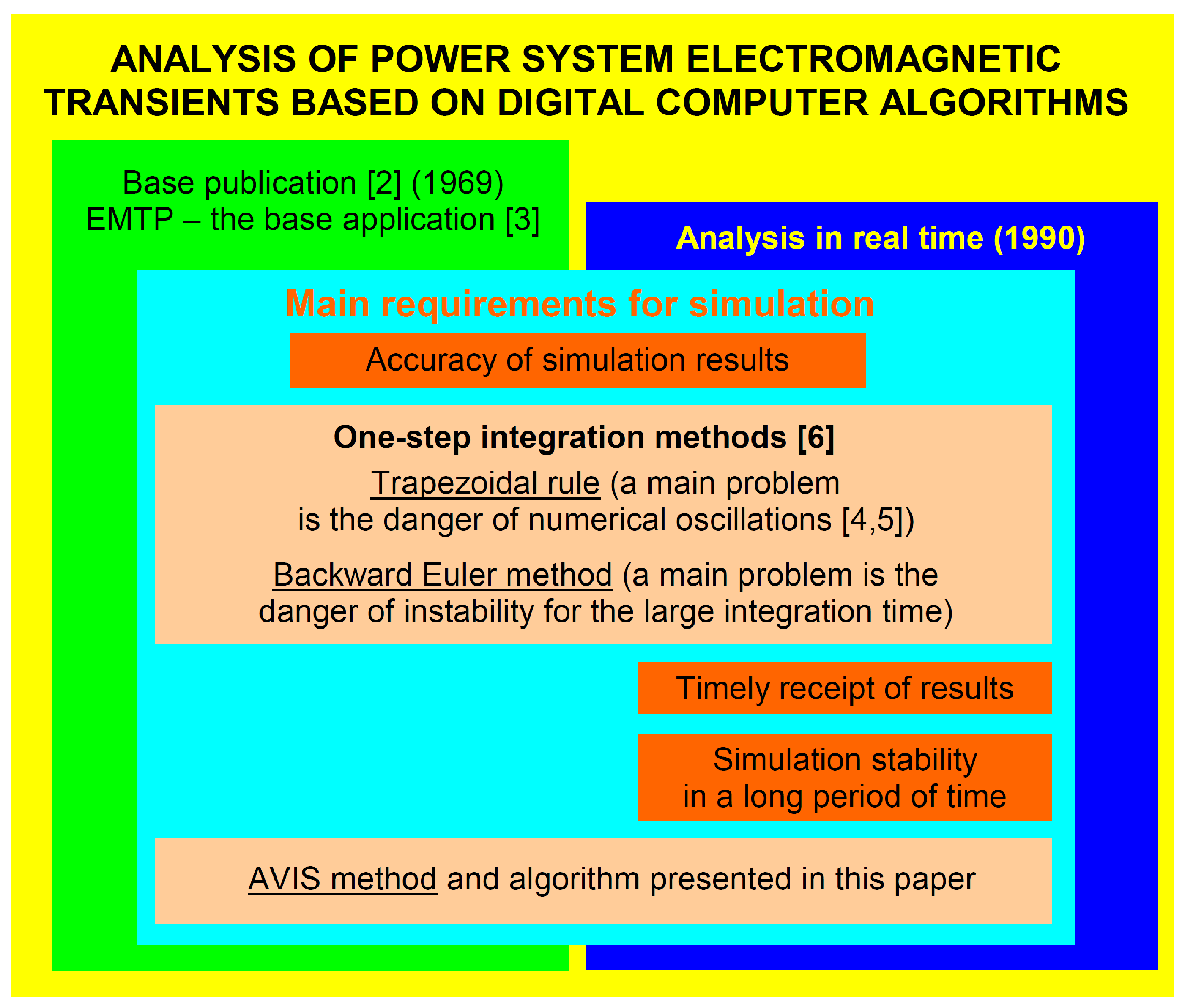
The application of efficient computational techniques to the solution of electromagnetic transient problems in systems of any size and topology is the actual scientific problem. The electric power system variables are continuous. The digital simulation is of course discrete. The main task in digital simulation is still the development of suitable methods for the solution of the differential and algebraic equations at discrete points. The diagram presented in Figure 1 shows the place of one-step integration methods in the analysis of the dynamics of electrical systems. The following publications were listed there: basic Dommel’s book [2], EMTP Theory Book [3], Araujo’s Ph.D. thesis [4], Marti’s publication [5] and Crow’s book [6].
The selection of an integration method and an algorithm is, in particular for the real-time mathematical modeling, an important and current scientific problem. The integration method for real-time simulation must be numerically stable, computationally efficient, and accurate enough for practical purposes.
The book [7] can be distinguished especially in the area of the parallel calculation in the real-time simulation of power system dynamics. The book [8] has a chapter on real-time simulation. A number of Ph.D. Thesis on real-time simulation were carried out, including [9,10,11].
The use of parallel calculations can significantly reduce the computation time. It is especially important in the case of real-time simulation and also simulation realized faster than real time (for example, the prediction of power system operating states). Real-time systems are widely used in the simulation of complex electric circuits [12]. In these kinds of systems, calculations for the given iteration of the discrete mathematical model of electrical system have to be done in the given integration time step [13]. This is an indispensable condition to be met with the requirements related to operation in real-time. Extracting individual processes is not a trivial problem. This subject in relation to electrical systems has been discussed in the literature. Methods such as wave relaxation [14] and domain decomposition [15,16] were used here. The main issue that occurs in the first case is the lack of guaranteed convergence for a general electric circuit. This caused the inhibition of using this method in simulating software of electrical systems. Scalability for algorithms based on the domain decomposition method is strictly limited in the case of increasing numbers of interface variables between extracted parts of the equation system [17].
The explanation of the parallelization of long-running power system simulations using existing desktop computer technology is presented in the book [7]. The topic of partitioning and evaluating runtime as a power system model with partitioned numerous times was discussed in this book. This book provides a fresh perspective on power system simulation to embrace multicore technology, including, among others: the power system model, time domain simulation, discretization, power apparatus models, network formulation, partitioning, and multithreading. In the topic of interest to us, from the point of view of this paper, tunable integration and root-matching were used in the book [7]. Tunable integration was used for stand-alone electrical branches and control blocks, and root-matching was used for electrical branch pairs. Let us pay attention to a certain context of the solution proposed in this book. The choice of integration method typically depends on which power apparatus is included in the model. For example, the trapezoidal rule is recommended for networks where the voltages and currents are expected to be sinusoidal; the backward Euler method is recommended for networks where the voltages and currents are expected to be piecewise linear such as when power converters are present. Tunable integration was defined in [8], and it is an effective approach that benefits from the accuracy of trapezoidal integration and the stability of backward Euler integration. Therefore, it is expedient to look for new integration methods that will avoid the use of the tunable integration.
The answer to these problems is the new numerical one-step integration method and the resulting new mathematical models and new simulation algorithms that are used in the research carried out at the Institute of Electrical Engineering UTP University of Science and Technology in Bydgoszcz (Poland). Previously, no one wrote about this method, mathematical models, and algorithms in any of the above-mentioned publications. The essence of the new method is the use of the numerical discretization of electrical circuit equations, formulated for average voltage values [18]. The proposed method was successfully developed and used by the authors from IEE UTP for issues related to the analysis of complex power systems [19,20,21,22]. A survey of power systems analysis programs presented above did not mention the method based on average voltages in the integration step (AVIS method) even once.
The goal of this paper was the presentation of the scientifically acceptable general method for the mathematical modeling of the dynamics of linear electrical systems using parallel calculations. The new method for the mathematical modeling has an advantage over others known from the literature in that it allows for a stable simulation with a relatively large integration time step without losing the accuracy of the results. The original contributions of the author of this paper were the method of determining the areas of application of the proposed integration method, in which it has an advantage over other methods and the theory of mathematical modeling of dynamics of linear electrical systems using parallel calculations.
The organization of the article is as follows: (1) we present in detail the derivation and physical basis of the mathematical models of individual structural elements and the mathematical model of the generalized electrical system; (2) we present the method of separating the fragments of the mathematical model of the generalized electrical system into computational threads that can be implemented in parallel; and (3) we present, on a relatively simple example, the application of the mathematical modeling method proposed in this paper.
Section 1 of this paper presents the Introduction, which justifies the need to search for effective methods of the mathematical modeling of complex electrical systems, especially those that are to be used in real-time simulators. It has been shown that not everything is solved today in the area of the real-time simulation of the dynamics of power systems. The search for new stable simulation methods with a relatively large integration time step without losing the accuracy of the results is a current issue from the scientific point of view. The ability to perform computations in parallel is a way to speed up computation as expected in a real-time simulation. Section 2 defines the generalized electrical system and provides the basic terms and definitions used in the proposed method for the mathematical modeling of electrical systems. Mathematical relationships between physical quantities characteristic of a generalized electrical system are also presented. The mathematical model of the generalized branch of the electric circuit, based on the AVIS method, is presented in Section 3. The mathematical model of the generalized branch of the electric circuit was used to create mathematical models of the interconnecting structural elements, in which the terminals of the branches extend outside the structural element (a multi-term element). The advantage of the applied integration method (AVIS method) over others (backward Euler and trapezoidal rule) recommended in the literature is demonstrated in Section 4. The derivation and physical justification of the mathematical models of structural elements with any internal structure are presented in Section 5. The mathematical basis for aggregating three structural elements into one equivalent element is presented in the Section 6. This is an example of the aggregation of multiple structural elements for which the external characteristics are known (the internal structure of the element does not have to be known) into one equivalent structural element. This manner is often used in modeling complex power structures. The mathematical bases and physical justifications presented in Section 2, Section 3, Section 5, and Section 6 form the basis of the formulation of the algorithm of the mathematical modeling of linear electrical systems with parallel calculations. This algorithm is presented in Section 7. In Section 8, on a very simple example, the practical application of the algorithm resulting from the method proposed in this paper is shown. The conclusions are at the end of the paper.
The paper does not provide the implementation of the proposed method in a specific hardware solution of the simulator. A detailed description of the implementation of the proposed mathematical modeling method of electrical systems, due to its specificity (PC, DSP, FPGA, GPU), is beyond the scope of this paper.
2. Basic Terms and Definitions
The concept of a generalized electrical system is introduced here. Any electrical system consists of all of the elements needed to generate, distribute, and consume electrical energy. This system can be simplified as shown in Figure 2.
Definition 1.
A generalized electrical system is an abstract object, consisting of abstract elements, that is characterized by suitable physical (electrical) and mathematically exact relationships among these elements.
The word “abstract” is understood in the sense of being a product of abstraction. That is, extracting characteristics or relations, i.e., formal relationships in a real object or event, or in a set of objects or events.
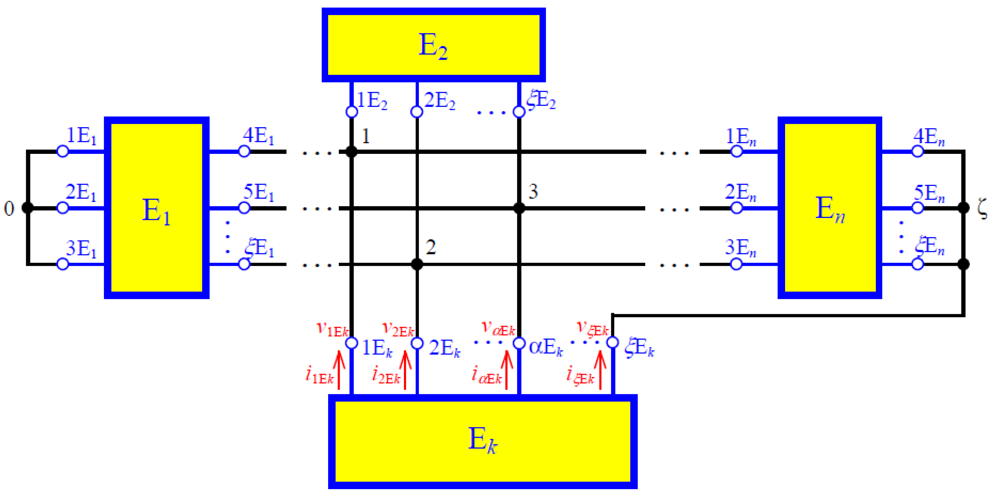
Generalized electrical system can be interpreted as the connection of n multi-terminal elements in + 1 nodes (0, 1, 2, 3, …, ), as shown for example in Figure 2.
Physical (electrical) relationships, resulting directly from Definition 1, imply identifying physical quantities characteristic of nodes (black points in Figure 2) of this generalized electrical system as electric potentials. An electric potential of one of the nodes is taken as a reference (). Based on that, it is possible to introduce the vector of node electric potentials of the generalized electrical system, as follows:
where is the vector of the node electric potentials of the generalized electrical system, is the electric potential of node x (where: x = 1, 2, 3, …, ), and the symbol “T” in the superscript of the matrix notation means the transposition operation.
The essence of the new method of the integration of differential equations, which will be presented in detail in the next section, is to write down the equations for the average voltages in the integration step. Hence, in the mathematical models, the matrix of average electric potentials is used. Thus, the vector of average electric potentials in the integration step h for discrete time has the following form:
where is the average electric potentials in the integration step of node x (where: x = 1, 2, 3, …, and ).
Electrical systems naturally consist of separate multi-terminal elements interconnected with each other. Alternatively, it is also possible to carry out artificial extraction (decomposition) of the electrical system on the separate elements. Separate elements can be called structural elements of the analyzed electrical system (structural elements).
Definition 2.
The poles of each separate multi-terminal element (structural element) are the terminals (nodes) of this element that are available outside and allow direct electrical connection with other elements.
These multi-terminal elements (structural elements) are known from electrical circuit theory as electric multipoles. Multipoles are introduced as elements with ordered external terminals (poles) consisting of a network and a family of terminal classes. The terminal classes are disjoint subsets of the node set of the corresponding network [23]. The rest of the nodes (after extraction of poles) in the structure of each structural element are named internal nodes of this element. Each structural element in the general case is composed of g number of branches that are interconnected with each other. The branch is a set of interconnected ideal elements of electric circuits, which has only two terminals on the outside. Branches of the structural element are interconnected in Ek number of poles (see Figure 2) and w number of internal nodes. Two vectors of external physical quantities are introduced for each structural element , as follows:
where and are the vectors of the node (pole) potentials and currents of the external branches of structural element (current directions in external branches of the structural elements are always oriented from inside the elements to the poles) and and are the electric potential of pole x and the current of the branch with pole x (where x = 1, 2, …, , …, ) of structural element Ek (see Figure 2), respectively.
We consistently introduce the vector of average electric potentials of poles of structural element in the integration step for discrete time , as follows:
where is the average electric potentials in the integration step of pole x of structural element Ek (where: x = 1, 2, …, , …, ).
Definition 3.
The external equation of the structural element is an equation in the following form (formulated for element ):
Equation (6) is composed of matrices for which is a square matrix of size and is the column matrix with number of elements. Those matrices are described by parameters and physical quantities, which occur inside structural element . The methods of the calculations of those matrices elements are introduced in next parts of this paper.
Dependencies between the pole potentials of structural element and the nodal potentials of the analyzed electric system are described by equation:
where is the incidence matrix of structural element .
The same relationship is valid for the average pole potentials of the structural element (Equation (5)) and the average nodal potentials of the analyzed electric system (Equation (2)), as follows:
Definition 4.
The incidence matrix of the structural element is a matrix in which the number of rows is equal to the number (ζ) of independent nodes of the generalized electrical system and the column number is equal to the number (ξ) of poles of this structural element. The matrix element upon crossing the individual row and individual column is equal to one if the node with the number the same as the number of the row is connected to the pole with the number the same as the column number. In other cases, the matrix element is equal to zero.
Based on Kirchhoff’s current law for all independent nodes of the generalized system, the equation was obtained:
Substituting vectors of external branches’ currents determined from Equation (6) for each structural element into Equation (9) and taking into account Equation (8), we obtained the equation:
where:
From Equation (11), it follows that the size of the matrix is , and matrix has number of elements.
Taking into account Definition 2, which is related to the poles of structural element , for the internal nodes (1, 2, …, w) of this element, a vector of internal nodal potentials is written in the form of:
where is the vector of internal nodes potentials of structural element (the symbol “i” indicates that it is about the internal value of the element) and is an electric potential of internal node x (where: x = 1, 2, …, w) of structural element .
We consistently introduce for the internal nodes (1, 2, …, w) of structural element a vector of internal nodal average potentials, in the following form:
where is the average electric potentials in the integration step of internal node x (where: x = 1, 2, …, w).
For each branch (g) of structural element , the branch’s voltages (as the differences of the electric potentials of the respective nodes of the branch) are written in the following vector:
where is the vector of the branch’s voltages of structural element (the symbol “b” indicates that it is about the branches of the element) and is a voltage of branch x (where: x = 1, 2, …, g) of structural element .
We consistently introduce for each branch (g) of structural element the branch’s average voltages in integration step (as the differences of the average electric potentials of the respective nodes of the branch) the following form:
where is the branch’s average voltages in integration step of branches x (where: x = 1, 2, 3, …, g).
The relation between the vector of branch voltages (14) and the vector of internal nodal potentials (12), as well as the vector potential of poles (3) of structural element is given in the following equation:
where is the incidence matrix for internal nodes of structural element and is the incidence matrix for poles of structural element .
The same relationship is valid for average voltages and electric potentials in the integration step, as follows:
Definition 5.
The incidence matrix for internal nodes of the structural element is a matrix in which the number of rows is equal to the number of internal nodes (w) and the column number is equal to the number of its branches (g). The matrix element in the n-th row and the m-th column is equal to: 0 if the terminals of the m-th branch are not connected with the n-th node, or −1 if the terminal of the m-th branch to which the branch current is supplied is connected to the n-th node, or 1 if the terminal of the m-th branch, from which the branch current flows, is connected to the n-th node.
Definition 6.
The incidence matrix for poles of the structural element is a matrix in which the number of rows is equal to the number of poles (ξk) and the column number is equal to the number of its branches (g). The matrix element in the n-th row and the m-th column is equal to: 0 if the terminal of the m-th branch is not connected with the n-th pole, or −1 if the terminal of the m-th branch to which the branch current is supplied is connected to the n-th pole, or 1 if the terminal of the m-th branch, from which the branch current flows, is connected to the n-th pole.
Similar to the case of branch average voltages (15), also for each branch (g) of structural element , branch currents are written in the following vector:
where is the vector of the branch currents of structural element (the symbol “b” indicates that it is about the branches of the element) and is a current of branch x (where: x = 1, 2, …, g) of structural element .
Therefore, for structural element treated as an element of the generalized electric system, we can write the following matrix equations:
Formula (21) is a characteristic of the individual branches as a vector relationship between current and average voltage.
Definition 7.
The solution of the state equation system of structural element is a set of values of the following vectors: , , and , which meets all of the equations and describes the state of this structural element at given excitations, in this case the average values of the potentials of the poles of this element (matrix ).
Definition 8.
The structural element, the branches of which are described by the linear current–average voltage characteristic (21), is the linear structural element.
3. External Equation of the Generalized Linear Branch (Associated with the AVIS Method)
The generalized linear -th branch of the electric circuit of the k-th structural element is treated as a set of ideal elements connected with each other: independent voltage source, independent current source, inductor, resistor, and capacitor. Outside of this set, only two terminals are available (Figure 3).
Resistance of the resistor, inductance of the inductor, and capacitance of the capacitor are known. The source values of and are given in the forms of known analytical functions, e.g., in the following sinusoidal forms:
where amplitudes , , initial phases , , and pulsation are known.
Based on [18] (for m = 1), for the -th branch of the k-th structural element, we can write the current–average voltage characteristics of the generalized linear branch, as follows:
where:
and
4. Accuracy of the Integration Rules
The formulas for the AVIS method, presented in Section 3, and the commonly known formulas for the backward Euler and trapezoidal methods are the basis for assessing the accuracy of these integration methods. It should be noted here that we were interested in the integration methods proposed for real-time simulation. Therefore, many different integration methods used in the general approach to mathematical modeling of electrical systems were omitted here (this will be the subject of other publications).
For the purposes of this paper, the accuracy of an integration rule was assessed by considering its frequency response [3,5,9,24]. The frequency response of the integration for three rules in the discrete-time system H(z) was compared with the exact frequency response of an integrator in the continuous-time system H(s). Additionally, the results of the frequency responses comparison are illustrated with example waveforms for the selected branch of the electrical circuit.
For example, we considered the branch consisting of the following elements connected in series: a resistor, an inductor, and a capacitor, with the known parameters, respectively: resistance R, inductance L, and capacitance C. The branch was powered by a sinusoidal voltage source . Taking the supplying voltage as the input and the current as the output, H(z) is the transfer function of the discrete time system, where (h is integration time step). Applying the above-mentioned three numerical integration methods to the integrator, appropriate transfer functions H(z) were determined, which are listed in Table 1.
The transfer function H(s) of the consideration continuous-time system equals .
Figure 4 and Figure 5 show the accuracy as a function of frequency for the integration rules in Table 1 with the parameters presented in Table 2. Two sets of data were adopted, labeled as (1) and (2), respectively. The frequency axis is labeled in units of up to the Nyquist frequency .
The “teeth” visible in the figures appear near the resonance frequencies (531 Hz for the first set and 130 Hz for the second set). The plots in Figure 4 show that the AVIS method gave very accurate magnitude responses for frequencies in the whole considered range. In addition, the AVIS method produced no phase distortion (excluding frequencies close to the resonance frequency for the first data set). This is clearly visible in the plots in Figure 5. The AVIS method was the best for the two sets of parameters considered here.
Figure 6 shows the current waveforms in the considered branch as the simulation results using three methods: backward Euler, trapezoidal, and AVIS, for the two data sets (see Table 2). These results are perfectly illustrated in the plots presented in Figure 4 and Figure 5. For the second data set, it can be seen that the discrete values obtained from the simulation using the AVIS method (Figure 6c,d) coincided very precisely with the exact solution. Very good accuracy was also maintained at a frequency of 150 Hz (Figure 6c), close to the resonance frequency. For the first set, especially near the resonance frequency (Figure 6a), the phase and amplitude shifts in the solution using the AVIS method are visible. However, the results obtained were acceptable in terms of accuracy. Taking into account the proximity of frequency to the resonance frequency, we achieved a satisfactory result when the difference of the simulation result with the exact solution did not exceed 20%. This difference should be determined close to the maximum values. It should be noted here that the most important effect of the real-time simulation near the resonance frequencies was the maintenance of stability. An error value greater than 20% can make the simulation unstable. The other two methods gave much worse results and were unacceptable in the context of real-time simulators.
The results presented in this section show the advantage of the proposed integration method in a real-time simulation over the other two proposed in the literature. Therefore, it is advisable to develop a new approach to the method of the mathematical modeling of the dynamics of linear electrical systems, with the possibility of parallel calculations. This is what is considered and proposed in the following sections of this paper.
5. External Equation of the Linear Electric Structural Element (Associated with the AVIS Rule)
First, an example of a three-phase structural element was considered, the schematic diagram of which is shown in Figure 7. The current–average voltage characteristic (Formula (21)) of this element takes the following form:
where:
It should be noted that matrix (Equation (29)) contains values of individual physical quantities determined for the time (so it is known from the previous integration step or initial conditions) and also values for time , but there are values of voltage sources and current sources that are given by known algebraic equations.
Substitution Equation (17) into Equation (27) gives the following expression:
which substituted into Formula (19) derives the following equation:
By introducing:
Equation (33) was transformed into the following form:
It should be noted that matrix is a nonsingular matrix with dimension . Taking this into account, it is possible to calculate the matrix of internal nodal average voltages of the structural element as follows:
Expression (32) gives the current vector of the internal branches of the structural element, so substitution of (36) into (32) derives the new form of Equation (32):
where:
The Formula (28) is substituted into (20), directly giving external matrix Equation (6) of the structural element in the following form:
Based on the matrices from Equation (6), it has the following form:
The method of determining the external Equation (6) of a linear structural element with a general internal structure can be carried out on the example of a structural element with the schematic diagram shown in Figure 8.
6. External Equation of the Structural Element as the Internal Connection of the Structural Elements with Known External Equations
In the real-time simulation of the operating states of complex electrical systems, it is useful to apply parallel computing in order to speed up the results of the calculations, without degrading the accuracy. The structural element extraction of the complex electrical system and using the previously described mathematical modeling method give the possibility to apply parallel computing in some parts of the computing process. At some stage of the calculations, it is necessary to solve the system of linear Equation (10) for the analyzed electrical system. Matrix in Equation (10) is a sparse matrix for electrical systems with a high number of nodes (). Even that feature does not enable a significant solving speedup of that equation system. This is due to issues with the effective parallelization of the procedure of solving systems of linear equations. The author of this paper proposed on the particular stage of the calculation process the aggregation of some structural elements’ groups. This tends to replace a few structural elements in the given group by one structural element. This gives the opportunity to significantly reduce the electrical system nodes and reduce the number of equations in Equation (10), so it can speed up solving (even if the calculations are carried out sequentially in this part).
It was assumed that the considered electrical system consisted of structural elements for which the external equations of the form (6) were known. In the general case, the internal structures of the structural elements are not known. Due to that, the extraction of the internal branches of the structural elements being a product of aggregation was impossible. In this case, using only the pole average potentials of the aggregated structural elements and the currents of their external branches was required.
The method of determining the external Equation (6) of a linear structural element resulting from the aggregation of three structural elements, for which external equations are known, was considered on the example of a fragment of the electrical system with the schematic diagram shown in Figure 9.
The external equations of aggregated structural elements are known and have the form of Formula (6). The equivalent structural element E (including the aggregation of three , , and structural elements) will have three poles and five internal nodes (Figure 9, right side). The vectors of the pole average potentials and currents of the external branches of the equivalent structural element E have the form of Formulas (5) and (4), respectively.
For five internal nodes (w = 5), based on Formula (13), the vector of average potentials of these nodes is written as:
Formula (17) is written for branch average voltages, and in the aggregation of structural elements, it does not apply, because there is no reason to recognize, e.g., terminals and as terminals of the same branch. In the case of the aggregation of structural elements, the average potentials of their nodes (poles of aggregated structural elements) should be associated with the average potentials of the poles and internal nodes (Equation (44)) of the equivalent structural element, as follows:
where the incidence matrix of internal nodes and the incidence matrix of poles are determined according to Definitions 5 and 6, respectively.
In this case, the vector of currents of the internal branches of the equivalent structural element E have the form:
and taking into account the characteristics of aggregated structural elements, the following equation is obtained:
where:
Substituting Equation (45) into Formula (47), the following formula is obtained:
which, after substitution into Formula (19), gives exactly the same form as Equation (33). Using the same reasoning in the sequence of Formulas (33)–(40), we obtained formulas for matrices appearing in the external equation of the equivalent structural element E.
7. The Algorithm for the Mathematical Modeling of Linear Electrical Systems with Parallel Calculations
The method for the mathematical modeling of linear electrical systems presented above can be used to simulate the operating states of these systems with parallel calculations. This is particularly applicable in real-time simulators. The rest of this paper presents an example algorithm for using the proposed method to analyze a linear electrical system using parallel calculations.
The preparations for the simulation process were as follows:
- Create an equivalent diagram of the modeled electrical system, and determine the values of the parameters of individual system components (in the proposed method, it is an electrical system as defined in Definition 1); determine the initial values of the individual physical quantities;
- In the equivalent scheme, structural elements may already be naturally separated (in terms of circuit theory, they will be electric multi-poles), or these elements should be arbitrarily separated;
- Identify and mark the nodes of the modeled electrical system (nodes in places where structural elements are connected with each other). Chose one of the identified nodes as the reference node. For the other nodes, formulate the vector of average potentials according to Equation (2);
- Determine the values of the incidence matrix of individual structural elements according to Definition 4. Determine the values of the incidence matrix of individual structural elements according to Definitions 5 and 6 (if necessary).
If an electrical system with a fixed structure is considered, but the simulation process assumes changes in parameter values (e.g., change in switch resistance), then it is expedient to determine the values of the elements of the respective matrix and expressions for the case with closed switch resistance and the matrix for the case with open switch resistance (in the algorithm descriptions, these are matrices with the annotation “if necessary”). In the simulation process, appropriate matrices and expressions are used for the same structural element, but appropriate due to the condition of the switch (this speeds up the calculations, as it is not necessary to calculate the values of matrix elements during the simulation). The determined matrices and expressions can be stored in memory in the form of sets, as presented, for example, in Point 0.2 of the algorithm shown in Figure 10. The example algorithm for the computer simulation of the operating states of the electrical system using the proposed method with parallel calculations is shown in Figure 10.
Figure 11 shows an example algorithm for determining constant matrix and constant expressions for structural elements, which are described in Section 3, Section 5 and Section 6 of this paper. It should be noted that the proposed method for the mathematical modeling of linear electrical systems with parallel calculations can be applied to virtually any system with any structure and also using other methods of integrating differential equations.
The next section presents an example of using the proposed method to analyze the operating states of a linear electrical system.
8. The Example of Using the Proposed Method
The application of the method for the mathematical modeling of linear electric systems with parallel calculations proposed in this paper is shown on the example of a fragment of a MV power distribution network with distributed generation in one phase.
The equivalent diagram of the modeled electrical system is shown in Figure 12. The structural element is a substitute voltage source representing the power system, in the form of three independent branches (three phases), consisting of three series-connected ideal elements: voltage source, resistor, and inductor (based on Thevenin’s theorem).
The system nodes, marked in bold by 5, 6, and 7, represent busbars in the MV power substation. The structural element is an equivalent electric power receiver that contains a fragment of the network that is not modeled in detail. The structural element is a representation of a MV power line section that is derived from the power substation (from Busbars 5, 6, and 7). Element represents an unconventional electric power receiver, whose equivalent diagram is shown in Figure 8. The ideal current source in this element represents a single-phase generating unit (as a distributed generation) that uses renewable energy sources (e.g., a series of single-phase PV installations). The structural element is a representation of another section of the medium voltage power line that connects the load with the and loads. Structural elements and are representations of concentrated loads. The parameters of individual structural elements are summarized in Table 3.
Let us apply the algorithm proposed in Section 7 of this paper. The initial conditions are: the current value for each inductor and voltage on each capacitor. Thus, the following vectors are given:
The nodes of the modeled electrical system are marked in Figure 9 in bold: (where = 0). Based on Equation (2), we have:
The potentials of internal nodes, the voltage at branch terminals, and the branch currents for the structural element are identical to the formulas presented in Section 5.
The incidence matrices (based on Definition 6) for poles of individual structural elements , , , , , and are the same. These matrices and incidence matrices (based on Definition 4) for individual structural elements of the modeled electrical system are easy to determine and are not presented here.
Then, the process of mathematical modeling of the states of operation of the analyzed electrical system proceeds in accordance with the algorithms shown in Figure 10 and Figure 11.
Figure 13 presents examples of the simulation results of the analyzed electrical system (where: f = 50.0 Hz and h = 0.2 ms). Figure 13a,b shows the waveforms of the currents of structural element in a transient state caused by switching on (t = 0) of the three-phase supply voltage system. All initial conditions equal zero (all elements of vectors in (50) equal zero). Figure 13a shows the simulation results using the AVIS method and Figure 13b the results using the trapezoidal method. There were clear differences in the accuracy of the results, of course in favor of the AVIS method.
Figure 13c also shows the waveforms of the currents of structural element E1 characterizing a different transient operating state (using the AVIS method only). This state arose as a result of a simultaneous, significant reduction of the parameters values in two phases (L1 and L2) of the structural element (see Table 3). In this case, there was a short circuit (low impedance) between the system nodes: 9, 10, and 12. The short circuit occurred at t = 50 ms and ended at t = 98 ms. This is a kind of transient short circuit. At the end of the short circuit event, all parameters of the analyzed electrical system returned to their pre-short circuit values.
The same results can be obtained using the aggregation of structural elements, as described in Section 6 of this paper, with respect to elements , , and (as equivalent element ; Figure 9) and , , and (as equivalent element ; Figure 9).
The given results for the example system are only to illustrate the mathematical modeling method proposed in this paper. This simple example was deliberately chosen to achieve a clear effect. A detailed analysis of this example is not the subject of this paper.
9. Conclusions
The development of modern real-time applications, in which complex electrical systems are modeled, is possible when finding a compromise between the accuracy and the time for obtaining results. The problem of accelerating the computational process in the simulation of the operating states of complex electrical systems is still valid. One of the interesting solutions is the use of parallel computations, which was also taken into account in the mathematical modeling method presented in this paper. Another important thread in this topic, poorly developed in the literature, is the use of numerical methods to solve differential equations in mathematical models of power systems with a relatively long integration time step. This was the method used in the solution presented in this paper.
This paper proposed the scientifically acceptable general principle offered to the mathematical modeling of linear electrical systems with parallel calculation. The presented method for the mathematical modeling of linear electrical systems is based on the use and appropriate conceptual approach of two methods known from the electrical circuits theory: methods of the analysis of electrical circuits using multi-terminal electrical components and the nodal method. The proposed method allows the distribution of calculations into individual processes that can be carried out in parallel and simultaneously. In this way, the effect of accelerated calculations is obtained while maintaining the accuracy of the results. However, the main advantage over other algorithms is the use of the method based on average voltages in the integration step (AVIS method). The attention was focused on describing an ordered algorithm. However, the evidence of its effective application in the analysis of the dynamics of electric power and electromechanical systems was indicated in the works carried out by the team of authors from the Institute of Electrical Engineering UTP University of Science and Technology in Bydgoszcz (Poland).
The conclusions of the work described in this paper are as follows:
- This article alone presented the scientifically acceptable general principle offered to the mathematical modeling of dynamics of linear electrical systems with parallel computations. Appropriate formulas for mathematical modeling associated with the method of integrating differential equations based on average voltages in the integration step (AVIS method) were derived. The detailed derivation allowed a simple adaptation of the proposed algorithm to various other integration methods (e.g., backward Euler or trapezoidal methods). However, as was shown in this paper, the applied AVIS method gave the best results in the context of accuracy and the stability of operation in the considered cases.
- The advantage of the AVIS method used over the two other methods proposed in the literature was shown on the example of a series RLC connection. Comparing the frequency responses (magnitude and phase) for discrete and continuous (exact solution) values, the applied AVIS method gave the best results. It is necessary to note at this point that this result cannot be generalized to all cases. Even for the same structure of the electrical system, but for different parameters, the effect may be unsatisfactory. This does not diminish the advisability of using the proposed algorithm and the mathematical modeling method, even if it were only about specific cases.
- In the scientific work carried out at the Institute of Electrical Engineering UTP University of Science and Technology in Bydgoszcz (Poland), using the AVIS method, the problems of simulation stability were identified when there were very small capacitances in the analyzed system. In these cases, it usually helps to apply other known integration methods only to those branches of the circuit with these very small capacitances, of course sticking to the basics of the method, i.e., average voltages in the integration step. This thread will be considered in future publications.
- The proposed algorithm also allows for a partial solution to the problem of the inability to perform parallel calculations, e.g., to solve a system of linear equations. The method of the aggregation of structural elements of the analyzed system presented in this paper allows reducing the number of nodes occurring in an explicit manner, and consequently reducing the number of equations in the system that should be solved numerically (sequentially). In this way, the acceleration of the calculations (solutions of the system of equations) was achieved while maintaining the accuracy of the results.
The proposed algorithm has been verified in many works on real-time simulators of the operating states of complex electrical systems, e.g., [11,19,20,21,22]. This method also has interest for other researchers who analyze real-time management problems of complex electrical systems, including issues regarding procedures for the dispatcher switching off MV power lines in electric power deficit states [25] and research on the charging process of electric vehicle batteries [26].
The author is currently preparing a version of the proposed method for the mathematical modeling of the operating states of nonlinear electrical systems with parallel calculations.
Funding
This research received no external funding.
Institutional Review Board Statement
Not applicable.
Informed Consent Statement
Not applicable.
Data Availability Statement
Data available on request to the author.
Conflicts of Interest
The author declares no conflict of interest.
Abbreviations
The following abbreviations are used in this paper:
| AVIS method | The integration method based on average voltages in the integration step |
| EMTP | The ElectroMagnetic Transients Program |
| IEE UTP | Institute of Electrical Engineering UTP University of Science and Technology |
| in Bydgoszcz (Poland) | |
| GPU | Graphics processing unit |
References
- Kron, G. Tensors for Circuits, 2nd ed.; Dover Publications: New York, NY, USA, 1959. [Google Scholar]
- Dommel, H.W. Digital Computer Solution of Electromagnetic Transient in Single- and Multiphase Networks. IEEE Trans. Power Appar. Syst. 1969, 4, 388–399. [Google Scholar] [CrossRef]
- Dommel, H.W. Electromagnetic Transients Program Theory Book; Bonneville Power Administration: Portland, OR, USA, 1995. [Google Scholar]
- Araujo, A.E. Numerical Instabilities in Power System Transient Simulation. Ph.D. Thesis, Faculty of Graduate Studies Electrical Engineering, University of British Columbia, Vancouver, BC, Canada, 1993. [Google Scholar]
- Marti, J.R.; Lin, J. Suppresion of Numerical Oscillations in the EMTP. IEEE Trans. Power Syst. 1989, 2, 739–747. [Google Scholar] [CrossRef]
- Crow, M. Computational Methods for Electric Power System, 3rd ed.; CRC Press: Boca Raton, FL, USA, 2016. [Google Scholar]
- Uriarte, F.M. Multicore Simulation of Power System Transients; The Institution of Engineering and Technology: London, UK, 2013. [Google Scholar]
- Watson, N.R.; Arrillaga, J. Power Systems Electromagnetic Transients Simulation, 1st ed.; The Institution of Engineering and Technology: London, UK, 2003. [Google Scholar]
- Bayoumi, M. An FPGA-Based Real-Time Simulator for the Analysis of Electromagnetic Transients in Electrical Power Systems. Ph.D. Thesis, Department of Electrical and Computer Engineering, University of Toronto, Toronto, ON, Canada, 2009. [Google Scholar]
- Fajfer, M. Concurrent Computing in the Simulation of the Electric Circuit with the Use of DSP. Ph.D. Thesis, Faculty of Electrical Engineering Poznań, University of Technology, Poznań, Poland, 2019. (In Polish). [Google Scholar]
- Kłosowski, Z. Real-Time Simulation of Electric Power Network with Wind Turbine. Ph.D. Thesis, Faculty of Electrical and Control Engineering Gdańsk, University of Technology, Gdańsk, Poland, 2019. (In Polish). [Google Scholar]
- Estrada, L.; Vázquez, N.; Vaquero, J.; de Castro, Á.; Arau, J. Real-Time Hardware in the Loop Simulation Methodology for Power Converters Using LabVIEW FPGA. Energies 2020, 13, 373. [Google Scholar] [CrossRef] [Green Version]
- Faruque, M.O.; Strasser, T.; Lauss, G.; Jalili-Maradi, V.; Forsyth, P.; Dufour, C.; Dinavahi, V.; Monti, A.; Kotsampopoulos, P.; Martinez, J.A.; et al. Real-Time Simulation Technologies for Power Systems Design, Testing and Analysis. IEEE Power Energy Technol. Syst. J. 2015, 2, 63–75. [Google Scholar] [CrossRef]
- White, J.K.; Sangiovanni-Vincentelli, A. Relaxation Techniques for the Simulation of VLSI Circuits; Kluwer: Norwell, MA, USA, 1987. [Google Scholar]
- Cox, P.F.; Burch, R.G.; Hocevar, D.E.; Yang, P.; Epler, B.D. Direct circuit simulation algorithms for parallel processing (VLSI). IEEE Trans. Comput. Aided Des. Integr. Circuits Syst. 1991, 6, 714–725. [Google Scholar] [CrossRef]
- Frohlich, N.; Riess, B.M.; Wever, U.A.; Zheng, Q. A new approach for parallel simulation of VLSI circuits on a transistor level. IEEE Trans. Circuits Syst. I Fundam. Theory Appl. 1998, 6, 601–613. [Google Scholar] [CrossRef]
- Thornquist, H.K.; Keiter, E.R.; Hoekstra, R.J.; Day, D.M.; Boman, E.G. A parallel preconditioning strategy for efficient transistor-level circuit simulation. In Proceedings of the IEEE/ACM International Conference on Computer-Aided Design—Digest of Technical Papers, San Jose, CA, USA, 2–5 November 2009; pp. 410–417. [Google Scholar]
- Plakhtyna, O. Numerical One-Step Method of Electric Circuits Analysis and Its Application in Electromechanical Tasks. Sci. J. Kcharkov Tech. Univ. 2008, 30, 223–225. (In Ukrainian) [Google Scholar]
- Kłosowski, Z.; Cieślik, S. Real-time simulation of power conversion in doubly fed induction machine. Energies 2020, 13, 673. [Google Scholar] [CrossRef] [Green Version]
- Kłosowski, Z.; Cieślik, S. Stability Analysis of Real-Time Simulation of a Power Transformer’s Operating Conditions. Acta Energetica 2018, 35, 31–38. [Google Scholar]
- Plakhtyna, O.; Kutsyk, A. A hybrid model of the electrical power generation system. In Proceedings of the 10th International Conference on Compatibility, Power Electronics and Power Engineering (CPE-POWERENG), Bydgoszcz, Poland, 29 June–1 July 2016; pp. 16–20. [Google Scholar]
- Plakhtyna, O.; Kutsyk, A.; Semeniuk, M. Real-Time Models of Electromechanical Power Systems, Based on the Method of Average Voltages in Integration Step and Their Computer Application. Energies 2020, 13, 2263. [Google Scholar] [CrossRef]
- Reibiger, A. Networks, Multipoles and Multiports. In Proceedings of the Conference: Circuit Theory and Design (ECCTD), Dresden, Germany, 8–12 September 2013. [Google Scholar]
- Liu, J.; Wei, T.; Liu, J.; Wei, Z.; Hou, J.; Xiang, Z. Suppression of Numerical Oscillations in Power System Electromagnetic Transient Simulation via 2S-DIRK Method. In Proceedings of the 2016 IEEE PES Asia-Pacific Power and Energy Conference (APPEEC), Xi’an, China, 25–28 October 2016; pp. 2230–2235. [Google Scholar]
- Bieliński, K.S.; Bieliński, W. Procedures for dispatcher switching off of MV power lines in electric power deficit states (Procedury dyspozytorskiego wyłączania linii średniego napięcia w stanach deficytu mocy). Rynek Energii 2010, 6, 38–45. (In Polish) [Google Scholar]
- Bieliński, K.S.; Młodzikowski, P. Selected results of research on the charging process of electric vehicle batteries (Wybrane wyniki badań przebiegu procesu ładowania akumulatorów pojazdów elektrycznych). Przegląd Elektrotechniczny 2019, 10, 52–55. (In Polish) [Google Scholar]
Figure 1.
The place of one-step integration methods in the analysis of the dynamics of electrical systems.
Figure 1.
The place of one-step integration methods in the analysis of the dynamics of electrical systems.

Figure 2.
Schematic diagram of a generalized electrical system.

Figure 3.
The generalized linear branch of the electric circuit.

Figure 4.
Magnitude ratio of the frequency response of the integration rules (h = 0.2 ms).

Figure 5.
Phase ratio of the frequency response of the integration rules (h = 0.2 ms).

Figure 6.
Current waveforms for different integration rules and for different data sets (according to Table 2).
Figure 6.
Current waveforms for different integration rules and for different data sets (according to Table 2).

Figure 7.
Structural element that reflects the three-phase element consisting of generalized linear branches.
Figure 7.
Structural element that reflects the three-phase element consisting of generalized linear branches.

Figure 8.
Schematic diagram of the internal structure of the example structural element.

Figure 9.
Schematic diagram of a fragment of the electrical system in which structural elements are aggregated and a diagram of the equivalent structural element.
Figure 9.
Schematic diagram of a fragment of the electrical system in which structural elements are aggregated and a diagram of the equivalent structural element.

Figure 10.
The example algorithm for the computer simulation of the operating states of the electrical system using the proposed theory with parallel calculations.
Figure 10.
The example algorithm for the computer simulation of the operating states of the electrical system using the proposed theory with parallel calculations.

Figure 11.
The example algorithm for determining constant matrix and constant expressions for structural elements described in Section 3, Section 5 and Section 6.

Figure 12.
The equivalent diagram of a fragment of a MV power distribution network with distributed generation in one phase.
Figure 12.
The equivalent diagram of a fragment of a MV power distribution network with distributed generation in one phase.

Figure 13.
Waveforms of the currents of the structural element in a transient state caused by switching on of the three-phase supply voltage system ((a) the AVIS method and (b) the trapezoidal rule) and the currents of this structural element during the short circuit ((c) the AVIS method).
Figure 13.
Waveforms of the currents of the structural element in a transient state caused by switching on of the three-phase supply voltage system ((a) the AVIS method and (b) the trapezoidal rule) and the currents of this structural element during the short circuit ((c) the AVIS method).


Table 1.
Discrete-time transfer function H(z) for the integration rules.
| Integration Rule | Transfer Function H(z) |
|---|---|
| Backward Euler | |
| Trapezoidal | |
| AVIS First Order |
Table 2.
Parameters of the considered branch of the electrical circuit.
| Parameter | V | R | L | C |
|---|---|---|---|---|
| Value of parameter (1) | 320 V | 100 Ω | 300 mH | 300 nF |
| Value of parameter (2) | 320 V | 10.0 Ω | 150 mH | 10.0 μF |
Table 3.
Parameters of the structural elements of the modeled electrical system.
| = 2.64 k | = 1.16 | = 1.16 | = 2.62 k | = 2.62 m | = 2.64 k |
| = 2.64 k | = 1.16 | = 1.16 | = 2.62 k | = 2.62 m | = 2.64 k |
| = 2.64 k | = 1.16 | = 1.16 | = 2.62 k | = 2.62 k | = 2.64 k |
| = 3.05 H | = 122 mH | = 120 mH | = 1.05 H | = 10.5 μH | = 8.30 μF |
| = 3.05 H | = 122 mH | = 120 mH | = 1.05 H | = 10.5 μH | = 8.30 μF |
| = 3.05 H | = 122 mH | = 120 mH | = 1.05 H | = 1.05 H | = 8.30 μF |
| = 163 m | = 163 m | = 163 m | = 52.1 mH | = 52.1 mH | = 52.1 mH |
| = 12.3 kV | = 12.3 kV | = 12.3 kV | = 0 rad | rad | rad |
| = 2.02 k | = 2.02 k | = 8.02 k | = 163 m | = 163 m | = 163 m |
| = 14.1 H | = 14.1 H | = 10.8 μF | = 1.20 μF | = 1.20 μF | |
Publisher’s Note: MDPI stays neutral with regard to jurisdictional claims in published maps and institutional affiliations. |
© 2021 by the author. Licensee MDPI, Basel, Switzerland. This article is an open access article distributed under the terms and conditions of the Creative Commons Attribution (CC BY) license (https://creativecommons.org/licenses/by/4.0/).
Share and Cite
MDPI and ACS Style
Cieślik, S. Mathematical Modeling of the Dynamics of Linear Electrical Systems with Parallel Calculations. Energies 2021, 14, 2930. https://0-doi-org.brum.beds.ac.uk/10.3390/en14102930
AMA Style
Cieślik S. Mathematical Modeling of the Dynamics of Linear Electrical Systems with Parallel Calculations. Energies. 2021; 14(10):2930. https://0-doi-org.brum.beds.ac.uk/10.3390/en14102930
Chicago/Turabian StyleCieślik, Sławomir. 2021. "Mathematical Modeling of the Dynamics of Linear Electrical Systems with Parallel Calculations" Energies 14, no. 10: 2930. https://0-doi-org.brum.beds.ac.uk/10.3390/en14102930
Note that from the first issue of 2016, this journal uses article numbers instead of page numbers. See further details here.