High Precision LSTM Model for Short-Time Load Forecasting in Power Systems

Abstract

The paper presents the application of recurrent LSTM neural networks for short-time load forecasting in the Polish Power System (PPS) and a small region of a power system in Central Poland. The objective of the present work was to develop an efficient and accurate method of forecasting the 24-h pattern of power load with a 1-h and 24-h horizon. LSTM showed effectiveness in predicting the irregular trends in time series. The final forecast is estimated using an ensemble consisted of five independent predictions. Numerical experiments proved the superiority of the ensemble above single predictor resulting in a reduction of the MAPE the RMSE error by more than 6% in both forecasting tasks.

1. Introduction

Load forecasting in power systems plays a significant role in system operation, especially concerning economic impact. The management of market purchases/sales, day-ahead outage planning, energy storage management, future energy contracts, power plants maintenance schedule, and so on necessitates knowing about the upcoming demand and needs of the load. The task of load forecasting is very difficult due to several reasons such as daily, weekly, and annual cycle effects, as well as the random usage of appliances by the consumers.

Many different approaches to load forecasting were tried in the past. A good review of such methods is presented in [1]. The developed approaches start from linear ARMA, SARIMA, and ARMAX [2,3] and end on much more advanced nonlinear models based on neural networks [4,5,6,7]. Two types of neural models were exploited the most: the feedforward neural networks, such as multilayer perceptron (MLP), radial basis function network (RBF), support vector machine (SVM), self-organizing neural networks, and recurrent networks, such as Elman structure or presently the long short-term memory (LSTM) networks. Many different types of individual solutions can be combined to form an ensemble of the improved performance [5]. The other aspect in load demand forecasting is a conceptual study on a virtual power plant architecture for the optimal management of distributed energy resources. The paper [8] proposed such an architecture based on a service-oriented approach. However, the most important problem is still to improve the performance of the individual predicting unit applied in forecasting.

Recently the great interest is in the application of deep learning in prediction problems [4,6,9,10,11,12]. An example of such work is the paper by Kuo and Huang [4], which proposed a deep convolutional neural network model for the load forecasting in the coastal area of the USA for the next three days. Another example is the paper [9], showing the application of autoencoder in forecasting the power demand in the Polish Power System (PPS). The very high interest of researchers is an application of the LSTM recurrent neural network in forecasting tasks [6,11,12,13,14]. This is due to the fact that the hourly needs of power demand are closely related to the previous values, and this is naturally embedded by the nature of the recurrent structure of LSTM [12,13]. Kong [10] et al. used the LSTM to forecasting power load to individual residential households, which is very volatile compared to the region of a power system. Jimenez [12] et al., designed a system for load forecasting focusing on demand-side response events. They used the LSTM model for load forecasting and the exponential moving average methods for peak extraction. Zheng [13] et al. applied the LSTM to build a multi-step load prediction model, in which power levels were detailed. Their research proved the effectiveness of spatial granularity for accurate forecasting. The paper [15] analyzed the effect of different dataset cleaning approaches to the Italian industry load for forecasting accuracy using LSTM. The paper [16] introduced the ADAM algorithm which was chosen in the conducted research.

This paper is concerned with the application of the LSTM network to forecasting the 24-h load pattern with a 1-h and 24-h ahead horizon. Two types of power systems will be considered: the small region of the system and the whole country system. The numerical experiments proved a very high accuracy of the forecasting process. The mean absolute percentage error (MAPE) for the whole year prediction is below 1.5% for Polish Power System at very high correlation coefficients between target and predicted values (above 0.98). These results are much better than those obtained at the application of standard feedforward neural network architectures.

2. Data Used in Experiments

The numerical experiments were performed for two types of data. One is the data of the whole country Polish Power System (PPS) and the second database corresponds to a small region of a power system in the country.

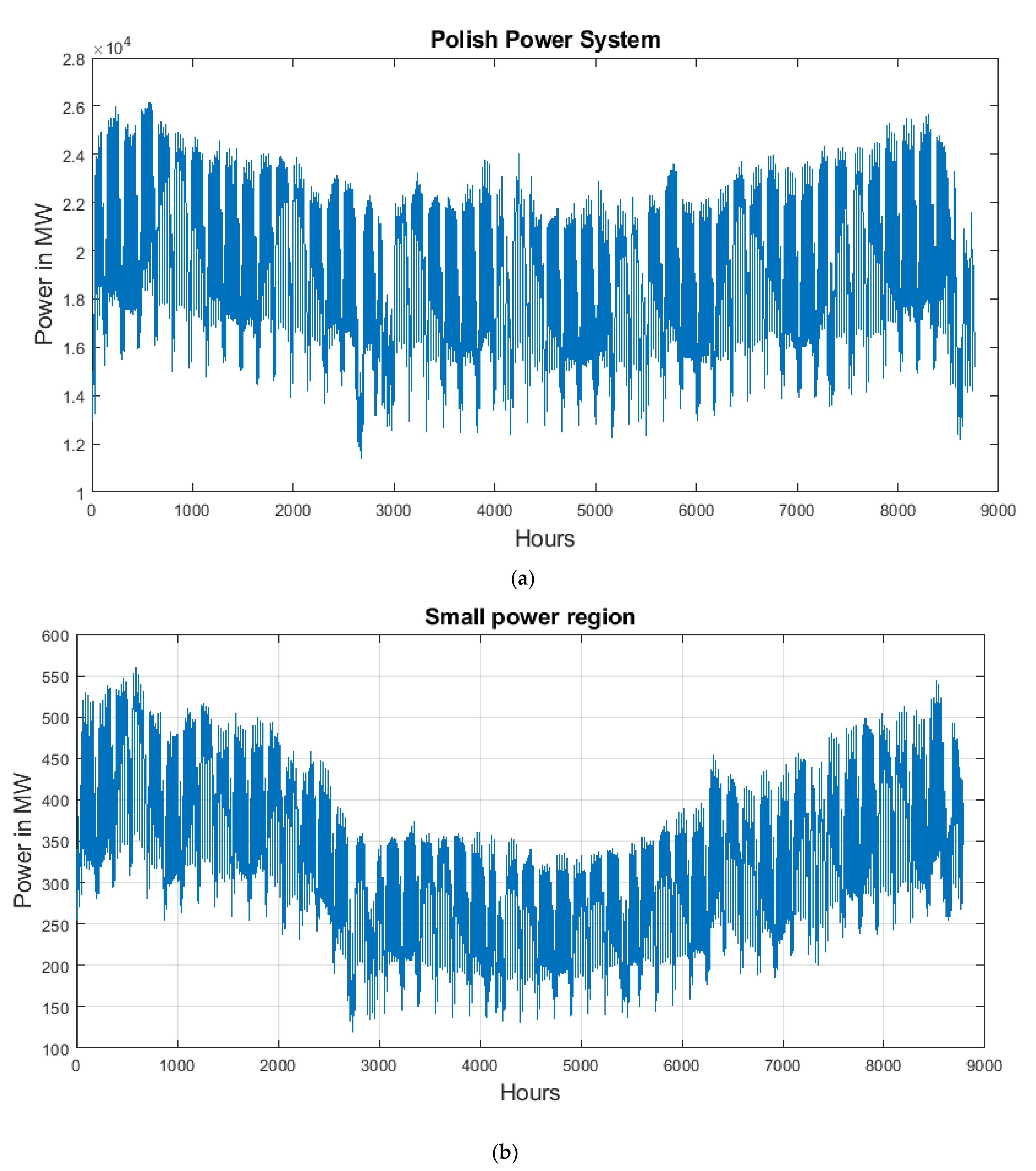
The most important difference is the range of power values as well as the range of changes of powers from hour to hour. This is well illustrated for one chosen year in Figure 1 for both systems.

In the case of the entire PPS, the average demand (in 2019) was 19283.1 MW, and the standard deviation was equal to 3143.1 MW. These values in a small power region are much smaller: average power equal to 378.55 MW and standard deviation equal to 93.38 MW. The difficulty in the prediction task is proportional to the ratio of standard deviation to mean value. The higher this value the more dispersed are the data samples and therefore, more difficult to predict. The coefficient of variation in the case of the considered entire PPS calculated for one year 2019 is equal to 0.1630, while in a small power region this value grows to 0.2467. The earlier experiments on prediction using different types of feedforward neural networks showed mean absolute percentage error (MAPE) significantly higher for small regions. The results presented in this paper will show that the application of recurrent LSTM network is less sensitive to the type of database, achieving good accuracy comparable to both systems and much higher than at application of feedforward predictive systems.

3. Forecasting System Based on Recurrent LSTM Network

3.1. Problem Statement

The general procedure used in forecasting the power demand using the LSTM can be presented as the sequence of the following operations:

•

Take the available time series P(t) of the database and split it into the learning part (P_l(t)) and testing part (P_t(t)).

•

Normalize both data sets using standardization procedure with the mean and standard deviation estimated for known learning data.

•

Apply normalized learning data to the LSTM network and train the network.

•

Freeze parameters of LSTM and test it using the testing data.

•

De-normalize the predicted testing values using the mean and standard deviation values estimated on the learning data. They form the final predicted values.

•

Calculate the quality of the testing results; in the case of not satisfactory results repeat the learning procedure at changed hyperparameters of LSTM.

The standardization procedure is done on both learning and testing data. Each power value corresponding to the hth hour P(h), both learning P_l and testing P_t, is scaled according to the following formula.

$$p(h)=\frac{P(h)-m_l}{s_l}$$

(1)

The mean value m_l = mean(P_l) and standard deviation s_l = std(P_l) are estimated only for learning data P_l and then used directly for testing data P_t, which did not take part in the learning stage. The de-normalization procedure performed on the predicted normalized data p_t(h) is just inverse of the normalization process, i.e.,

$$P_t(h)=p_t(h)\cdot s_l^{}+m_l$$

(2)

Such normalized time series are delivered to the LSTM recurrent predictor. The predictor is learned on the learning samples and the parameters of the network are fixed. Then, the learned LSTM structure is used in the prediction process using the testing data.

Two types of prediction problems were checked. The first one is the task of predicting the 24-h load pattern for the next day. In such a case the learning data are organized in the form of a time series of 24-dimensional vectors directly applied to the LSTM. The second task is to predict the power demand for only one hour ahead. This problem is typical in the very short-term forecasting, frequently used at present in the power market.

3.2. LSTM Time Series Predictor

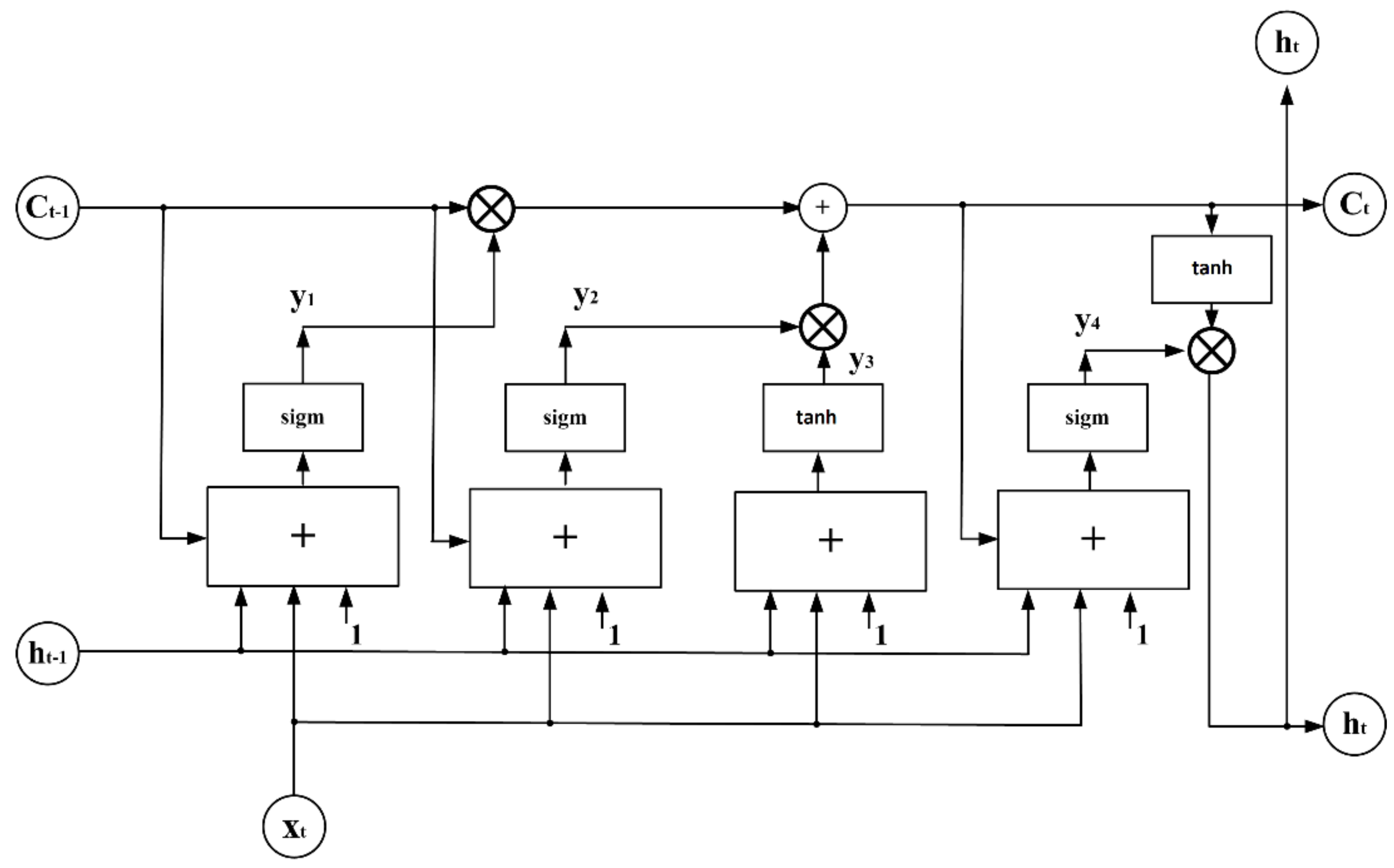
The LSTM developed by Hochreiter and Schmidhuber in 1997 [17,18,19] belongs to the recurrent neural networks. It is composed of an input signal layer, one hidden layer of mutual feedback between neurons represented by so-called LSTM cells. The output layer is fed by the output signals of cells in the hidden layer. The network is composed of many LSTM cells of the general structure presented in Figure 2.

The cell is operating in two succeeding time points: the actual t on its output and the previous t − 1 representing the state of the cell in the previous point of time. The cell performance, denoted by L represents the mathematical function that takes three inputs and generates two outputs,

$$\left(h_t,c_t\right)=L\left(h_{t-1},c_{t-1},x_t\right)$$

(3)

where:

• x_t—vector of input signals in the time points t, representing the actual value of the time series;
• C_t−1—memory signal (cell state) of the cell from the previous time point t − 1;
• h_t−1—output signal of the cell in the preceding time point t − 1.

At the same time, the cell generates two output signals:

• C_t—memory cell state in the actual time points t;
• h_t—output signal of the cell in the actual time point t. This signal of the cell in the hidden layer is delivered to all neurons in the output layer.

Both output signals leave the cell at time point t and are fed back to that same cell at a time t + 1. At any time, the elements of the time sequence x_t are also fed into the cell.

The multiplication gates, denoted by the symbol ×, perform a significant role in cell operation. The upper gate from the left represents the controlled memory. It decides what part of the memory from the previous state is transferred to the actual time. It passes the previous information of the rate from 0 to 1 according to a level of signals y₁. The second gate controls the amount of information c_t, which will form the state of a cell in the actual time point t. The output signal h_t of the cell is created in the right-side multiplicative gate. It is the product of the actual memory signal c_t (after hyperbolic tangential activation) and the output signal y₄ of the sigmoidal neuron supplied by c_t, x_t, h_t−1, and bias. The signal of this gate decides how much information from the past is transmitted to the cell in the next time point.

The structure of the LSTM cell represents a few layers, each characterized by the weight matrices and vectors. Let us assume the notation of them in the form of double indexes: the first one represents the notation of layer signals y_i (here i = 1, 2, 3, and 4) and the second represents the symbol of the input (supply) signal. For example, w_1h represents the weight of the first gate processing the output signals h_t−1 from the previous time point. The sigmoidal function is denoted symbolically by sigm and hyperbolic tangent function—by tanh. In such case, the signals y₁, y₂, y₃, and y₄ are described by:

$$y_1=sigm\left(w_{1c}{c}_{t-1}+w_{1h}{h}_{t-1}+w_{1x}{x}_t+w_{10}\right)$$

(4)

$$y_2=sigm\left(w_{2c}{c}_{t-1}+w_{2h}{h}_{t-1}+w_{2x}{x}_t+w_{20}\right)$$

(5)

$$y_3=tanh\left(w_{3c}{h}_{t-1}+w_{3x}{x}_t+w_{30}\right)$$

(6)

$$y_4=sigm\left(w_{4c}{c}_t+w_{4h}{h}_{t-1}+w_{4x}{x}_t+w_{40}\right)$$

(7)

The actual memory state c_t and the output signal h_t of the cell are described by:

$$c_t=y_2{y}_3+c_{t-1}{y}_1$$

(8)

$$h_t=y_4\cdot tanh(c_t)$$

(9)

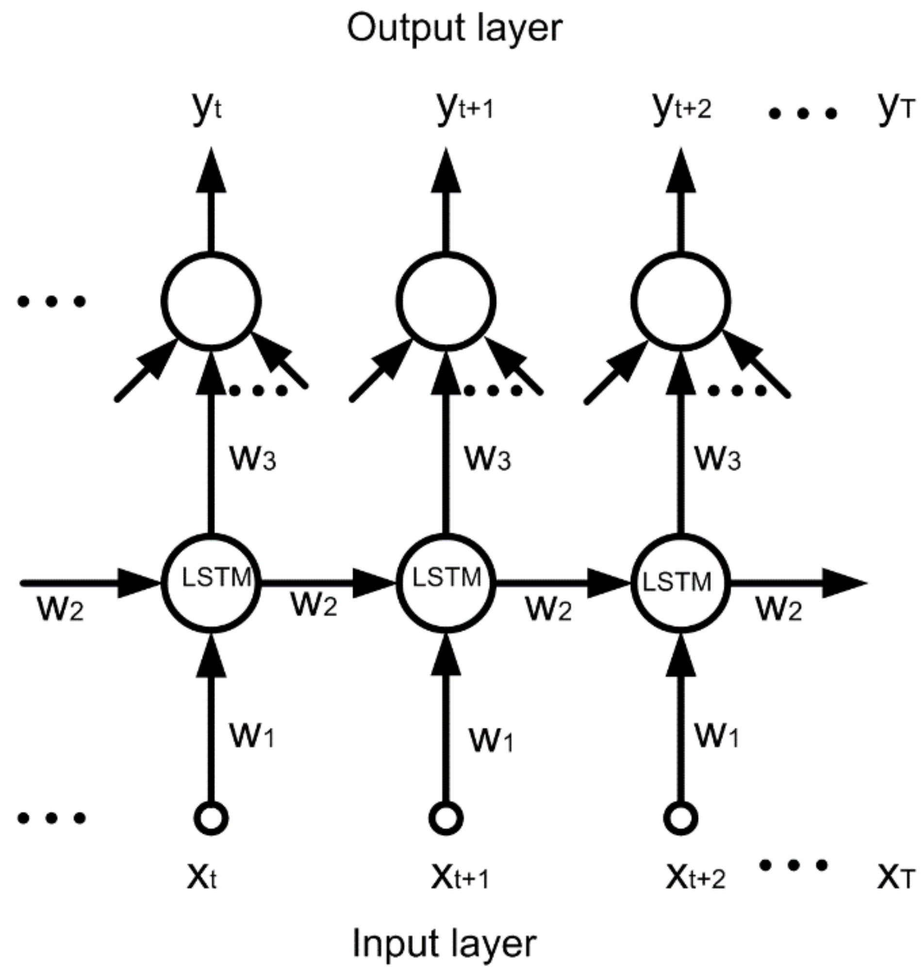
The recurrent operation of the LSTM can be represented as a deep feedforward propagation of signals through time as presented in Figure 3.

The calculation of gradient in the learning procedure is easily implemented in the form of backpropagation through time realized within the assumed time window T, as shown in Figure 3 for one input signal x in different time points: t, t + 1, t + 2,..., T.

The hidden states pass through time; therefore, the recurrent network can take a learning input sequence of any length up to t→T and then can generate an output sequence also of any length. The user decides what is the length of the learning input sequence and what is the length of the output predicted values. The layer of n LSTM cells corresponds to the concatenation of n cells, each with a different set of internal weight parameters. This can be written in a vector form:

$$\left(h_t,c_t\right)=L\left(h_{t-1},c_{t-1},x_t\right)$$

(10)

The individual LSTM weight vectors and biases are stacked into matrices and the elements of these matrices are subject to adaptation in a learning process.

LSTM units are trained in a supervised mode, on a set of training sequences, using a typical gradient descent algorithm, usually with momentum, for example, stochastic gradient descent (SGD) or adaptive moment estimation (ADAM) methods [16]. Tuning the weights needs a set of input-output training pairs. The inputs are fed into the network, pass through the hidden layer to an output and the error between the expected output and the actual output is quantified as a loss function. This error is backpropagated through the network allowing the calculation of the gradient, used in the gradient descent procedure of optimization.

After the model is trained, the next out-of-sample multi-step time series can be produced by the network. At given time series [x_t1, x_t2,..., x_T] we want to forecast the next k time point into the future to achieve [x_T+1, x_T+2, …, x_T+k]. The value k may be just one step producing many-to-one function or many steps producing many-to-many function. Both procedures will be exploited in this paper.

4. Results of Numerical Experiments

Two types of forecasting problems were solved using the LSTM network. The first was to predict the 24-h pattern of the load for the next day, and the second was a one-hour advance prediction. Both types were applied on two different databases: one corresponding to the entire PPS system of the country and the second—to the small region of this power system. The difficulty level of both tasks is very different since the small power region is characterized by much higher changes of load demand from hour to hour.

4.1. Prediction of Load in PPS

The input data delivered to the network is composed of series of 24-dimensional vectors x representing the 24-h patterns of the daily load. Each input vector x(d) of day d is associated in the learning stage with the predicted target vector x(d + 1) of the 24-h load pattern of the next day. The network is trained using the pairs of vectors: input x(d) and output x(d + 1). The training was done using Matlab [20]. After training, the testing data were delivered to the system (none of them were used in the learning phase). In the testing stage, the load pattern for the next day is predicted by the learned network based on the supplied vector of the already known pattern of the previous day. The hyperparameters of the system (number of LSTM cells, number of learning cycles, gradient threshold, initial learning rate, learn rate drop period, and learn rate schedule) were adjusted in the preliminary experiments performed for the 2016 year, which was not taking part in the next experiments. Due to the nature of the recurrent LSTM network structure, in which the predicted pattern is strictly connected with the previous one, the information of the actual season is not significant. Its inclusion has not led to the improvement of the forecasting results.

The structure of the LSTM network used in experiments is 24-n_h-24, where n_h represents the number of LSTM cells. The years subject to an assessment of experiments were: 2017, 2018, and 2019 (2016 was used only in the selection of hyperparameters of the network, fixed in the next experiments). The 24-h load patterns for the next seven days (one week) were predicted at the same time. In the experiments, we assumed that the 24-h loads of the day preceding the prediction, were known (the input pattern to the network composed of the last known day).

The introductory experiments performed in 2016 (not taking part in the next experiments) allowed selecting the best hyperparameters of the network. Different values of hidden neurons (from 300 to 700), initial learning rate in ADAM (from 0.002 to 0.007), learning rate drop factor (from 0.3 to 0.6) were tried in this stage of experiments. The arrangement of the best parameter setting was selected in this way. As a result, the number of hidden neurons was chosen as 600 (for 24-h predicted load pattern), initial learning rate in ADAM 0.005, learning rate drop factor 0.5, and 300 learning cycles were found sufficient.

The analysis of the data showed a highly different pattern of the period of the last 10 days of the year, including the Christmas holiday and the New Year’s Eve. The load pattern in this period is much more chaotic from the day to day and not repeatable. It follows from the fact that most institutions and factories have holidays for some days or work on half-scale on other days. Since the operation of LSTM is sensitive to the shape of learning patterns, we decided to learn two different LSTM models. One was prepared for the first 355 days and the second for the rest 10 days of the year. In the case of 355 days, the first 90% of data were used in learning, and the remaining days (36) for testing in the first experiments. In the case of a network designed for the prognosis of the Christmas holiday period, the population of data are very small. Therefore, the experiments were made including together the data of the last 10 days of the six years (from 2014 to 2019). Six runs of learning and testing were organized in this case. Five-year data (the combinations of five years of data in the period 2014–2019) were used in learning and the remaining year for testing. The experiments were repeated six times for each organization of learning and testing data, and the mean of all testing results is treated as the most representative forecast for this holiday period.

The problem in such organization of experiments is a very small amount of testing data (36 days corresponding to 10% of the yearly data set) representing only one season. Therefore, the next experiments were conducted to assess the performance of the algorithm for the whole year under investigation. The series of experiments were organized in such a way that one-year data (355 days of it) were used for learning and the whole next year’s data were served for testing. In this way, three independent LSTM systems were learned (all of the same architecture and hyperparameters). The first was trained on the data set of 2017 and predicted the daily load for 2018. The second was trained on the data of 2018 and predicted the daily load of 2019. The third system for predicting the load in 2017 used the data set of 2018 in training.

The quality of all results will be demonstrated in the form of MAPE and root mean squared error (RMSE) as well as the correlation coefficient R between the predicted and true values of the load [21]. Their mean values and standard deviations of five repetitions of the learning and testing sessions are presented below. The results of these repetitions are combined into the ensemble and averaged into a single verdict. The results of these experiments for the entire PPS data and three considered years are depicted in

Table 1. Statistical results of numerical experiments in 24-h load pattern prediction in PPS in the case of individual predictors and five repetitions of experiments (testing data cover only 10% of the year).

Year	MAPE (%)	RMSE (MW)	R
2019	1.15 ± 0.11	375 ± 107	0.9952
2018	1.49 ± 0.39	475 ± 69	0.9882
2017	1.13 ± 0.11	373 ± 107	0.9954
Christmas holiday	3.53 ± 0.70	708 ± 136	0.9505

and

Table 2. Statistical results of prediction of 24-h load pattern prediction in PPS of the ensemble composed of five members (testing data cover only 10% of the year).

Year	MAPEensemble (%)	RMSEensemble (MW)	Rensemble
2019	1.10	299	0.9956
2018	1.43	416	0.9916
2017	1.08	293	0.9957
Christmas holiday	3.42	670	0.9552

. Table 1 presents the quality measures averaged over all runs of the algorithm for testing data representing the remaining 10% of the yearly data. For example, the value of MAPE was calculated as the average of all MAPE values in each run, i.e.,

$$MAPE=\frac{1}{5}{\displaystyle \sum }_{i=5}^{5}MAPE\left(i\right)$$

(11)

In the case of an ensemble, the MAPE value of the ensemble is calculated differently,

$$MAP{E}_{ensemble}=\frac{1}{p}{\displaystyle \sum }_{i=1}^p\frac{\left|y_m\left(i\right)-d\left(i\right)\right|}{d\left(i\right)}·100\%$$

(12)

where p represents the number of hours for which the predictions were made, y_m(i) is the mean of values predicted for an ith hour by all members of the ensemble, and d(i) is the true value of the load at the ith hour.

The analysis of the results of different runs of the algorithm showed that in each run the errors (differences between the predicted and true values of load) are of different signs. This opens the space for the compensation of errors in the ensemble composed of the results of the runs. Thanks to the repetitions of the runs and their fusion the quality parameters were improved. This is confirmed by the results shown in Table 2, presenting the MAPE, RMSE, and the correlation coefficient R [21] corresponding to the results of an ensemble composed of five members. The relative ratio of improvement of the ensemble over individual results is in the range of 5%.

The results of experiments covering the whole years in testing (355 days) are shown in

Table 3. Results of numerical experiments in 24-h load pattern prediction in PPS in the case of individual predictors at five repetitions of experiments (testing data cover the whole years, except Christmas period).

Year	MAPE (%)	RMSE (MW)	R
2019	1.37 ± 0.06	2078 ± 178	0.9937
2018	1.65 ± 0.06	2147 ± 136	0.9844
2017	1.56 ± 0.10	2138 ± 100	0.9876

and

Table 4. Numerical results of prediction of 24-h load pattern prediction in PPS of the ensemble composed of five members (testing data cover the whole years, except Christmas period).

Year	MAPEensemble (%)	RMSEensemble (MW)	Rensemble
2019	1.29	305	0.9933
2018	1.59	371	0.9870
2017	1.49	336	0.9882

. They are limited only to the non-Christmas period since the Christmas period results were already presented in Table 1 and Table 2.

This time the results are slightly worse compared to 10% of testing data (for example 1.29% of MAPE compared to 1.10%); however, still of good and acceptable accuracy. Worse results were only for 2017, for which the training data of 2018 were not fully representative.

According to our experience, the best predictive results are obtained when using system learning data corresponding to a long period. Many simulations using data representing different lengths showed that one-year learning data seem to be optimal. However, the important point is the application of the previous year’s period, which immediately precedes the day of the forecast. Thus, in the case of forecasting the load profile for 15 May of the current year, the proposed period used for training should begin in May of the previous year.

The statistical results presented in Table 4 were compared to results obtained for the same PPS in a traditional ensemble composed of multilayer perceptron, radial basis function, and support vector machine cooperating with the autoencoder [9]. The best results of MAPE presented here were given only for 2019. They were at the level of 1.433%, while the LSTM network allowed to reduce this level to 1.29% for the same year. This means that thanks to the application of LSTM the relative improvement of MAPE error is around 10%.

The significant difference in quality measures is visible between the typical days of the year and the Christmas holiday. The Christmas and New Year’s Eve period is very short, and a small amount of learning data is available. Concatenation of five years of data for learning and using the remaining sixth year in testing is still not very representative for the real changes of the load. Moreover, observe that the Christmas period load patterns from different years also differ from each other. This is the reason the prediction errors for this period are much higher.

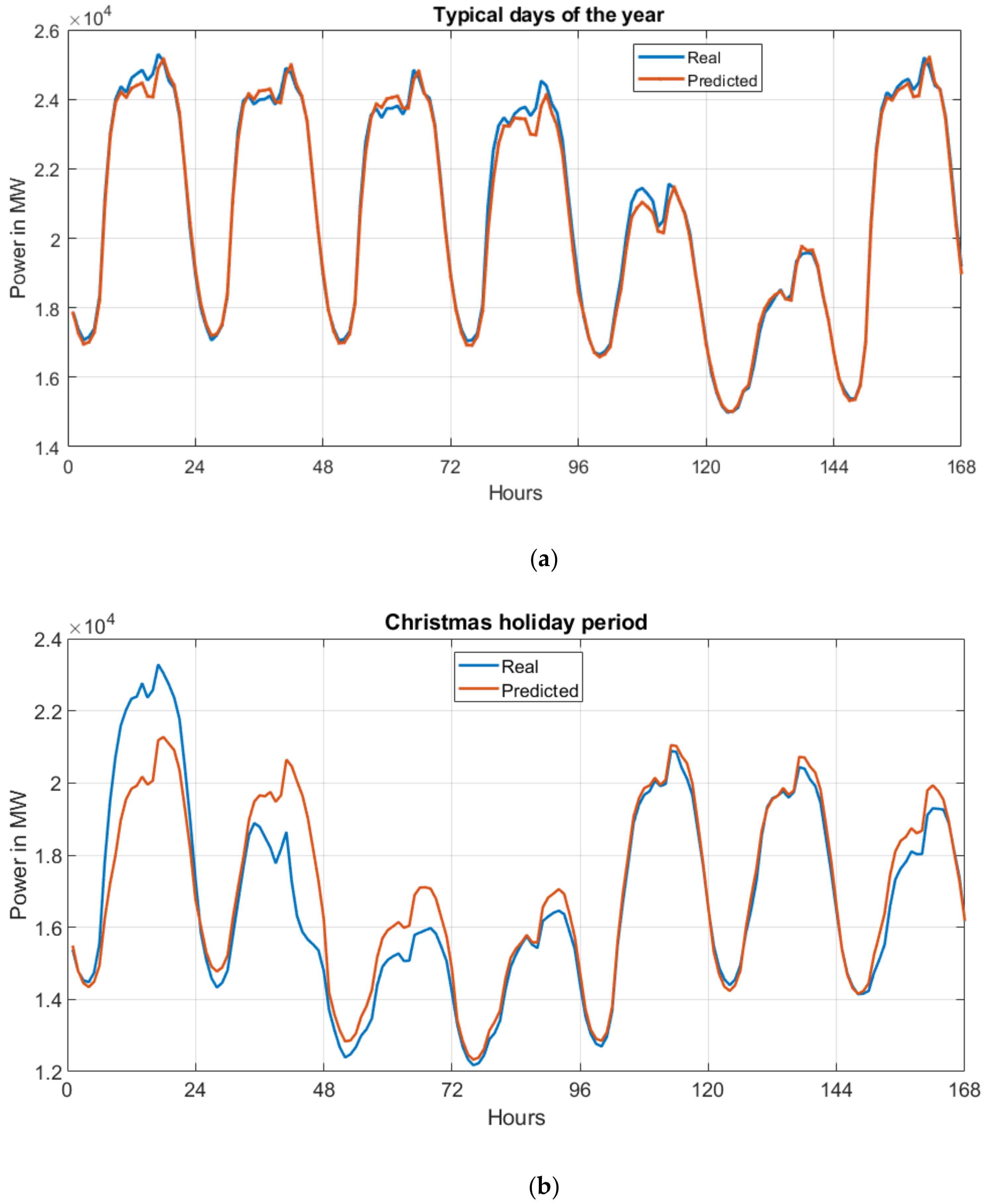
Figure 4 depicts the results of load prediction for one week of the typical days of the year (Figure 4a) and the week corresponding to the Christmas holiday (Figure 4b).

In the case of the typical day, the prediction of the load is close to perfect and the differences between the predicted and true values are negligible and fully acceptable in practice. However, in the case of the not typical period (like the Christmas holiday), the performance of the LSTM predictor is much worse. This is confirmed by the results shown in Figure 4b. Observe that the load of the first 48 hours was predicted based on the last day loads of the Christmas period from the previous year. These days correspond to a New Year’s Eve, usually characterized by the lower consumption of power. Hence, the predicted values for the first two days were underestimated. However, thanks to the available prior information of the past values of load, the LSTM network was able to update these values and performs quite well in the next hours.

The next experiments were performed for a 1-h ahead load pattern for the same time series representing the years 2017–2019. This time the considered load pattern, observed from hour to hour is significantly simpler than for the 24-h treated as one vector. The changes of load from hour to hour are much lower and easier to predict. Moreover, special days of the year (for example Christmas and New Year period) represent now a similar level of difficulty. Therefore, there is no need to build a special network devoted only to them. Once again, we trained the LSTM network using the data of one whole year and tested it on the other one. The years used in learning and testing were organized in the same way as for the whole PPS system. The structure of the proposed network is now 1-n_h-1, with the adjusted n_h = 300. The results will be presented only for testing data of the whole year (data not taking part in learning). Five repetitions of experiments generated the average values of the quality parameters depicted in

Table 5. Statistical results of numerical experiments in 1-h ahead load prediction in PPS in the case of individual predictors at five repetitions of experiments (the results of forecasting the load patterns are shown for the whole tested years).

Year	MAPE (%)	RMSE (MW)	R
2019	1.08 ± 0.03	286.99 ± 12.06	0.9959
2018	0.94 ± 0.04	251.82 ± 9.91	0.9969
2017	1.11 ± 0.02	289.69 ± 6.83	0.9957
Mean	1.04 ± 0.03	276.17 ± 9.60	0.9962

. The interesting conclusion from these experiments is relatively high repeatability results for all days, including such non-typical periods as the Christmas holiday. This is reflected by very small standard deviation values observed in the repetitions of experiments.

After organizing the results of runs in the form of an ensemble the quality factors were improved. Their values obtained for the same testing data are shown in

Table 6. Statistical results of prediction of 1-h ahead load in PPS of the ensemble composed of five members (the results of forecasting the load patterns are shown for the whole tested years).

Year	MAPEensemble (%)	RMSEensemble (MW)	Rensemble
2019	1.03	275.61	0.9962
2018	0.89	239.81	0.9972
2017	1.07	282.85	0.9959
Mean	1.00	266.09	0.9964

.

The relative quality measures (MAPE and RMSE) following from the application of ensemble were increased by almost 4%. The correlation coefficient in all cases was on a very high level, of more than 0.9960. In general, the results show that the LSTM predictor is a very good solution for 1-h ahead load forecasting in PPS.

4.2. Prediction of Load in a Small Power Region

Small power regions experience much larger changes of loads, both in 24-h and 1-h patterns. It was shown in Section 2 in the example of the ratio: standard deviation to mean value. This phenomenon follows from a much higher influence of the individual consumers on the total load. Nevertheless, statistically, the load at a particular hour is more connected with its preceding value. Therefore, the recurrent LSTM network is very well prepared for this forecasting task, due to its nature of the operation.

However, the circuit structure and hyperparameters should be carefully adjusted to the actual task. This was done experimentally using the data of 2016, separately for the 24-h load pattern and the 1-h ahead prediction. In the first case, 600 hidden LSTM units were applied, while in the second case 450 were found the best.

Table 7. Statistical results of numerical experiments in 24-h load pattern prediction in a small power region in the case of individual predictors at five repetitions of experiments (testing data cover only 10% of the year).

Year	MAPE (%)	RMSE (MW)	R
2019	2.22 ± 0.54	17.83 ± 7.64	0.9890
2018	2.66 ± 1.17	19.82 ± 10.59	0.9831
2017	2.26 ± 0.49	11.75 ± 7.80	0.9884
Christmas holiday	4.68 ± 1.37	22.65 ± 7.18	0.9146

and

Table 8. Statistical results of prediction of 24-h load pattern in a small power region of the ensemble composed of five members (testing data cover only 10% of the year).

Year	MAPEensemble (%)	RMSEensemble (MW)	Rensemble
2019	2.14	12.27	0.9896
2018	2.58	14.72	0.9842
2017	2.19	13.12	0.9887
Christmas holiday	4.47	21.68	0.9195

present the results of load prediction for the next day (24-h load pattern). The testing data were limited first to only 10% of the whole year. Table 7 shows the average results of individual five predictors and Table 8—the corresponding results after including these results in the form of ensemble integrated into the averaging mode. At five repetitions of these runs, all quality parameters observed in an ensemble were improved. This is well seen in Table 8, presenting the MAPE, RMSE, and R corresponding to the results of an ensemble.

The next experiments were done for predicting the whole year’s daily patterns (excluding the Christmas period). They were organized for this small power region in the same way as for the whole country. The statistical results of these experiments are presented in

Table 9. Results of numerical experiments in 24-h load pattern prediction in a small power region in the case of individual predictors at five repetitions of experiments (testing data cover the whole years, except Christmas period).

Year	MAPE (%)	RMSE (MW)	R
2019	2.35 ± 0.22	87.12 ± 8.77	0.9872
2018	2.01 ± 0.11	90.72 ± 20.79	0.9958
2017	2.20 ± 0.13	116.44 ± 19.65	0.9934

and

Table 10. Results of prediction of 24-h load pattern in a small power region of the ensemble composed of five members (testing data cover the whole years, except Christmas period).

Year	MAPEensemble (%)	RMSEensemble (MW)	Rensemble
2019	2.12	9.53	0.9929
2018	1.84	7.62	0.9959
2017	2.05	8.29	0.9947

.

The testing results covering the whole years seem to be of better quality. The longer period of testing resulted in improving all measures of quality (smaller MAPE and RMSE and higher value of R). This is well seen by comparing the corresponding values in Table 8 and Table 10.

The next set of experiments was conducted for the prediction of a 1-h ahead load pattern for the time series representing the years 2017–2019. This time the structure of the network is 1-n_h-1, with the adjusted n_h = 450. The experiments were organized in the same way as for the whole PPS system. The results will be given only for testing data of the whole year (they did not take part in learning processes). Five repetitions of experiments showed the average values of the quality measures depicted in

Table 11. Statistical results of numerical experiments in 1-h ahead load prediction in the small power region in the case of individual predictors at five repetitions of experiments (the results of forecasting the load patterns are shown for the whole tested years).

Year	MAPE (%)	RMSE (MW)	R
2019	2.10 ± 0.11	9.91 ± 0.50	0.9943
2018	2.04 ± 0.09	9.77 ± 0.41	0.9947
2017	2.07 ± 0.04	9.36 ± 0.24	0.9949
Mean	2.07 ± 0.08	9.68 ± 0.38	0.9946

.

After applying the ensemble composed of the results of all runs, the quality factors were improved. Their particular values after integrating the results of five runs are shown in

Table 12. Statistical results of prediction of 1-h ahead load in the small power region of the ensemble composed of five members (the results of forecasting the load patterns are shown for the whole tested years).

Year	MAPEensemble (%)	RMSEensemble (MW)	Rensemble
2019	2.01	9.61	0.9946
2018	1.90	9.07	0.9954
2017	1.99	9.12	0.9952
Mean	1.97	9.27	0.9951

.

They correspond well to the results presented in Table 11. With five members of the ensemble, the relative improvement over the mean of the individual members was around 5% for MAPE and RMSE.

5. Conclusions

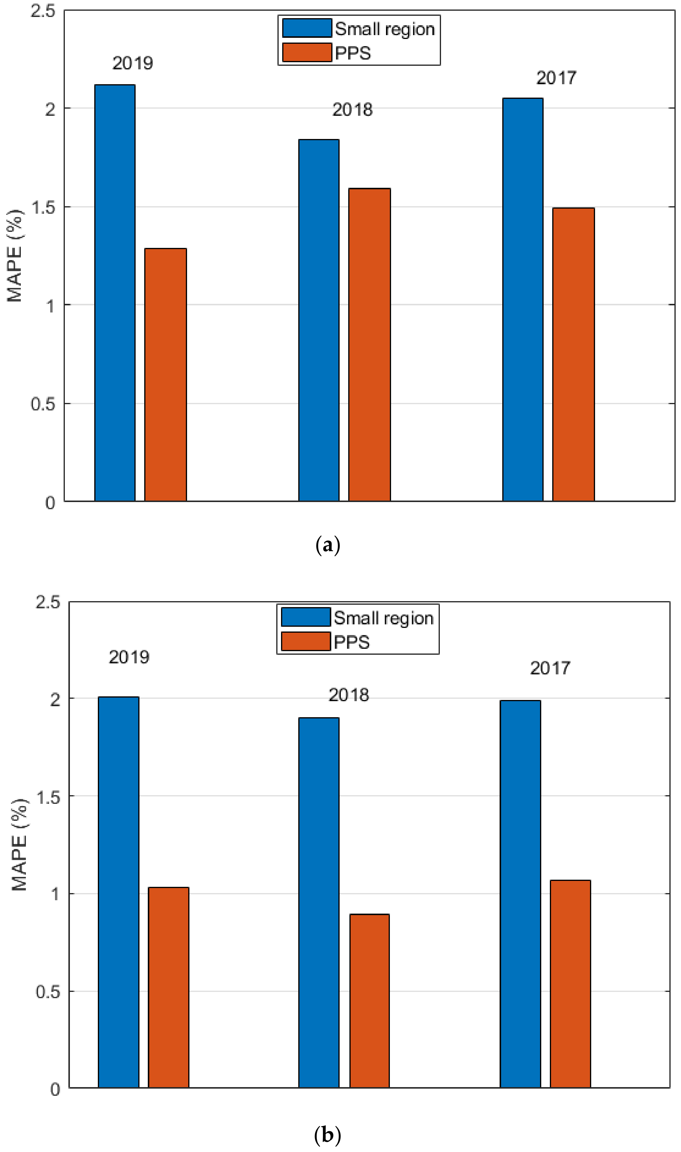
The results of the experiments show the high applicability of the LSTM approach to load forecasting problems in electrical power systems. The recurrent structure of the network allows reproducing very well the trends of changing character of power consumption. However, the accuracy of the prediction depends on the scale of signal variation. This is well illustrated by comparing the MAPE errors in the entire power system of the country (PPS) and the small region of it. The changes and their predictability of power consumption from hour to hour are much higher in a small region, therefore, its forecasting is more difficult. This is well illustrated on the example of MAPE measure in Figure 5. It presents such a comparison in a graphical way for two forecasting problems: prediction of 24-h load pattern (Figure 5a) and 1-h ahead prediction (Figure 5b). Irrespective of the considered year and type of prediction the accuracy obtained in PPS is much higher.

Despite a very simple forecasting model the accuracy of prediction obtained using the LSTM is much better compared to the application of standard feedforward neural predictors. For example, the complex forecasting system based on ensemble applying multilayer perceptron, self-organizing networks, and blind source separation allowed obtaining the MAPE = 1.73% for the PPS. The application of LSTM allowed reducing the mean of errors in three investigated years to the value of MAPE = 1.45% (the days excluding the Christmas period) and 3.42% for 10 days the Christmas period.

The interesting observation from the performed experiments is the high insensitivity of the proposed structure of the LSTM forecasting system to such elements as a type of the season, weather, temperature, etc. The system is based on the strict association of the previous (known) vector and the predicted one. Such relations are well visible in the case of power demand in electrical power systems. Therefore, the proposed solution, despite its simplicity, is very efficient in this task.

References

- Jahan, I.S.; Snasel, V.; Misak, S. Intelligent Systems for Power Load Forecasting: A Study Review. Energies 2020, 13, 6105. [Google Scholar] [CrossRef]
- Herui, C.; Xu, P.; Yupei, M. Electric Load Forecast Using Combined Models with HP Filter-SARIMA and ARMAX Optimized by Regression Analysis Algorithm. Math. Probl. Eng. 2015, 5, 1–14. [Google Scholar] [CrossRef] [Green Version]
- Kim, Y.; Son, H.-G.; Kim, S. Short term electricity load forecasting for institutional buildings. Energy Rep. 2019, 5, 1270–1280. [Google Scholar] [CrossRef]
- Kuo, P.-H.; Huang, C.-J. A High Precision Artificial Neural Networks Model for Short-Term Energy Load Forecasting. Energies 2018, 11, 213. [Google Scholar] [CrossRef] [Green Version]
- Osowski, S.; Siwek, K.; Szupiluk, R. Ensemble Neural Network Approach for Accurate Load Forecasting in the Power System. Appl. Math. Comput. Sci. 2009, 19, 303–315. [Google Scholar]
- Muzaffar, S.; Afshari, A. Short-Term Load Forecasts Using LSTM Networks. Energy Procedia 2019, 158, 2922–2927. [Google Scholar] [CrossRef]
- Wang, L.; Mao, S.; Wilamowski, B. Short-Term Load Forecasting with LSTM Based Ensemble Learning. In Proceedings of the 2019 International Conference on Internet of Things (iThings) and IEEE Green Computing and Communications (GreenCom) and IEEE Cyber, Physical and Social Computing (CPSCom) and IEEE Smart Data (SmartData), Atlanta, GA, USA, 14–17 July 2019; pp. 793–800. [Google Scholar]
- Pasetti, M.; Rinaldi, S.; Manerba, D. A Virtual Power Plant Architecture for the Demand-Side Management of Smart Prosumers. Appl. Sci. 2018, 8, 432. [Google Scholar] [CrossRef] [Green Version]
- Ciechulski, T.; Osowski, S. Deep Learning Approach to Power Demand Forecasting in Polish Power System. Energies 2020, 13, 6154. [Google Scholar] [CrossRef]
- Kong, W.; Dong, Z.Y.; Jia, Y.; Hill, D.J.; Xu, Y.; Zhang, Y. Short-Term Residential Load Forecasting based on LSTM Recur-rent Neural Network. IEEE Trans. Smart Grid 2019, 10, 841–851. [Google Scholar] [CrossRef]
- Kumar, J.; Goomer, R.; Singh, A.K. Long Short Term Memory Recurrent Neural Network (LSTM-RNN) Based Workload Forecasting Model For Cloud Datacenters. Procedia Comput. Sci. 2018, 125, 676–682. [Google Scholar] [CrossRef]
- Jiménez, J.M.; Stokes, L.; Moss, C.; Yang, Q.; Livina, V.N. Modelling energy demand response using long short-term memory neural networks. Energy Effic. 2020, 13, 1263–1280. [Google Scholar] [CrossRef]
- Zheng, Z.; Chen, H.; Luo, X. Spatial granularity analysis on electricity consumption prediction using LSTM recurrent neural network. Energy Procedia 2019, 158, 2713–2718. [Google Scholar] [CrossRef]
- Elsworth, S.; Guttel, S. Time series forecasting using LSTM networks: A symbolic approach. arXiv 2020, arXiv:2003.05672. [Google Scholar]
- Nespoli, A.; Ogliari, E.; Pretto, S.; Gavazzeni, M.; Vigani, S.; Paccanelli, F. Electrical Load Forecast by Means of LSTM: The Impact of Data Quality. Forecasting 2021, 3, 91–101. [Google Scholar] [CrossRef]
- Kingma, D.P.; Ba, J. Adam: A method for stochastic optimization. In Proceedings of the International Conference Learning Representation (ICLR), San Diego, CA, USA, 5–8 May 2015. [Google Scholar]
- Hochreiter, S.; Schmidhuber, J. Long short-term memory. Neural Comput. 1997, 9, 1735–1780. [Google Scholar] [CrossRef] [PubMed]
- Schmidhuber, J. Deep learning in neural networks: An overview. Neural Netw. 2015, 61, 85–117. [Google Scholar] [CrossRef] [PubMed] [Green Version]
- Greff, K.; Srivastava, R.K.; Koutnik, J.; Steunebrink, B.R.; Schmidhuber, J. LSTM: A Search Space Odyssey. IEEE Trans. Neural Netw. Learn. Syst. 2017, 28, 2222–2232. [Google Scholar] [CrossRef] [Green Version]
- Matlab User Manual; MathWorks: Natick, MA, USA, 2020.
- Tan, P.N.; Steinbach, M.; Kumar, V. Introduction to Data Mining; Pearson Education Inc.: Boston, MA, USA, 2013. [Google Scholar]
- Polish Power System Reports. 2021. Available online: https://www.pse.pl/mapa-raportow (accessed on 19 December 2020).
Figure 1.
The hourly changes of the power demands within one year in: (a) entire Polish Power System, (b) small region of a power system.
Figure 2.
The general structure of the single memory LSTM cell. xt is the vector of input signals in the time point t, Ct−1 and Ct represent cell states in the previous t − 1 and actual t time points, ht−1 and ht are output signals of the cell in t − 1 and t time points, respectively, 1 represents the bias. The symbol × represents the multiplication and + summation of signals.
Figure 3.
The scheme of the forward propagation through time representing feedback in the recurrent network. It shows connections of only one hidden neuron (LSTM cell) in a feedforward form at the application of time sequence xt of one input signal x. In backpropagation through time, the direction of the flow of signals is simply reversed and the former output signals are replaced by the actual errors at these points of time.
Figure 4.
The graphical presentation of the real and predicted load patterns for one chosen week: (a) typical days of the year, (b) Christmas period. In the case of the Christmas holiday period higher discrepancy between the true and predicted patterns are visible for the first three starting days of the holiday.
Figure 5.
The comparison of MAPE of load prediction in the entire country (PPS) and in the small power region for the years 2019, 2018, 2017 organized in the mode of (a) 24-h load pattern forecasting, (b) 1-h ahead load prediction. The results confirm the more difficult prediction problem corresponding to a small region.