
A New Method to Determine the Impact of Individual Field Quantities on Cycle-to-Cycle Variations in a Spark-Ignited Gas Engine

1
LEC GmbH, Inffeldgasse 19, 8010 Graz, Austria
2
INNIO Waukesha Gas Engines Inc., 1101 West St. Paul Avenue, Waukesha, WI 53188, USA
*
Author to whom correspondence should be addressed.
Energies 2021, 14(14), 4136; https://0-doi-org.brum.beds.ac.uk/10.3390/en14144136
Submission received: 7 May 2021
/
Revised: 22 June 2021
/
Accepted: 5 July 2021
/
Published: 8 July 2021
(This article belongs to the Special Issue Advances in Spark-Ignition Engines)
Abstract
:Cycle-to-cycle variations (CCV) in spark-ignited (SI) engines impose performance limitations and in the extreme limit can lead to very strong, potentially damaging cycles. Thus, CCV force sub-optimal engine operating conditions. A deeper understanding of CCV is key to enabling control strategies, improving engine design and reducing the negative impact of CCV on engine operation. This paper presents a new simulation strategy which allows investigation of the impact of individual physical quantities (e.g., flow field or turbulence quantities) on CCV separately. As a first step, multi-cycle unsteady Reynolds-averaged Navier–Stokes (uRANS) computational fluid dynamics (CFD) simulations of a spark-ignited natural gas engine are performed. For each cycle, simulation results just prior to each spark timing are taken. Next, simulation results from different cycles are combined: one quantity, e.g., the flow field, is extracted from a snapshot of one given cycle, and all other quantities are taken from a snapshot from a different cycle. Such a combination yields a new snapshot. With the combined snapshot, the simulation is continued until the end of combustion. The results obtained with combined snapshots show that the velocity field seems to have the highest impact on CCV. Turbulence intensity, quantified by the turbulent kinetic energy and turbulent kinetic energy dissipation rate, has a similar value for all snapshots. Thus, their impact on CCV is small compared to the flow field. This novel methodology is very flexible and allows investigation of the sources of CCV which have been difficult to investigate in the past.
1. Introduction
With increasing legislative pressures to reduce reciprocating engine emissions and both governmental and consumer pressures for higher fuel efficiencies, reciprocating engine manufacturers have long been pursuing engine technologies that simultaneously push the envelope of engine performance, efficiency and emissions reductions. For spark-ignited (SI) engines, such pressures have resulted in the development of a wide array air charging and fueling engine technologies that are simultaneously optimized through complex engine control strategies to deliver on one or more aspects of the ultimate goal of highly efficient, high power density, low emissions engines. One of the challenges faced with tailoring the multi-dimensional engine operating envelope is the advanced combustion regimes that are being developed as a part of the overall engine operating recipes tailored to meet these challenges. Use of lean burn combustion and exhaust gas recirculation are two common approaches to improving fuel efficiency while reducing emissions; however, such strategies also introduce significant combustion sensitivities to the in-cylinder physics resulting in combustion regimes which are more susceptible to cycle-to-cycle variation (CCV) as the result of variations the ignition kernel development, kernel growth rates and/or the final fully developed turbulent flame as summarized by the reviews by Young [1], Ozdor et al. [2] and Maurya [3] and extensively noted in experimental studies [3,4,5,6,7,8]. After understanding the causes of CCV, the ultimate goal is the development of control strategies to reduce the magnitude of CCV [9,10,11].
Prior research has well documented the many factors that may promote CCV and these may be categorized as physico-chemical sources—flow field, trapped fuel mass, turbulence, dilution, stoichiometry and fuel reactivity and/or compsition; geometric sources—compression ratio, intake port geometry, spark plug location, spark plug electrode(s) orientation and spark gap; and operational sources—engine speed, load and ignition system performance [1,2,3,4,12,13]. Many of the experimental works quantify CCV by computing the coefficient of variation (CoV) in one or more easily measured metrics including peak cylinder pressure, location of peak firing-pressure, indicated mean effective pressure (IMEP) and/or maximum rate of pressure rise or fuel burning rates with peak cylinder pressure and IMEP being the most common. While these metrics are often easily measured, they tend to lump the many possible driving sources of CCV into a single net contributing factor making it challenging to delineate individual contributions of CCV amongst the possible sources. As a result, recent experimental work has focused on precise measurement of the development of the ignition kernel as the point of 2% of burn fuel mass (MFB2) and kernel growth rate as 0–10% (MFB10) as these two phases of the combustion event tend to be more sensitive to the CCV sources than the fully turbulent flame [5,14,15]. Unfortunately, these metrics are also more prone to measurement error due to the increased level of accuracy required in the cylinder pressure measurement and are complicated by the determination of the cumulative burn mass.
To unravel the complexities associated with the aforementioned strategies for identifying individual sources of CCV in SI engines, researchers have applied a variety of statistical and non-statistical analysis methods of the decomposing measured in-cylinder flow fields into its mean (large-scale) and turbulent (small-scale) components as summarized by Maurya [3] and Sadeghi et al. [16]. The results of such methods are often difficult to interpret from a physical perspective and, as indicated by Sadeghi [16] and Roudnitzky et al. [17], most of the methods invoke ad hoc assumptions that can impact the results of the decomposition, raising questions about the usefulness of such methods.
The early works of Venmorel et al. [18] and Liu et al. [19] and recently the works of Li et al. [20], Richard et. al. [21], Netzer et al. [22] and Truffin et al. [23] have utilized CFD simulation tools to understand the sources of CCV under a variety of engine operating conditions using LES turbulence modeling techniques under the pretense that they may be required in order to resolve the turbulence scales necessary to capture the impacts of turbulent flow field on both early flame kernel development and late stage turbulent flame progression. In their review, Lauer and Frühhaber [24] give an overview of current best practices in science and industry for turbulence modeling in combustion simulations. On the other side, the work of Scarcelli et al. [25] has shown that unsteady RANS (uRANS) turbulence models, with sufficient and practical grid resolutions, can capture many of the driving metrics of CCV in SI engine combustion. Additionally, modifications to the turbulence model used in this paper were proposed in the past [26]. To this end, this work proposes a novel approach for the investigation of the individual contributions of CCV using a detailed uRANS CFD simulation methodology.
2. Materials and Methods
2.1. Engine Setup
The engine used for the simulation is an INNIO Jenbacher natural gas four valve engine with premixed gas–air mixture and roughly 2.4 L of displaced volume. Bore and stroke are 135 mm and 170 mm, respectively. The engine is operated at a speed of 1500 rpm.
2.2. CFD Simulation Setup
The three-dimensional CFD simulations are performed with the CONVERGE CFD solver (version 3.0.13; Convergent Science; Madison, WI, USA). The mesh size in the intake and exhaust ports is 2 mm and 1 mm in the cylinder, respectively. Near-wall refinements and adaptive mesh refinement (AMR) for the flame front is employed, leading to 0.25 mm cells at the flame front location. Turbulence is modeled by the two-equation RANS k- RNG turbulence model. Ignition is modeled by an energy deposition at the spark plug gap of 30 mj each for 0.6 CAD for breakdown phase and 7.6 CAD for arc-glow phase. Combustion is modeled using the detailed chemistry approach and the GRI Mech 3.0 reaction mechanism [27] for natural gas combustion. An adaptive time step marching scheme is used to maintain a maximum Courant–Friedrichs–Lewy (CFL) limit within the domain to 2 during the gas exchange, and 4 during compression, except during combustion, a constant time step of 10−6 s is used resulting in maximum advection and diffusion CFL numbers of less than 1.0. Total pressure and temperature are prescribed at the inlet to the intake port, and static pressure is prescribed at the outlet of the exhaust port. Additionally, turbulence intensity of 2% and a turbulence length scale of 3 mm were specified at the inlet to calculate the boundary conditions for k and .
2.3. Multi-Cycle Simulations
A total of eleven consecutive engine cycles are simulated, using periodic (one engine cycle) boundary conditions with first cycle discarded due to initialization effects. The location and duration of the ignition are not changed. At 5 CAD and 0.5 CAD before spark timing, snapshots of the simulation are saved allowing for simulations to be restarted and/or implementation of the recombination strategy as described in the next section. The uRANS approach is in line with past work to predict CCV of internal combustion engines [28,29,30].
2.4. Combination of Simulation Snapshots
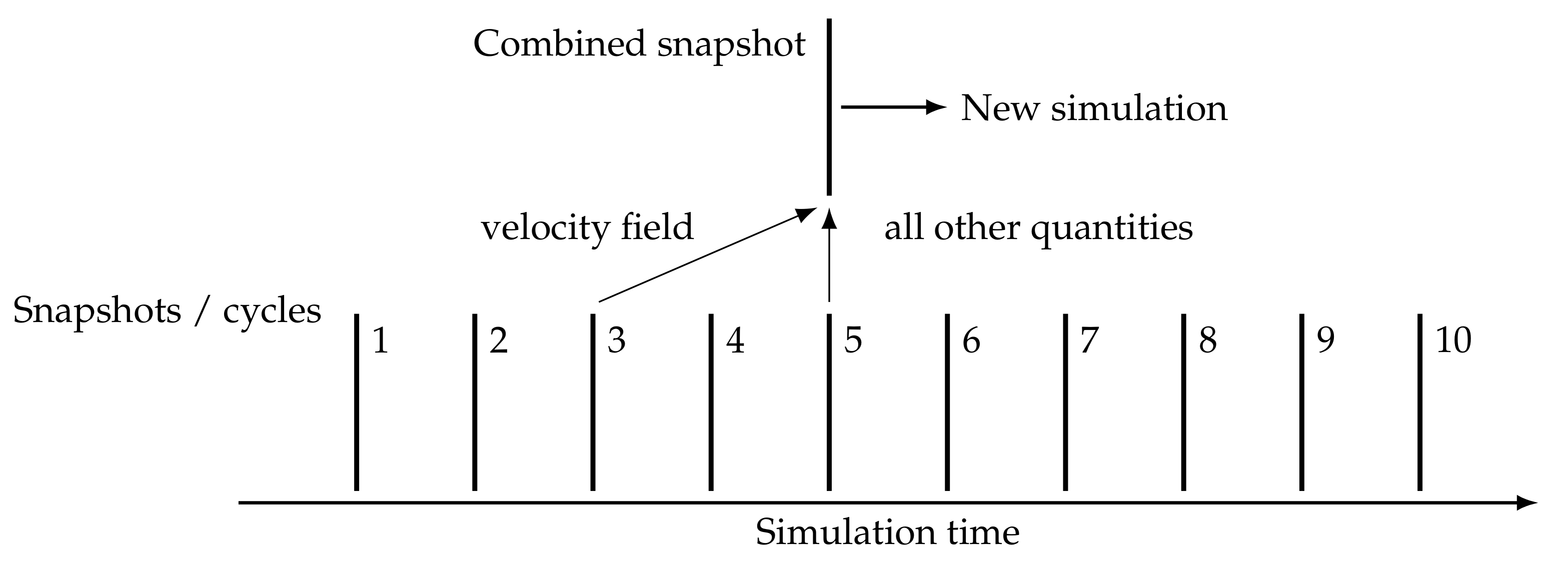
The restart files are a snapshot of the simulation at a certain time and allow one to restart the simulation from this time with minimal or no change in results as shown in Figure A1 and Figure A2. The process of combining fields from different restart files is not supported by the CFD code and therefore a small Python script is used to combine fields from different restart files into a single restart file, a combined snapshot. Figure 1 visualizes the general idea of the recombinations. The restart files are HDF5 files and can be read and edited using standard tools from the h5py [31] Python package.
It should be noted that while restart files (i.e., snapshots) are written at the same crank angle degree before spark timing of each engine cycle and the geometry and position of the piston are exactly the same, the mesh is different as a result of AMR being used to resolve the velocity field during gas scavenging. Thus, the combination algorithm accounts for local variances in mesh resolution combining the fields. For example, starting from a base snapshot where a majority of the instantaneous field quantities will be used without modification, to replace the instantaneous velocity fields with the values from another snapshot, here referred to as the velocity snapshot, the following procedure is applied:
- Extract the mesh data from both the base and velocity snapshot.
- Extract the velocity field from the velocity snapshot.
- Interpolate the velocity field, which is defined on the mesh of the velocity snapshot, onto the mesh of the base snapshot. This is done by looping over all the cells of the base snapshot and finding the value of the velocity field of the cell of the velocity snapshot which is nearest to the cell of the base snapshot.
- Write the newly interpolated field, which is now defined on the mesh of the base snapshot mesh, into the corresponding data array. Thus, the original, base velocity field is replaced with the exchange dataset.
3. Results
Due to confidentiality, all data reported here is normalized: The in-cylinder peak pressures are normalized to the minimum and maximum peak pressure, i.e., a peak pressure of 100% and 0% correspond to the highest and lowest peak pressure, respectively, and the reported absolute crank angle degrees are normalized with respect to the ignition timing, i.e., all reported absolute crank angle degrees in this paper are relative to the ignition.
The multi-cycle uRANS simulation yields ten different in-cylinder pressure traces as shown in Figure 2. The in-cylinder peak pressure has a coefficient of variation of 1.15%. The main differences between the cycles are in the peak-pressure and MFB50%. The differences from cycle to cycle in ignition delay and IMEP are significantly lower and are not considered in the following sections.
To ensure that restarting the simulation does not change the combustion result, a dry run is performed where no datasets were exchanged and the same combustion event is re-run using the restart file. These tests show that no significant difference between results from original and restart simulations existed as shown in Figure A1 and Figure A2 in Appendix A.
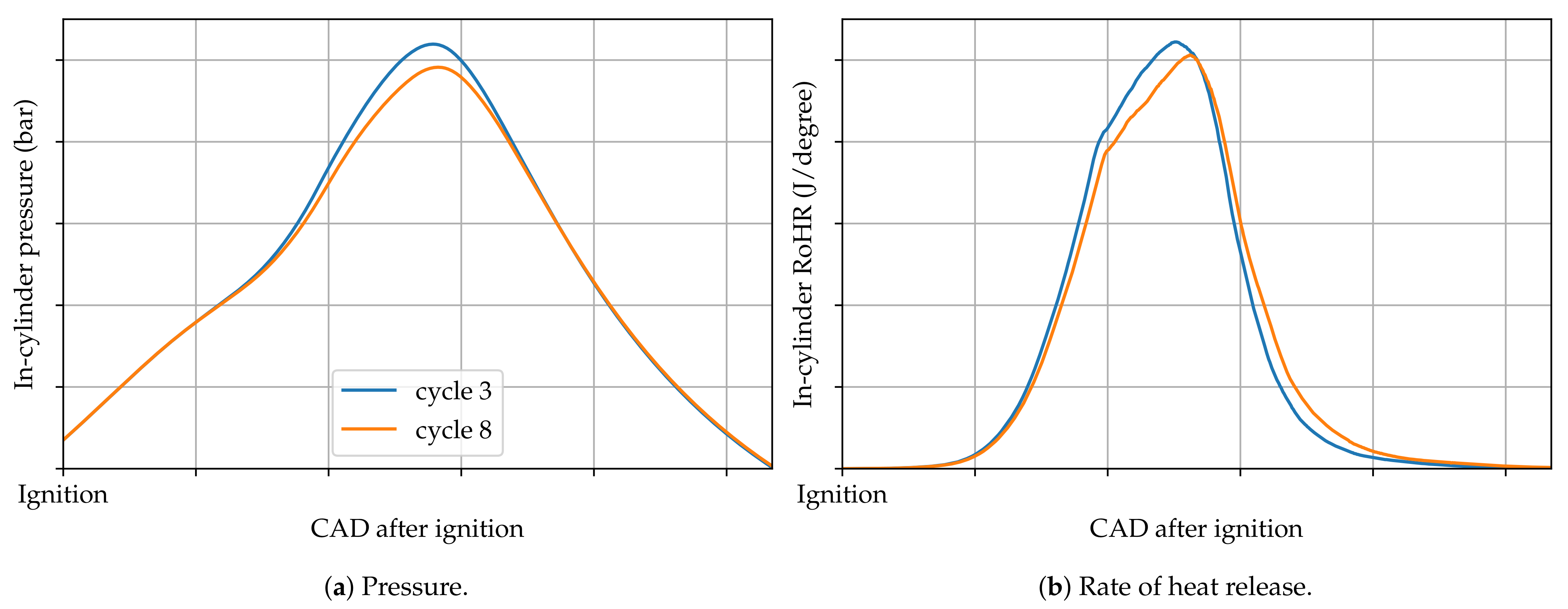
In total, simulations for 16 different combinations are performed and are summarized in Table 1. For the purpose of this work not all cycles are combined with all other cycles. Instead, the two extreme cycles with the minimum and maximum peak pressure, cycles 3 and 8, respectively, are selected for restart file combination with the cylinder pressure and rate of heat release shown in Figure 3. Additionally, this paper only considers the velocity and turbulence quantities as exchange datasets.
Table 2 summarizes results for four combustion metrics for 16 simulations using the combinations listed in Table 1. Respectively, these metrics are peak cylinder pressure (), crank angle degree after ignition of peak cylinder pressure (CAD), crank angle degree after ignition for 50% fuel mass fraction burned (MFB50%) and crank angle duration from 10–90% mass fraction burned (MFB10–90%).
Excluding maximum cylinder pressure, the table shows both absolute values and the percentile in the span from minimum to maximum of the observed range. As previously noted, cycle 3 has the highest peak cylinder pressure and is thus scaled to 100% while cycle 8 has the lowest and is scaled to 0%. Due to the inverse relationship between the combustion metrics and peak cylinder pressure, cycle 3 also has the minimum in the span for the remaining metrics and therefore each of these are scaled to 0%. Similarly, since cycle 8 has the lowest maximum cylinder pressure it also has the maximum in the span for the other metrics and therefore each of these are scaled to 100%.
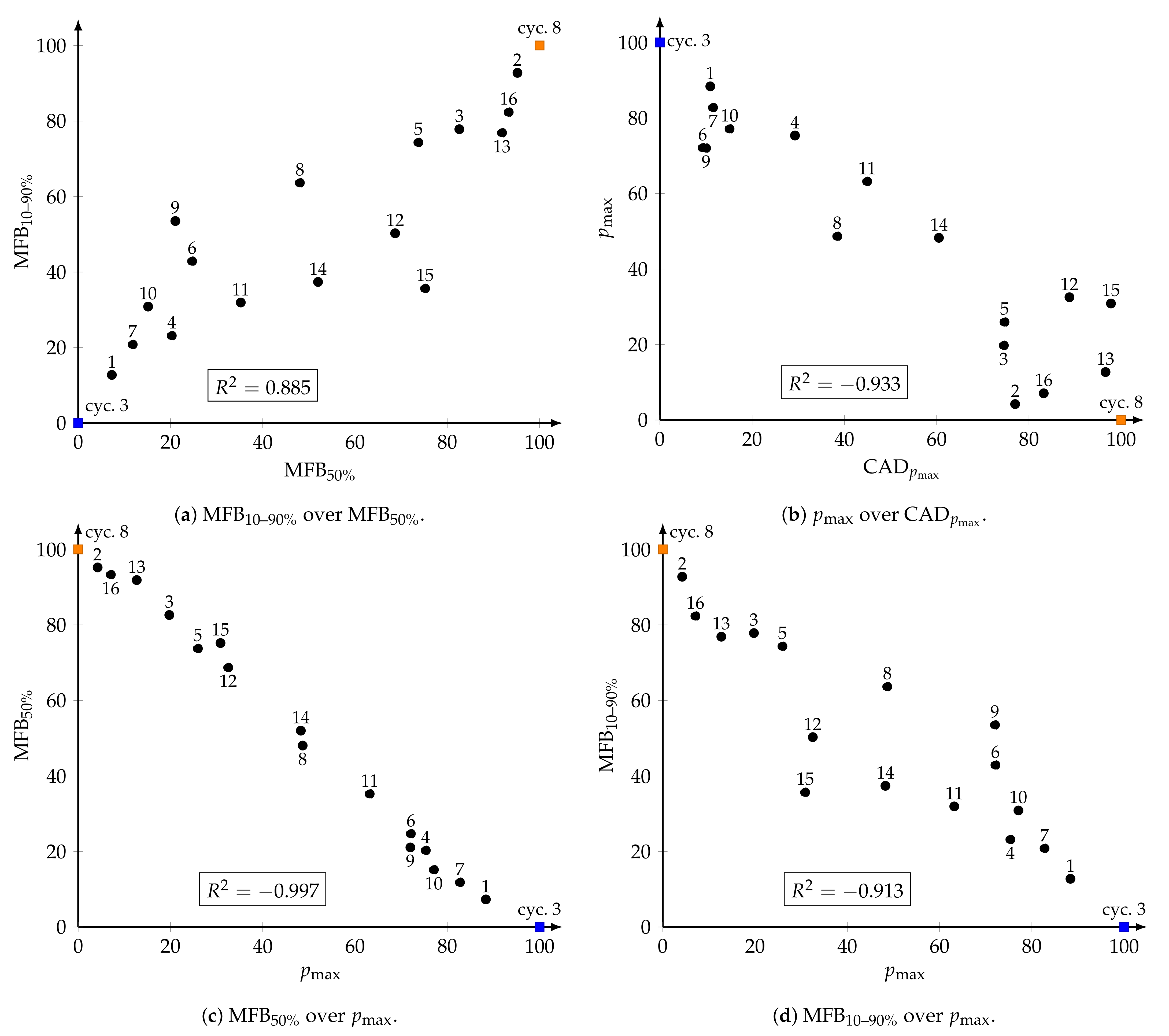
Figure 4 presents the results from Table 2 showing the following: (a) 10–90% mass fraction burned versus 50% mass fraction burn, (b) peak cylinder pressure versus location of peak pressure, (c) 50% mass fraction burned versus peak cylinder pressure and (d) 10–90% mass fraction burned versus peak cylinder pressure. In each figure the results for cycle 3 and 8 are plotted as colored square symbols (blue—cycle 3, orange—cycle 8) and denoted as base. Since cycles 3 and 8 represent either the maximum or minimum observed combustion metric, they fall at the corners within each figure with cycle 3 always at lower left or right and cycle 8 at upper left or right. Results for the 16 simulated combinations are plotted and generally follow a linear relationship between the two base cycle results.
3.1. Impact of the Velocity Field on the Combustion
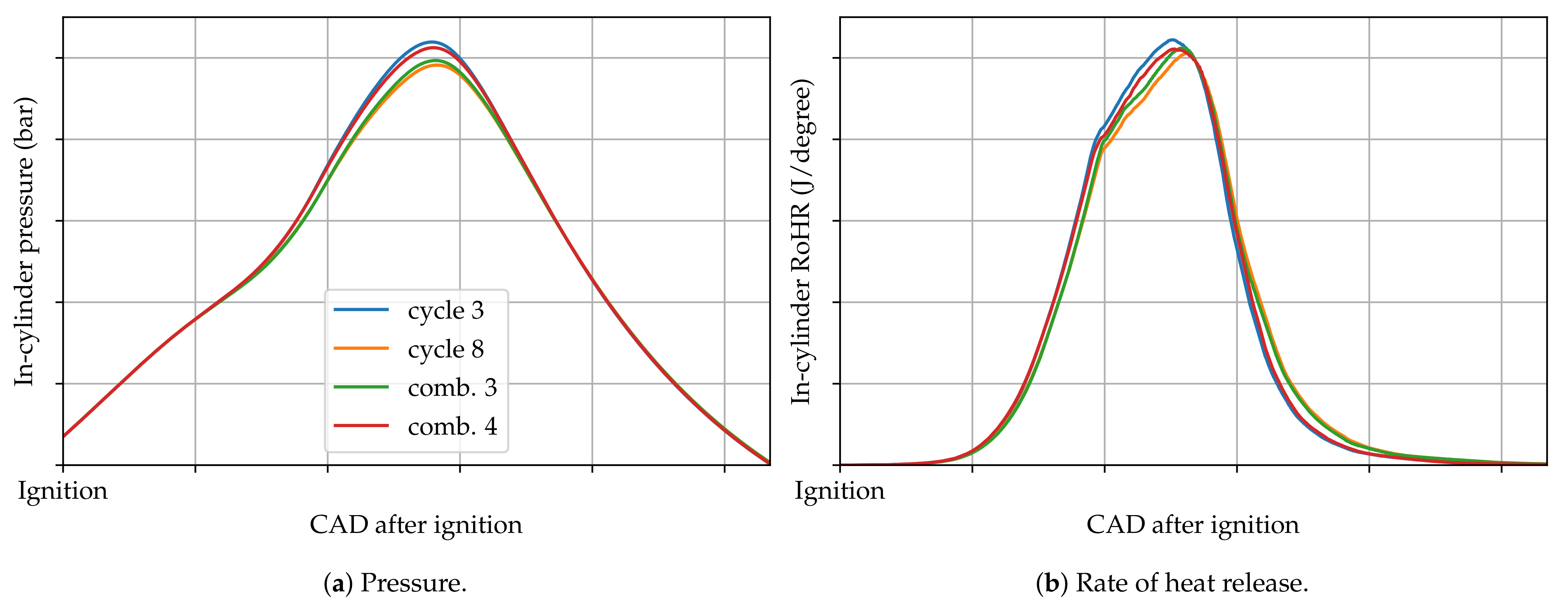
The first two combinations, combination 1 and combination 2, extract the velocity of one of the selected cycles and combine it with all other quantities, excluding the velocity field, from the other cycle. Figure 5 shows the in-cylinder pressure traces and rate of heat releases of the two original cycles and the two combinations. The figure shows in-cylinder pressure is very close to the simulation from which the velocity field is used. The peak cylinder pressure for combination 1 (base of cycle 8) is increased from 0% to 88.3% and decreased for combination 2 (base of cycle 3) from 100% to 4.2%.
Of particular importance are the results for combinations 1 and 2 which exchange only the velocity field of the base cycles while retaining the remaining simulation results. Simply by exchanging the velocity field in the simulation snapshot of cycle 3 with the velocity field of cycle 8 moves the crank angle combustion metrics (CAD, MFB50%) of cycle 3 from 0% (earliest) to the 75 to 90th (late) percentile and close to cycle 8’s metrics. This suggests that the velocity field of cycle 8 plays a significant role in a slowed ignition kernel development and/or turbulent flame propagation.
Similarly, exchanging the velocity field of cycle 3 in the simulation snapshot of cycle 8 moves the crank angle combustion metrics of cycle 8 from 100% (latest) downward to the 5 to 10th (early) percentile suggesting that the velocity field of cycle 3 plays a significant role in an accelerated ignition kernel development and/or turbulent flame propagation. Naturally, this leads to the question of what it is specifically about these two flow fields that appear to drive either a faster or slower combustion regime. This question is out of scope for the present work.
3.2. Impact of the Turbulence on the Combustion
Next, the impact of turbulence, the turbulent kinetic energy k and the rate of dissipation of turbulent energy are investigated. Figure 6 shows the combinations 3 and 4 which exchange only the turbulence field between cycles 3 and 8. The figure shows that the turbulence fields at ignition timing do not play a major role in the combustion event.
However, it is arguable that exchanging the turbulence quantities alone is a proper assessment of the impact of the turbulence on combustion in the context of a two equation uRANS turbulence model, since velocity and turbulence fields have a complex coupling. Figure 7 shows that an immediate relaxation of the turbulence to their prior values does not occur even when the velocity field remains unchanged. Figure 7a shows that the turbulence intensity of combination 1 is much closer to cycle 8 during the ignition phase. This seems plausible since k and are sourced from cycle 8, and only the flow field comes from cycle 3. Similar results and conclusions can be drawn for the other three combinations that are shown in Figure 7b for combinations 2, 3 and 4.
3.3. Impact of the Flow Field near the Spark Plug on the Combustion
Since the first four combinations show that the flow field seems to have the most impact on the combustion, a new combination strategy is considered. For the next combinations, only the flow field in the vicinity of the ignition location (spherical volume with different radii: 1 cm, 2 cm and 5 cm) is extracted and combined with the flow field in the rest of the domain and all other quantities of the other cycle. To assess the impact of changes in the flow field from the initial snapshot to the spark event the time before ignition when the snapshots are taken is varied from 5 CAD to 0.5 CAD.
Combinations 5, 6 and 7 use the flow field in a spherical volume around the ignition location of cycle 3 and all other quantities and the flow field outside of said volume of cycle 8. The in-cylinder pressure and rate of heat release are shown in Figure 8. The time before ignition when the snapshot is taken is 5 CAD. The figure shows that the larger the spherical volume the closer the cylinder pressure is to cycle where the velocity field is sourced with the peak cylinder pressures for combinations 5, 6 and 7 of 25.9%, 72.1% and 82.7% for radii 1 cm, 2 cm and 5 cm, respectively with 100% corresponding to the cycle from which the near spark plug flow field is extracted.
Figure 9 shows the in-cylinder pressure and rate of heat release of combinations 8, 9 and 10, which are similar to combinations 6, 7 and 8, respectively; however, the time of the snapshot is shifted closer to spark timing from 5 CAD to 0.5 CAD before ignition. The impact of this shift is most pronounced on the results using a 1 cm sphere extraction volume. In this case the in-cylinder peak pressure increased from 25.9% to 48.7%. The other two combinations only show a minor change in peak pressure, where combination 9 has almost the same peak pressure as combination 6 (72.0% vs. 72.1%) and combination 10 even shows a significantly lower peak pressure than combination 7 (82.7% vs. 77.1%). This implies that the flow field between the 2 cm and 5 cm spheres only plays a minor role for turbulent flame propagation and that most contributions to CCV are due to the flow field inside the 1 cm sphere.
Combinations 11, 12 and 13, shown in Figure 10, are similar to combinations 5, 6 and 7; only the original cycles are exchanged, i.e., a peak pressure of 0% corresponds to the cycle where the near-ignition flow field comes from. Again, a larger sphere of exchange region means a lower peak pressure, going from 63.2% for the 1 cm sphere to 32.5% for the 2 cm sphere and as low as 12.7% for the largest sphere of 5 cm.
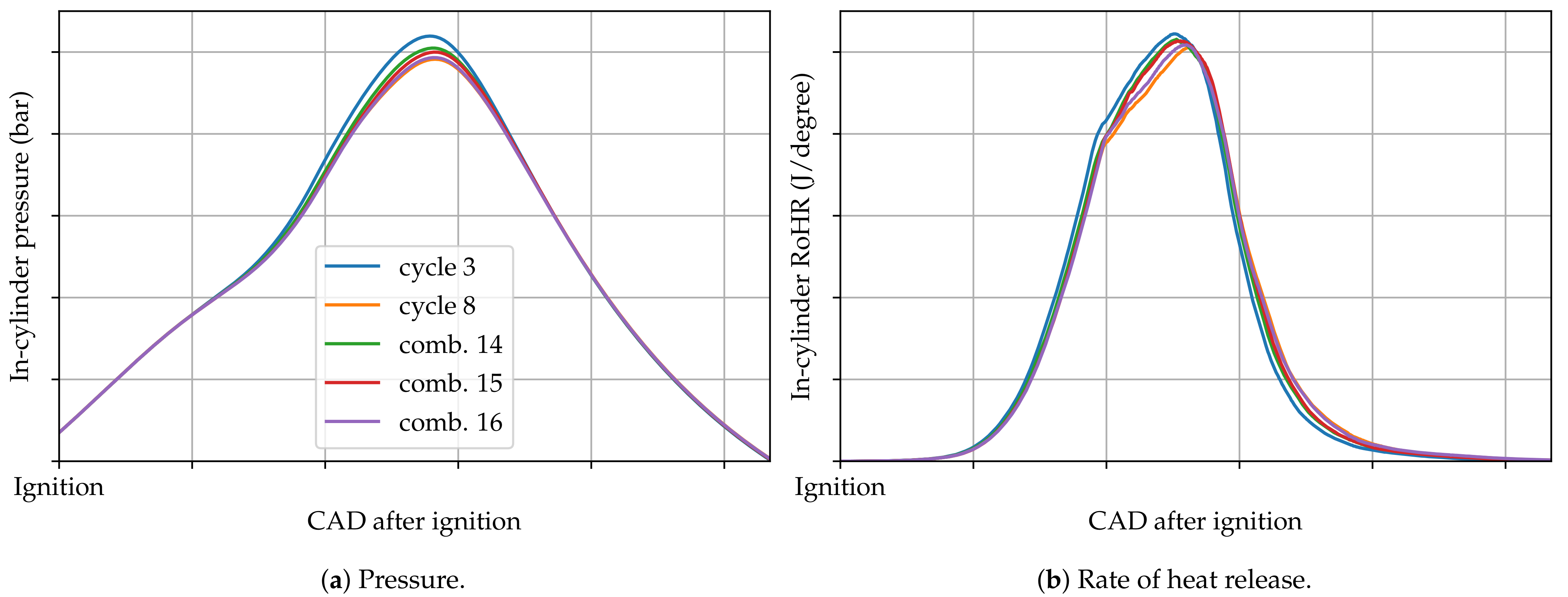
Combinations 14, 15 and 16 are equal to combinations 11, 12 and 13 with the exception of the time when the snapshot is taken being shifted to 0.5 CAD before ignition. This leads to a lower peak pressure, shown in Figure 11, which means that these combinations are closer to the 0% peak pressure cycles than the combinations with an earlier snapshot time.
4. Summary and Conclusions
A novel method for quantifying the individual flow field parameters that impact CCV in the multi-cycle CFD simulation of spark-ignited engines has been presented. The method has been applied to a spark-ignited lean burn natural gas engine and reveals that for this engine and the operating point examined the velocity field has the largest impact on the combustion behavior. Exchanging velocity fields between the slowest/fastest combusting cycles can advance/retard crank angle combustion metrics such as location of peak pressure, 50% mass fraction burned and 10–90% mass fraction burned by 75–90% of the observed span. Applying the methodology to subsets of the physical domain in proximity to the spark plug shows that the velocity field in this region also has a significant impact on the ignition kernel and combustion event.
The methodology indicates that the turbulence field (k and ) for these uRANS simulations plays a significantly minor role as compared to the velocity field. However, it is acknowledged that proper evaluation of the impacts of turbulence may be significantly limited due to the rapid relaxation of the turbulence field when being introduced into a new velocity field, as these systems are not decoupled. As shown in Section 3.2, this relaxation does not take place at least for the average in-cylinder turbulent kinetic energy. Instead, the resulting k field is in between the two extreme cycles.
The cycle-to-cycle variations are rather low (CoV of is 1.15%) in this study and this may be attributed to using the RANS turbulence modeling approach, the same boundary conditions for each engine cycle, same ignition location and/or the same ignition energy for each engine cycle. Regardless, the methodology presented is capable of identifying and quantifying the significance of various drivers for slow and fast combustion events, suggesting it can provide greater insight in instances of much larger CCV.
Author Contributions
Conceptualization, both authors; methodology, C.G.; software, both authors; validation, both authors; investigation, C.G.; resources, C.G.; data curation, C.G.; writing—original draft preparation, both authors; writing—review and editing, S.G.; visualization, C.G. Both authors have read and agreed to the published version of the manuscript.
Funding
Open Access Funding by the Graz University of Technology.
Acknowledgments
C.G. acknowledges the financial support of the “COMET—Competence Centres for Excellent Technologies” Programme of the Austrian Federal Ministry for Climate Action, Environment, Energy, Mobility, Innovation and Technology (BMK) and the Federal Ministry for Digital and Economic Affairs (BMDW) and the Provinces of Styria, Tyrol and Vienna for the COMET Centre (K1) LEC EvoLET. The COMET Programme is managed by the Austrian Research Promotion Agency (FFG).
Conflicts of Interest
The authors declare no conflict of interest. The funders had no role in the design of the study; in the collection, analyses, or interpretation of data; in the writing of the manuscript, or in the decision to publish the results.
Abbreviations
The following abbreviations are used in this manuscript:
| CoV | coefficient of variation |
| CCV | cycle-to-cycle variations |
| CFL | Courant–Friedrichs–Lewy |
| SI | spark-ignited |
| RANS | Renolds-averaged Navier–Stokes equations |
| CFD | computational fluid dynamics |
| AMR | adaptive mesh refinement |
| CAD | crank angle degree |
| MFB | mass fraction burned |
Appendix A
Results from an ordinary restart, i.e., no datasets are exchanged, showing that restarting the simulation has no impact on the combustion behavior.
Figure A1.
In-cylinder results for cycle 3 and restart of cycle 3.

Figure A2.
In-cylinder results for cycle 8 and restart of cycle 8.

References
- Young, M.B. Cyclic Dispersion in the Homogeneous-Charge Spark-Ignition Engine—A Literature Survey. SAE Trans. 1981, 90, 49–73. [Google Scholar] [CrossRef]
- Ozdor, N.; Dulger, M.; Sher, E. Cyclic Variability in Spark Ignition Engines A Literature Survey. SAE Trans. 1994, 103, 1514–1552. [Google Scholar] [CrossRef]
- Maurya, R.K. Combustion Stability Analysis. In Reciprocating Engine Combustion Diagnostics: In-Cylinder Pressure Measurement and Analysis; Springer: Cham, Switzerland, 2019; pp. 361–459. [Google Scholar] [CrossRef]
- Matekunas, F.A. Modes and Measures of Cyclic Combustion Variability. SAE Trans. 1983, 92, 1139–1156. [Google Scholar] [CrossRef]
- Johansson, B. Cycle to Cycle Variations in S.I. Engines—The Effects of Fluid Flow and Gas Composition in the Vicinity of the Spark Plug on Early Combustion. SAE Trans. 1996, 105, 2286–2296. [Google Scholar] [CrossRef] [Green Version]
- Han, S.B. Cycle-to-cycle variations under cylinder-pressure-based combustion analysis in spark ignition engines. KSME Int. J. 2000, 14, 1151–1158. [Google Scholar] [CrossRef]
- Reuss, D.L. Cyclic Variability of Large-Scale Turbulent Structures in Directed and Undirected IC Engine Flows. SAE Trans. 2000, 109, 125–145. [Google Scholar] [CrossRef]
- Abraham, P.S.; Yang, X.; Gupta, S.; Kuo, T.W.; Reuss, D.L.; Sick, V. Flow-pattern switching in a motored spark ignition engine. Int. J. Engine Res. 2015, 16, 323–339. [Google Scholar] [CrossRef] [Green Version]
- Mahmoudzadeh Andwari, A.; Pesyridis, A.; Esfahanian, V.; Said, M.F.M. Combustion and Emission Enhancement of a Spark Ignition Two-Stroke Cycle Engine Utilizing Internal and External Exhaust Gas Recirculation Approach at Low-Load Operation. Energies 2019, 12, 609. [Google Scholar] [CrossRef] [Green Version]
- Marchitto, L.; Tornatore, C.; Teodosio, L. Individual Cylinder Combustion Optimization to Improve Performance and Fuel Consumption of a Small Turbocharged SI Engine. Energies 2020, 13, 5548. [Google Scholar] [CrossRef]
- Omanovic, A.; Zsiga, N.; Soltic, P.; Onder, C. Increased Internal Combustion Engine Efficiency with Optimized Valve Timings in Extended Stroke Operation. Energies 2021, 14, 2750. [Google Scholar] [CrossRef]
- El-Adawy, M.; Heikal, M.R.; Aziz, A.; Rashid, A.; Adam, I.K.; Ismael, M.A.; Babiker, M.E.; Baharom, M.B.; Firmansyah; Abidin, E.Z.Z. On the Application of Proper Orthogonal Decomposition (POD) for In-Cylinder Flow Analysis. Energies 2018, 11, 2261. [Google Scholar] [CrossRef] [Green Version]
- Martinez-Boggio, S.; Merola, S.; Teixeira Lacava, P.; Irimescu, A.; Curto-Risso, P. Effect of Fuel and Air Dilution on Syngas Combustion in an Optical SI Engine. Energies 2019, 12, 1566. [Google Scholar] [CrossRef] [Green Version]
- Schiffmann, P. Root Causes of Cyclic Variability of Early Flame Kernels in Spark Ignited Engines. Ph.D. Thesis, University of Michigan, Ann Arbor, MI, USA, 2016. [Google Scholar]
- Schiffmann, P.; Reuss, D.L.; Sick, V. Empirical investigation of spark-ignited flame-initiation cycle-to-cycle variability in a homogeneous charge reciprocating engine. Int. J. Engine Res. 2018, 19, 491–508. [Google Scholar] [CrossRef]
- Sadeghi, M.; Truffin, K.; Peterson, B.; Böhm, B.; Jay, S. Development and Application of Bivariate 2D-EMD for the Analysis of Instantaneous Flow Structures and Cycle-to-Cycle Variations of In-cylinder Flow. Flow Turbul. Combust. 2021, 106, 231–259. [Google Scholar] [CrossRef]
- Roudnitzky, S.; Druault, P.; Guibert, P. Proper orthogonal decomposition of in-cylinder engine flow into mean component, coherent structures and random Gaussian fluctuations. J. Turbul. 2006, 7, N70. [Google Scholar] [CrossRef]
- Vermorel, O.; Richard, S.; Colin, O.; Angelberger, C.; Benkenida, A.; Veynante, D. Towards the understanding of cyclic variability in a spark ignited engine using multi-cycle LES. Combust. Flame 2009, 156, 1525–1541. [Google Scholar] [CrossRef]
- Liu, K.; Haworth, D.C.; Yang, X.; Gopalakrishnan, V. Large-eddy simulation of motored flow in a two-valve piston engine: POD analysis and cycle-to-cycle variations. Flow Turbul. Combust. 2013, 91, 373–403. [Google Scholar] [CrossRef]
- Li, W.; Li, Y.; Wang, T.; Jia, M.; Che, Z.; Liu, D. Investigation of the effect of the in-cylinder tumble motion on cycle-to-cycle variations in a direct injection spark ignition (DISI) engine using large eddy simulation (LES). Flow Turbul. Combust. 2017, 98, 601–631. [Google Scholar] [CrossRef]
- Richard, S.; Dulbecco, A.; Angelberger, C.; Truffin, K. Invited Review: Development of a one-dimensional computational fluid dynamics modeling approach to predict cycle-to-cycle variability in spark-ignition engines based on physical understanding acquired from large-eddy simulation. Int. J. Engine Res. 2015, 16, 379–402. [Google Scholar] [CrossRef]
- Netzer, C.; Pasternak, M.; Seidel, L.; Ravet, F.; Mauss, F. Computationally efficient prediction of cycle-to-cycle variations in spark-ignition engines. Int. J. Engine Res. 2020, 21, 649–663. [Google Scholar] [CrossRef]
- Truffin, K.; Angelberger, C.; Richard, S.; Pera, C. Using large-eddy simulation and multivariate analysis to understand the sources of combustion cyclic variability in a spark-ignition engine. Combust. Flame 2015, 162, 4371–4390. [Google Scholar] [CrossRef] [Green Version]
- Lauer, T.; Frühhaber, J. Towards a Predictive Simulation of Turbulent Combustion?—An Assessment for Large Internal Combustion Engines. Energies 2021, 14, 43. [Google Scholar] [CrossRef]
- Scarcelli, R.; Richards, K.; Pomraning, E.; Senecal, P.K.; Wallner, T.; Sevik, J. Cycle-to-Cycle Variations in Multi-Cycle Engine RANS Simulations. In Proceedings of the SAE 2016 World Congress and Exhibition. SAE International, Grand Rapids, MI, USA, 7–10 September 2016. [Google Scholar] [CrossRef]
- Krastev, V.K.; Silvestri, L.; Falcucci, G. A Modified Version of the RNG k–ε Turbulence Model for the Scale-Resolving Simulation of Internal Combustion Engines. Energies 2017, 10, 2116. [Google Scholar] [CrossRef] [Green Version]
- Smith, G.P.; Golden, D.M.; Frenklach, M.; Moriarty, N.W.; Eiteneer, B.; Goldenberg, M.; Bowman, C.T.; Hanson, R.K.; Song, S.; William, C.; et al. GRI Mech 3.0. 1999. Available online: http://combustion.berkeley.edu/gri-mech/version30/text30.html (accessed on 26 April 2021).
- Scarcelli, R.; Sevik, J.; Wallner, T.; Richards, K.; Pomraning, E.; Senecal, P.K. Capturing Cyclic Variability in Exhaust Gas Recirculation Dilute Spark-Ignition Combustion Using Multicycle RANS. J. Eng. Gas Turbines Power 2016, 138, 112803. [Google Scholar] [CrossRef]
- Kosmadakis, G.M.; Rakopoulos, C.D. A Fast CFD-Based Methodology for Determining the Cyclic Variability and Its Effects on Performance and Emissions of Spark-Ignition Engines. Energies 2019, 12, 4131. [Google Scholar] [CrossRef] [Green Version]
- Kosmadakis, G.; Rakopoulos, D.; Arroyo, J.; Moreno, F.; Muñoz, M.; Rakopoulos, C. CFD-based method with an improved ignition model for estimating cyclic variability in a spark-ignition engine fueled with methane. Energy Convers. Manag. 2018, 174, 769–778. [Google Scholar] [CrossRef]
- h5py Developers. HDF5 for Python. 2021. Available online: https://www.h5py.org/ (accessed on 28 April 2021).
Figure 1.
One possible combination of restart files: Here, the flow field is extracted from the third cycle and combined with all other quantities of the fifth cycle. The simulation then starts at the time when the fifth snapshot was taken.
Figure 1.
One possible combination of restart files: Here, the flow field is extracted from the third cycle and combined with all other quantities of the fifth cycle. The simulation then starts at the time when the fifth snapshot was taken.

Figure 2.
In-cylinder results for all ten cycles.

Figure 3.
In-cylinder results for the two cycles with the lowest and highest pressure.

Figure 4.
Visualization of combustion charactersitics. All values are relative to the two extreme cycles. The numbers above or below the markers correspond to the combination number.
Figure 4.
Visualization of combustion charactersitics. All values are relative to the two extreme cycles. The numbers above or below the markers correspond to the combination number.

Figure 5.
In-cylinder results for combinations 1 and 2.

Figure 6.
In-cylinder results for combinations 3 and 4.

Figure 7.
Average in-cylinder turbulent kinetic energy.

Figure 8.
In-cylinder results for combinations 5, 6 and 7.

Figure 9.
In-cylinder results for combinations 8, 9 and 10.

Figure 10.
In-cylinder results for combinations 11, 12 and 13.

Figure 11.
In-cylinder results for combinations 14, 15 and 16.


Table 1.
Overview of the different restart combinations.
| Comb. | Base | Exchange | Snapshot Time | Exchanged Datasets |
|---|---|---|---|---|
| 1 | 8 | 3 | 5.0 CAD b. ign. | velocity |
| 2 | 3 | 8 | 5.0 CAD b. ign. | velocity |
| 3 | 8 | 3 | 5.0 CAD b. ign. | turbulence (k and ) |
| 4 | 3 | 8 | 5.0 CAD b. ign. | turbulence (k and ) |
| 5 | 8 | 3 | 5.0 CAD b. ign. | velocity close to spark plug (1 cm sphere) |
| 6 | 8 | 3 | 5.0 CAD b. ign. | velocity close to spark plug (2 cm sphere) |
| 7 | 8 | 3 | 5.0 CAD b. ign. | velocity close to spark plug (5 cm sphere) |
| 8 | 8 | 3 | 0.5 CAD b. ign. | velocity close to spark plug (1 cm sphere) |
| 9 | 8 | 3 | 0.5 CAD b. ign. | velocity close to spark plug (2 cm sphere) |
| 10 | 8 | 3 | 0.5 CAD b. ign. | velocity close to spark plug (5 cm sphere) |
| 11 | 3 | 8 | 5.0 CAD b. ign. | velocity close to spark plug (1 cm sphere) |
| 12 | 3 | 8 | 5.0 CAD b. ign. | velocity close to spark plug (2 cm sphere) |
| 13 | 3 | 8 | 5.0 CAD b. ign. | velocity close to spark plug (5 cm sphere) |
| 14 | 3 | 8 | 0.5 CAD b. ign. | velocity close to spark plug (1 cm sphere) |
| 15 | 3 | 8 | 0.5 CAD b. ign. | velocity close to spark plug (2 cm sphere) |
| 16 | 3 | 8 | 0.5 CAD b. ign. | velocity close to spark plug (5 cm sphere) |
Table 2.
Normalized maximum pressure, CAD after ignition of its occurrence, CAD after ignition of the mass fraction burnt 50% and combustion duration (MFB10–90%).
Table 2.
Normalized maximum pressure, CAD after ignition of its occurrence, CAD after ignition of the mass fraction burnt 50% and combustion duration (MFB10–90%).
| Case | CAD | MFB50% | MFB10–90% | ||||
|---|---|---|---|---|---|---|---|
| Cycle 3 | 100.0% | 36.51 | 0.0% | 31.30 | 0.0% | 17.96 | 0.0% |
| Cycle 8 | 0.0% | 37.03 | 100.0% | 32.20 | 100.0% | 19.21 | 100.0% |
| Comb. 1 | 88.3% | 36.57 | 10.9% | 31.36 | 7.3% | 18.11 | 12.8% |
| Comb. 2 | 4.2% | 36.91 | 77.0% | 32.15 | 95.2% | 19.12 | 92.8% |
| Comb. 3 | 19.8% | 36.90 | 74.6% | 32.04 | 82.6% | 18.93 | 77.8% |
| Comb. 4 | 75.3% | 36.66 | 29.3% | 31.48 | 20.3% | 18.24 | 23.2% |
| Comb. 5 | 25.9% | 36.90 | 74.7% | 31.96 | 73.7% | 18.88 | 74.3% |
| Comb. 6 | 72.1% | 36.56 | 9.3% | 31.52 | 24.7% | 18.49 | 42.9% |
| Comb. 7 | 82.7% | 36.57 | 11.5% | 31.40 | 11.8% | 18.22 | 20.8% |
| Comb. 8 | 48.7% | 36.71 | 38.5% | 31.73 | 48.0% | 18.75 | 63.6% |
| Comb. 9 | 72.0% | 36.56 | 10.0% | 31.49 | 21.1% | 18.62 | 53.5% |
| Comb. 10 | 77.1% | 36.59 | 15.1% | 31.43 | 15.2% | 18.34 | 30.9% |
| Comb. 11 | 63.2% | 36.74 | 44.9% | 31.61 | 35.2% | 18.35 | 31.9% |
| Comb. 12 | 32.5% | 36.97 | 88.8% | 31.92 | 68.7% | 18.58 | 50.3% |
| Comb. 13 | 12.7% | 37.01 | 96.6% | 32.12 | 91.9% | 18.92 | 76.9% |
| Comb. 14 | 48.3% | 36.82 | 60.5% | 31.76 | 52.0% | 18.42 | 37.4% |
| Comb. 15 | 30.9% | 37.02 | 97.8% | 31.97 | 75.2% | 18.40 | 35.7% |
| Comb. 16 | 7.1% | 36.94 | 83.2% | 32.14 | 93.3% | 18.98 | 82.3% |
Publisher’s Note: MDPI stays neutral with regard to jurisdictional claims in published maps and institutional affiliations. |
© 2021 by the authors. Licensee MDPI, Basel, Switzerland. This article is an open access article distributed under the terms and conditions of the Creative Commons Attribution (CC BY) license (https://creativecommons.org/licenses/by/4.0/).
Share and Cite
MDPI and ACS Style
Gößnitzer, C.; Givler, S. A New Method to Determine the Impact of Individual Field Quantities on Cycle-to-Cycle Variations in a Spark-Ignited Gas Engine. Energies 2021, 14, 4136. https://0-doi-org.brum.beds.ac.uk/10.3390/en14144136
AMA Style
Gößnitzer C, Givler S. A New Method to Determine the Impact of Individual Field Quantities on Cycle-to-Cycle Variations in a Spark-Ignited Gas Engine. Energies. 2021; 14(14):4136. https://0-doi-org.brum.beds.ac.uk/10.3390/en14144136
Chicago/Turabian StyleGößnitzer, Clemens, and Shawn Givler. 2021. "A New Method to Determine the Impact of Individual Field Quantities on Cycle-to-Cycle Variations in a Spark-Ignited Gas Engine" Energies 14, no. 14: 4136. https://0-doi-org.brum.beds.ac.uk/10.3390/en14144136
Note that from the first issue of 2016, this journal uses article numbers instead of page numbers. See further details here.