
The Use of Deep Learning Methods in Diagnosing Rotating Machines Operating in Variable Conditions


1
Department of Mechanics and Vibroacoustics, Faculty of Mechanical Engineering and Robotics, AGH University of Science and Technology, al. A. Mickiewicza 30, 30-059 Kraków, Poland
2
Department of Quantitative Methods in Management, Faculty of Management, Lublin University of Technology, ul. Nadbystrzycka 38 D, 20-618 Lublin, Poland
*
Author to whom correspondence should be addressed.
Energies 2021, 14(14), 4231; https://0-doi-org.brum.beds.ac.uk/10.3390/en14144231
Submission received: 20 June 2021
/
Revised: 5 July 2021
/
Accepted: 9 July 2021
/
Published: 13 July 2021
(This article belongs to the Special Issue Smart Energy and Intelligent Transportation Systems)
Abstract
:This paper presents the use of artificial neural networks in diagnosing the technical condition of drive systems operating under variable conditions. The effects of temperature and load variations on the values of diagnostic parameters were considered. An experiment was conducted on a testing rig where a variable load was introduced corresponding to the load of the main gearbox of the bucket wheel excavator. The signals of vibration acceleration on the gearbox body, rotational speed, and current consumption of the drive motor for different values of oil temperature were measured. Synchronous analysis was performed, and the values of order amplitudes and the corresponding values of current, speed, and temperature were determined. Such datasets were the learning vectors for a set of artificial deep learning neural networks. A new approach proposed in this paper is to train the network using a learning set consisting only of data from the efficient system. The responses of the trained neural networks to new data from the undamaged system were performed against the response to data recorded for three damage states: misalignment, unbalance, and simultaneous misalignment and unbalance. As a result, a diagnostic parameter as a normalized measure of the deviation of the network results was developed for the faulted system from the result for the undamaged condition.
1. Introduction
Monitoring systems using vibration signals are often used in the industry to diagnose the technical condition of machinery. Systems based on parameters such as RMS (root mean square), crest factor, and peak of vibration signal are perfect for machines operating in constant operating conditions, where one can assume threshold values for these parameters, whereby exceeding them signals a system fault. However, these parameters are not sufficient to diagnose machines operating under variable loads caused by varying operating conditions [1]. Variable loading causes a change in speed, which makes diagnosis difficult using classical methods based on spectral analysis of the time signal. Synchronous methods are used in the diagnosis of machines operating at variable speed, which are based on the synchronization of the signal carrying diagnostic information with the rotational speed of the tested object [2,3,4,5]. However, varying operating conditions such as load or operating temperature can also affect the amplitude of the diagnostic signal [6,7,8,9,10]. An increase in amplitude due to a variable load can be misinterpreted by monitoring systems. Therefore, this impact must be considered in the monitoring process. A previous study [1] investigated the effect of load and speed on the amplitude values of the characteristic components and proposed a method for scaling these parameters. It is also possible to find papers on diagnosing a planetary gearbox operating under variable conditions, which addressed the problem of changing parameter values from load [7,11]. The solution to this problem can be realized using artificial neural networks [12,13,14,15]. The authors of [16] presented a one-dimensional multi-scale domain adaptive network in bearing diagnostics for different degrees of load. The preliminary preparation of diagnostic signals is important in using neural networks to diagnose machines working in variable conditions. In [17], higher-order spectral analysis and multitask learning were used. However, in [18], a method of learning a convolutional network was proposed using a labeled date and pseudo-labeled date. The measurement of drive motor current in diagnosing gear damage and bearings [19,20,21] is increasingly being used. The presented cases used artificial neural networks as classifiers. In the learning process, vectors for the undamaged and damage states were used as inputs of the network. However, in industrial conditions, especially in the heavy industry, there are no measurement data registered during damage because not all machines are monitored, and the drive system components are produced in small amounts. Moreover, it is impossible to predict all types of faults and introduce them into the network learning process. Accordingly, we propose a solution based on learning neural networks with data recorded only during fault-free operation, which analyzes the responses of the trained networks to signals recorded when faults are introduced.
This paper presents the use of artificial neural networks in diagnosing the technical condition of drive systems operating under variable conditions. The effects of temperature and load variations on the values of diagnostic parameters were considered. An experiment was conducted on a testing rig, where a variable load was introduced, corresponding to the load of the main gearbox of the bucket wheel excavator. The vibration acceleration, speed, and current signals feeding the drive motor were recorded for different values of oil temperature. Synchronous analysis was performed, and the values of order amplitudes and the corresponding values of current, speed, and temperature were determined. Such datasets were the learning vectors for a set of artificial neural networks.
This article presents a new approach to diagnosing machines working in variable conditions. Instead of analyzing the order spectrum, an analysis of the amplitudes of orders as a function of changes in speed, current, and temperature was carried out. A new approach proposed in this paper is to train the network using a learning set consisting only of data from the efficient system. In the next step, the behavior of such a trained neural network on new data from the undamaged system was investigated in comparison with the response to data recorded during three fault conditions of the drive system. As a result, a diagnostic parameter as a normalized measure of the deviation of the network results was developed for the faulted system from the results for the fault-free condition.
2. Materials and Methods
2.1. Testing Facility Description
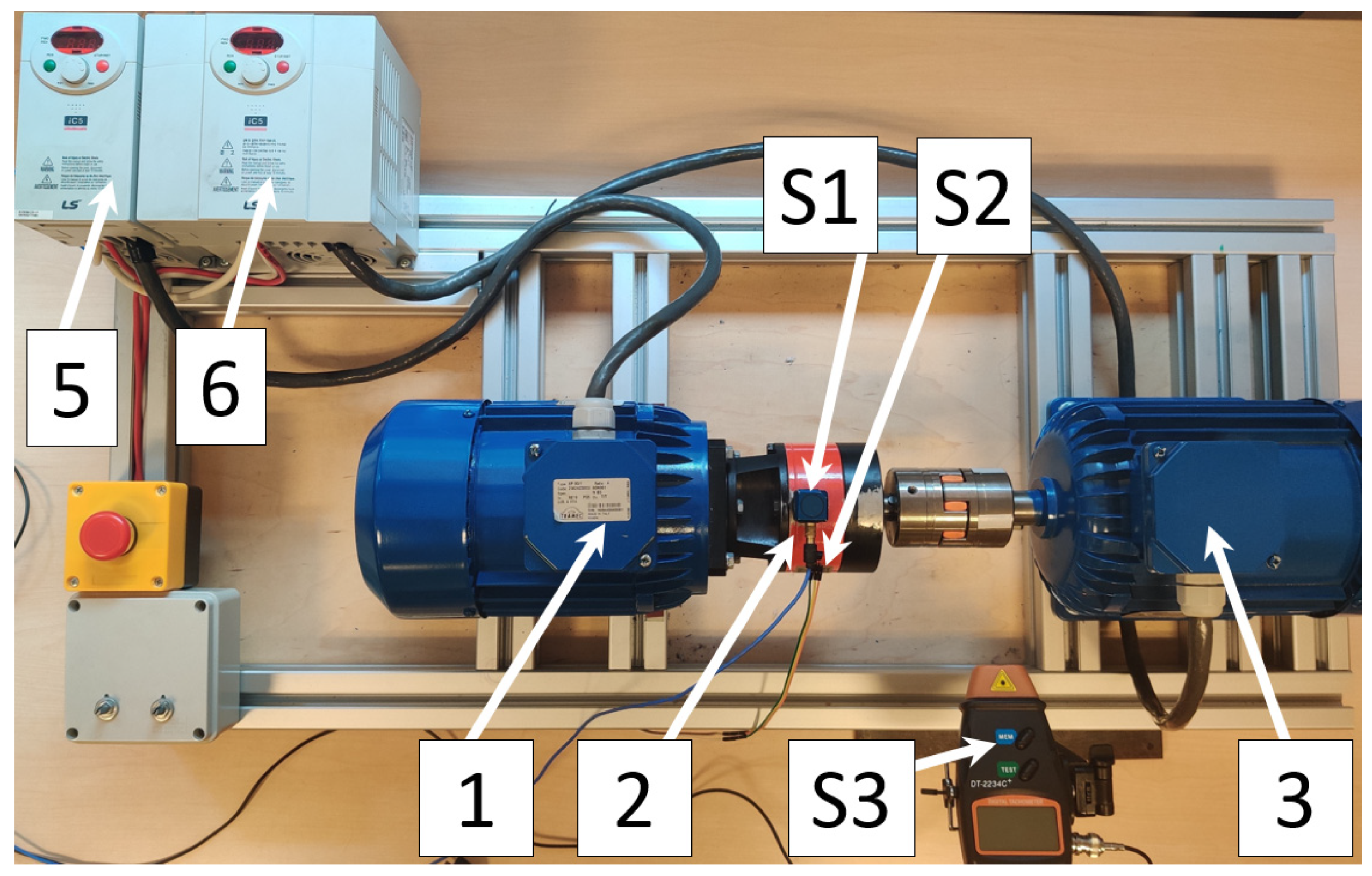
The testing rig (Figure 1) consisted of a TRAMEC EP 90/1 planetary gearbox driven by an electric motor controlled by a frequency converter. The load consisted of a second induction motor connected to the gearbox by a jaw coupling. The load motor was also controlled by a frequency converter, which allowed setting any load function of the system.
Vibration acceleration on the planetary gear case was measured using a PCB 356B08 triaxial acceleration sensor, the temperature was measured using an LM35 sensor, speed was measured using a laser tachometer, and electrical current was measured using an ACS714 sensor. All measurements of the experiment were obtained using a specially built measuring system based on the PXI platform (PCI Extension for Instrumentation). The platform comprised the PXI Trigger Bus, which allows measurement synchronization between individual measuring cards.
2.2. Diagnostic Experiment
Measurements were made for four drive system conditions, which are shown in Table 1.
The misalignment condition (F1) consisted of placing 0.5 mm thick shims under the front feet of the drive motor. The unbalance condition (F2) was introduced by placing additional mass (13 g) on the output shaft coupling. Condition F3 consisted of the simultaneous introduction of misalignment and unbalance. Signals of 30 min duration were recorded for each condition. Measurements were carried out when warming up a system for a temperature in the range of 35–40 °C.
The variable load changes from 1.3 Nm to 4.0 Nm were entered into the system. This caused a change in the rotational output shaft speed of 730–758 RPM and in the RMS value of drive motor current in the range of 2.48–2.51 A. The system was subjected to a variable load corresponding to the load occurring on the main gear of the bucket wheel excavator. The reference signal was obtained from the KWK 1500 s excavator main gear monitoring system, the subject of the patent in [22]. The main gear of the bucket wheel excavator is a bevel-planetary gearbox that drives a bucket wheel. The input of the bucket in the ground causes the system load. With a fixed set voltage value on the drive engine, the load causes a change in speed and vibration amplitude. Diagnosing the main gear of the wheel excavator has already been addressed in [7,11,23], which investigated the signals coming from industrial conditions. However, in industrial conditions, a controlled experiment with given damage cannot be carried out. Therefore, the experiment was carried out in laboratory conditions. The variable load-induced velocity change signals recorded under industrial conditions were scaled up to the capabilities of the laboratory bench.
2.3. The Method of Determining Diagnostic Parameters
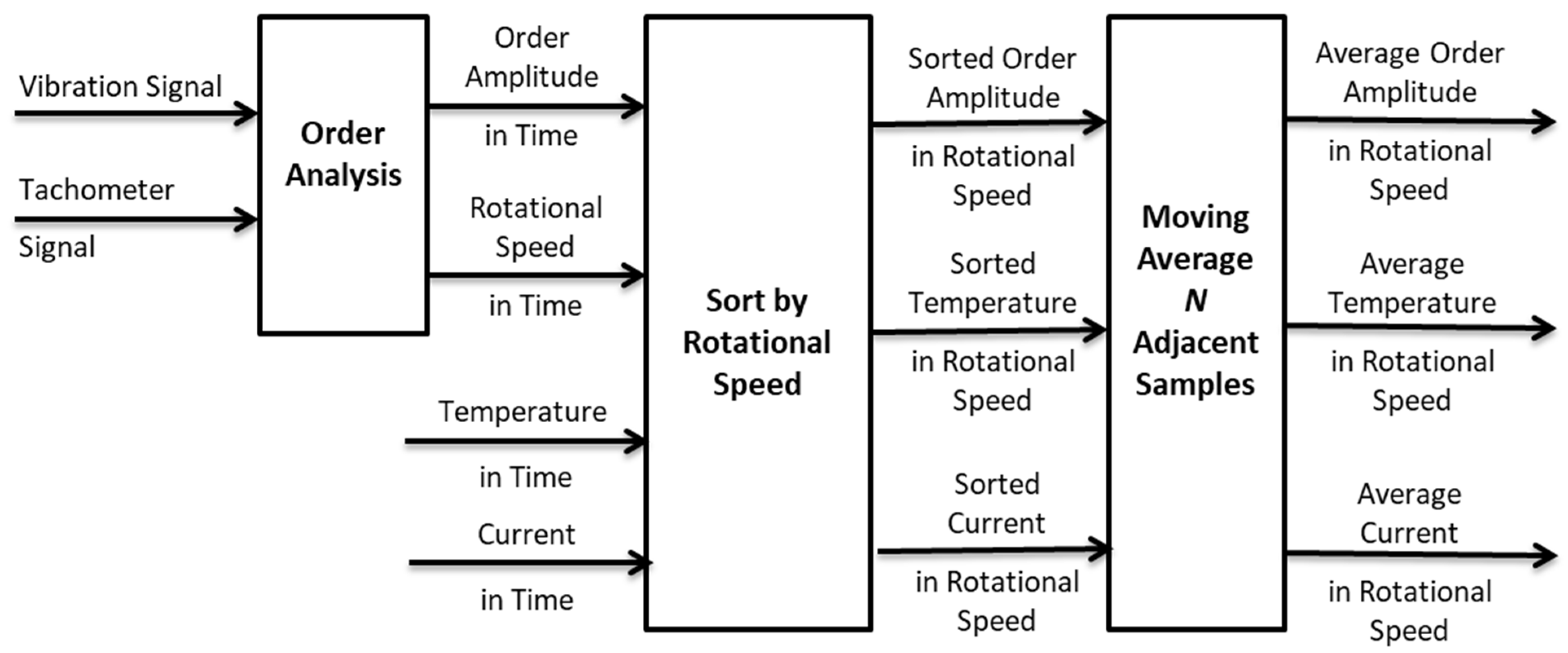
The proposed signal analysis method is based on the order analysis algorithm. The order spectrum is determined using a method based on resampling the vibration acceleration signal against the input shaft speed. Figure 2 shows the schematic of the order analysis algorithm. In the first phase, the tachometer signal is subjected to an interpolation procedure using a cascaded integrator–comb filter (CIC). Next, on the basis of filtered tachometer signal, a vibration signal resampling procedure is performed to determine the vibration signal against the rotation angle (even angle signal). In the resampling method, time samples are converted to angle samples. The time samples are samples of the physical signal that are equally spaced in time. The angle samples are samples that are equally spaced in the rotation angle. The signal resampled as such can be subjected to a fast Fourier transform (FFT), the result of which is an order spectrum. An order spectrum represents amplitude as a function of order rather than as a function of frequency. The orders correspond to multiples of the rotational frequency of the shaft on which the speed measurement is performed [24]. In the case under consideration, the rotational speed measurement is carried out at the output shaft of the gearbox.
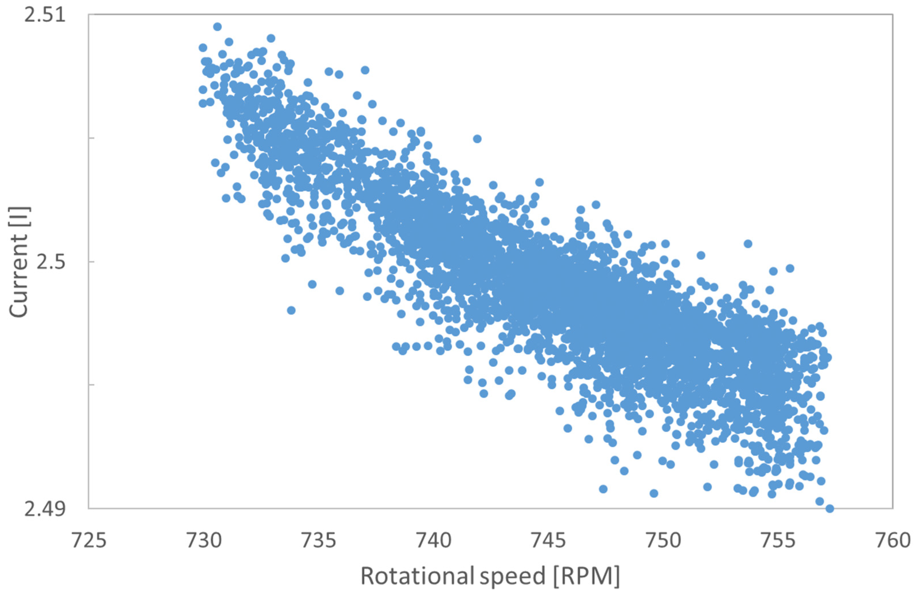
In addition to the averaged order spectrum, the time course of the amplitudes of the individual orders can be obtained from the order analysis. Information about the technical condition of the tested object can be obtained by monitoring the amplitudes of the characteristic orders. However, the change in amplitudes can also be caused by a change in the load on the system [6,25]. The load can be measured indirectly by measuring the electrical current consumption of the drive system. However, it is not always possible to accurately measure electrical current in industrial conditions, especially a measurement synchronized with a vibration measurement. However, in industrial settings, the driving motor is often supplied with a constant voltage and frequency, and any variation in speed is due to a change in load. The relationship between load change and speed recorded on the testing rig is shown in Figure 3. The rotational speed decreased as a result of the increase in the system load, while the load increase resulted in a higher power consumption by the driving motor.
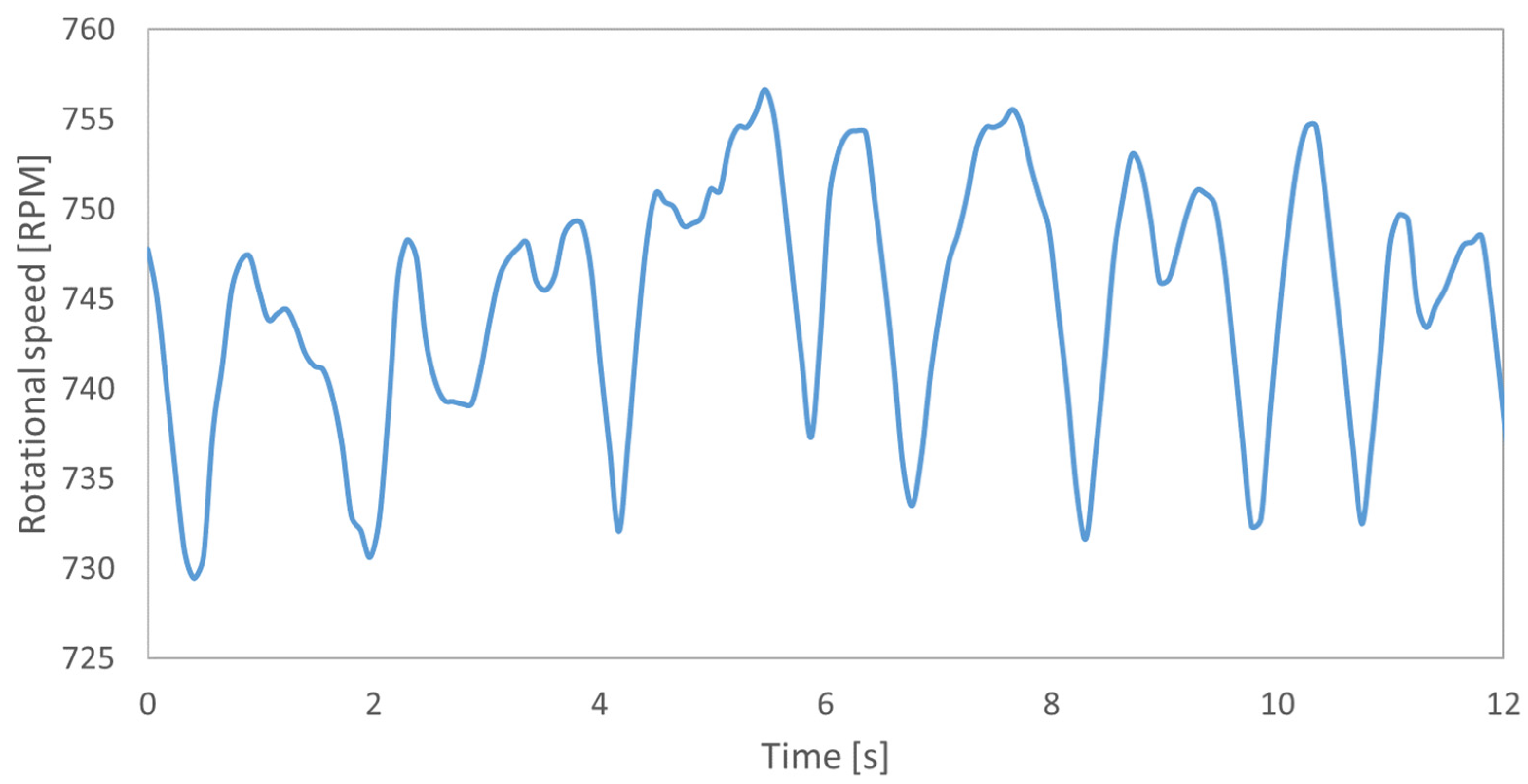
In the test object, the rotational speed was determined by measuring the keyphasor signal. This measurement was synchronized with the vibration acceleration measurement, allowing load variations to be included in diagnostic estimates, such as characteristic component amplitudes. Figure 4 shows the speed waveform of the input shaft of the diagnosed object during operation under load. Speed changes were caused by changes in the system load because the frequency and voltage applied to the motor driving the system were constant. A similar case can be encountered in industrial settings. In the experiment conducted, rotational speed variation waveforms recorded on the main gear drive system of a bucket wheel excavator were used. The shape of the rotational speed variation waveform shown in Figure 4 corresponds to the waveform recorded on the main gear of a wheeled excavator operating in a brown coal mine.
Changes in rotational speed associated with varying load resulted in a significant change in the amplitude of the characteristic orders. The value of the order amplitude for the loaded and unloaded system changed significantly, hindering the diagnosis based on this parameter. Figure 5 shows the meshing order amplitude (no. 72) as a function of rotational speed for the efficient system, which varied under load. For maximum rotational speed value, a small load was applied to the system. As the load increased, the speed decreased, while the value of the meshing order amplitude increased because of the interaction between the teeth increasing.
The values of ordinate amplitudes are also affected by temperature, and this was shown in [9]. Diagnostics should be performed for a constant temperature or by considering its influence during inference. Therefore, temperature waveforms measured on the gearbox body were also recorded.
Changes in amplitudes of characteristic orders in the order spectrum are usually analyzed in vibroacoustic diagnostics. According to the literature [6,26,27,28], individual faults or installation defects are characterized by changes in the amplitudes of the corresponding orders, e.g., a change in the amplitude of order no. 1 is symptomatic of unbalance, while a change in the order corresponding to the number of claws of the jaw coupling is due to system misalignment. Therefore, each order obtained from the order spectrum was considered separately because the characteristics of the order amplitudes as a function of load (rotational speed) would change with failure for each order in a different way [25].
As a result of the order analysis, 100 consecutive orders of vibration acceleration recorded in the direction parallel and perpendicular to the shaft axis were obtained. Current, temperature, and speed were recorded simultaneously. Signals of 30 min duration were recorded for each condition. Next, all the recorded signals were divided into time frames of 30 s each. Sets of signals of this length were sequentially subjected to the processing algorithm shown in Figure 6. The processing time of 30 s signals was shorter than 30 s; therefore, the algorithm can be implemented in continuous monitoring systems.
This procedure was performed for data recorded during correct operation (F0) and for signals recorded for individual faults F1, F2, and F3.
First, the vibration signal was subjected to order analysis. The results of this analysis were the waveforms of order amplitudes and speed over time. Figure 6 shows the case for one order. The waveforms of order amplitude, speed, temperature, and current were then sorted in ascending order with respect to speed. The results of such sorting were the courses of these parameters relative to the rotation speed. The next step was to determine the moving average for consecutive elements. Averaging was used to reduce data scatter. The data thus prepared were input vectors for artificial neural networks.
2.4. Using the Artificial Neural Network for Condition Assessment
Deep learning artificial neural networks were used to evaluate the condition of the diagnosed drive train. The idea behind the method was to design the learning process of the neural network such that it detects abnormal situations in systems where faults have not historically occurred or have occurred so infrequently that typical classifiers based on supervised learning could not be used. Accordingly, only data from the undamaged system were used for the learning process.
In addition, it was considered that neural network learning is more efficient when there are significantly fewer outputs than the input data variables [29,30,31]. For this reason, instead of one model evaluating all 100 orders simultaneously, a separate model was built for each order.
From a diagnostic perspective, the best solution would be to reduce the diagnostic decision to a single numerical parameter. Therefore, the system was designed to produce a synthetic diagnostic parameter for each order by exploiting the ability of deep neural networks to recognize patterns autonomously [32,33]. Moreover, some theoretical results suggested that network-based systems can lead to proper robustness [34].
The input data vector for each network were , with its components including the following values, in respective order:
- output shaft rotational speed;
- oil temperature;
- the current drawn by the motor;
- amplitude values of order k in the x-axis;
- z-axis amplitude values of the order k;
- a 30-neuron layer with RELU activation function and a drop-out layer with a drop rate of 20%;
- a 20-neuron layer with RELU activation function and a drop-out layer with a drop rate of 10%.
The output layer of the individual networks consisted of a single neuron returning a numerical value, which, for the correct state of the machine (F0), should return values close to the constant value determined in the network learning stage. In the experiment conducted, the conventional value of this constant was taken as
The expected effect of modeling was that the applied neural network should realize some continuous transformation [32] with the property described in Equation (1).
where is the function from R5 in R with the property that is significantly different from 0, is the vector containing data from the undamaged system for order , is the vector containing data from the faulty system (F1, F2, or F3) for order , is the index of the input vector, , and .
This means that, if then the value of the function should be close to the value of . However, if the vector corresponds to the operation of the defective transmission, the neural network should return a value different enough from such that, taking into account the amount of variance, this difference could be detected by statistical analysis. Since the transformation in Equation (1) is continuous, this guarantees the stability of the network (similar values of the network response come from similar input values). There are some papers where similar observations were made for obtaining stabilization of randomized systems [37].
The primary task in constructing such an architecture is to avoid network overfitting. Due to the fact that we only used the data of a well-functioning machine during the network learning process, such a network may tend to adjust the weights in such a way that, regardless of the output, it returns a response equal to the learned value (i.e., returning a parameter close to regardless of the input state). Therefore, the network training process used as input a set of vectors associated with the state F0. On the other hand, random values from the distribution were generated as the output vector. Adding a perturbation with a small variance to the output vector, as early as at the network learning stage, reduced the risk of trivializing the function realized by the neural network.
Further reducing the risks associated with overfitting involved the following steps:
- using drop-out layers in the network architecture and randomizing the network by randomly deactivating neurons during learning;
- the learning set was randomly divided into a learning set and a validation set (which the network did not formally use for learning).
In addition, the use of these operations renders the network training process nondeterministic, such that the process of training the network for each order can be repeated independently, each time obtaining slightly different values of the weights in each layer, for the same input data. One can notice that this feature of the training process can be exploited to implement the bagging technique. The learning process was, therefore, repeated 120 times, resulting in 120 network models for each order. This approach provided a key mechanism to reduce the risk of system overfitting, as it dispersed this risk across multiple, independent models. In order to achieve that dispersion, evaluation values for 120 models were considered instead of considering the evaluation of a single model. The algorithm of the learning process is shown in Figure 7.
2.5. Verification of Artificial Neural Network Functionality
The functionality of the obtained model was verified after the network learning process. The responses of the proposed solution were investigated when the vectors obtained from the measurements for the machine fault conditions F1, F2, and F3 and for the correct operation state F0 were input. Vectors that were not used during network learning were used to verify the undamaged conditions.
The network response values were determined for all orders, . Next, the average value was determined for each order according to the following relationship:
where is the number of input vectors, is the index of the input vector, and is the i-th output value of the network for the k-th order.
This process was then repeated for 120 trained models. The 120 values of the parameter were obtained for each order. This process was repeated for each condition of the tested drive train. The process of analyzing the functionality of the learned neural network for the F1 condition is shown in Figure 8.
For verification, ratings for states with damage were compared to ratings for a defect-free system. Verification of whether the average of 120 evaluations for each order differed significantly from the average of 120 evaluations for condition F0 was conducted using an ANOVA test.
Two independent input datasets of the undamaged system were used when testing the response for the undamaged system. This approach allowed not only determining whether there was a statistically significant difference between the network response to the fault condition and the response to the no-fault condition, but also measuring the magnitude of the observed discrepancy in a normalized way using the parameter . According to the recommendations [38], negative values of this coefficient, which occur when the size of the noise exceeds the size of the effect, were treated as zeros. Taking this correction into account, the value is described by Equation (3).
where is the sum of squares of the effect from the ANOVA test, is the number of degrees of freedom of the effect from the ANOVA test, is the total sum of squares from the ANOVA test, and is the mean squared error of the residuals from the ANOVA test.
The parameter allows a numerical evaluation normalized to the interval [0, 1] of the deviation of the results obtained from the neural networks for a given technical condition from the result for the condition without faults. The values of the parameter can be classified by determining the power of the effect on the Cohen scale [39] (Table 2).
3. Results and Discussion
3.1. Results of the Order Analysis
When analyzing the spectrum of orders of vibration acceleration signals recorded during machine operation at variable load (Figure 9and Figure 11), a significant standard deviation can be observed for the gear coupling band (orders around coupling order no. 72). This scatter is caused by the high dynamics of the load (Figure 4) applied to the planetary gearbox.
Figure 9 shows the spectra of vibration acceleration orders (vertical direction) for the system without damage (black) and with the introduced misalignment (red).
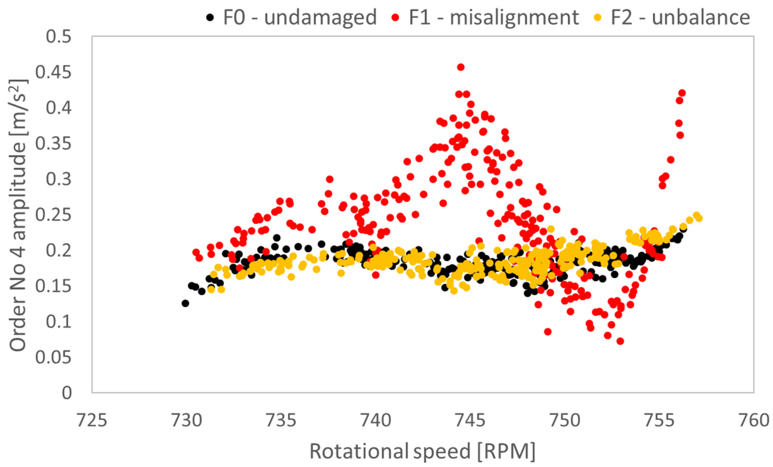
In the case of misalignment, one would expect an increase in the amplitude of order no. 4 corresponding to the number of clutch teeth. However, there is a noticeable increase in amplitude near the coupling band—orders no. 60 to 70. On the other hand, observing the dependence of the amplitude of the order no. 4 as a function of rotational speed (Figure 10), we can observe more than a twofold increase for the speed equal to 745 RPM and for the speed over 755 RPM. Moreover, in the range of 748–755 RPM, the values for the amplitudes for the misaligned system are smaller than those for the efficient system. On the order spectrum, the difference is smaller because the order spectrum represents a value averaged over a period of over a dozen rotations.
Comparing the order spectrum from the undamaged system with the order spectrum from the imbalanced system, it is difficult to see the increase in order no. 1 amplitude, which is symptomatic of this damage (Figure 11). These differences are relatively small when compared to the values of the coupling order amplitudes. However, the order no. 1 has a much smaller standard deviation than the orders in the coupling band of Figure 11.
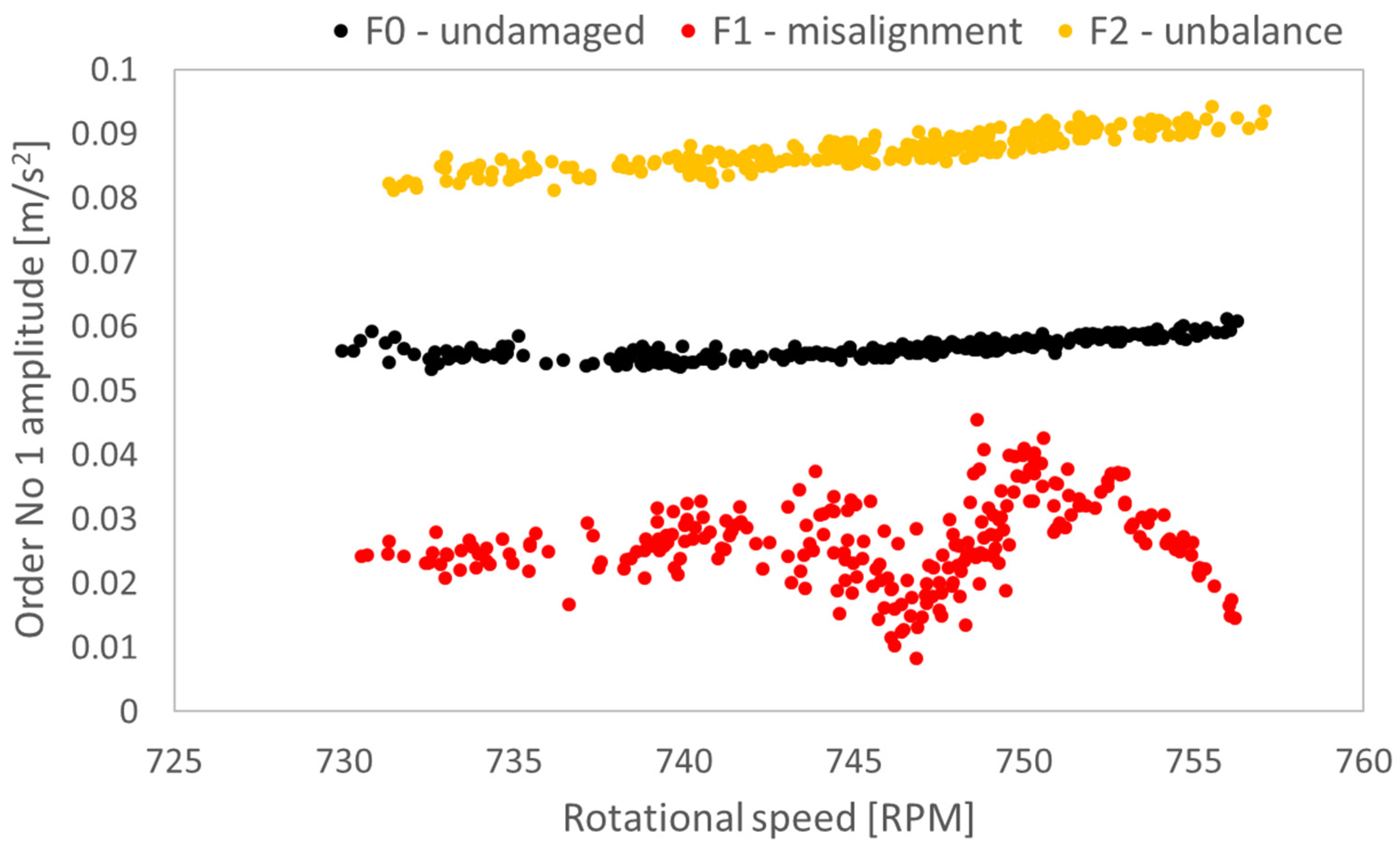
A much smaller scatter of amplitudes of the order no. 1 for unbalance than for misalignment is also seen in Figure 12. However, the amplitude for the alignment signal increased for the entire speed range by a value of 0.04 m/s2, constituting more than 70% of the initial value.
In the case of variable load with a dynamic character causing speed changes shown in Figure 4, the analyzed damage is hardly visible in the order spectrum. Significant changes are visible only after careful analysis of the dependence of the amplitudes of the individual orders on the changes in rotational speed, which are caused by the change in load. Therefore, it is necessary to take into account the changes in ordinate amplitudes due to loading in the diagnosis process.
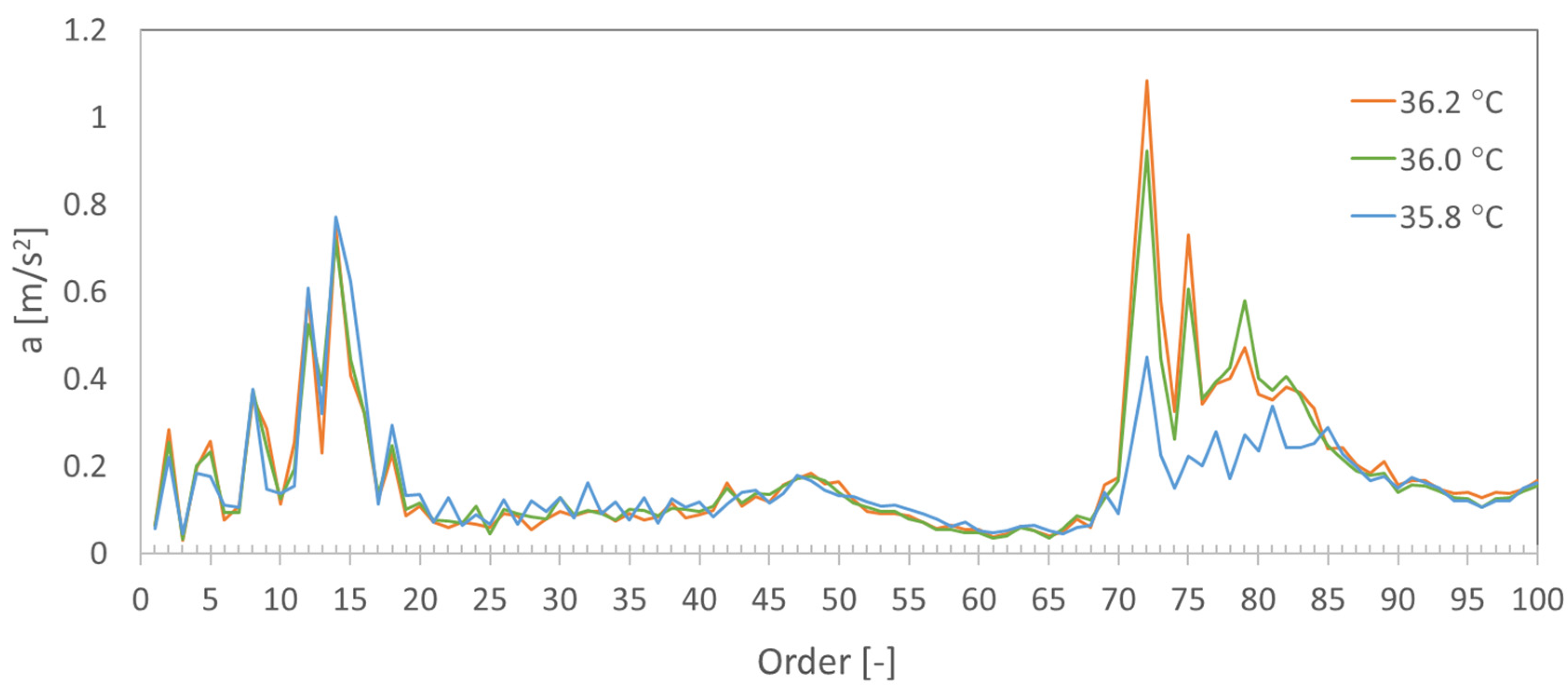
Temperature also has a significant effect on the values of order amplitudes in the interlocking band. Figure 13 shows the order spectra of vibration acceleration for the signal recorded for different temperatures. There is a clear increase in order amplitudes occurring with increasing temperature. This confirms the need to consider the temperature in vibroacoustic diagnostics.
3.2. Results Obtained from Deep Learning Neural Networks
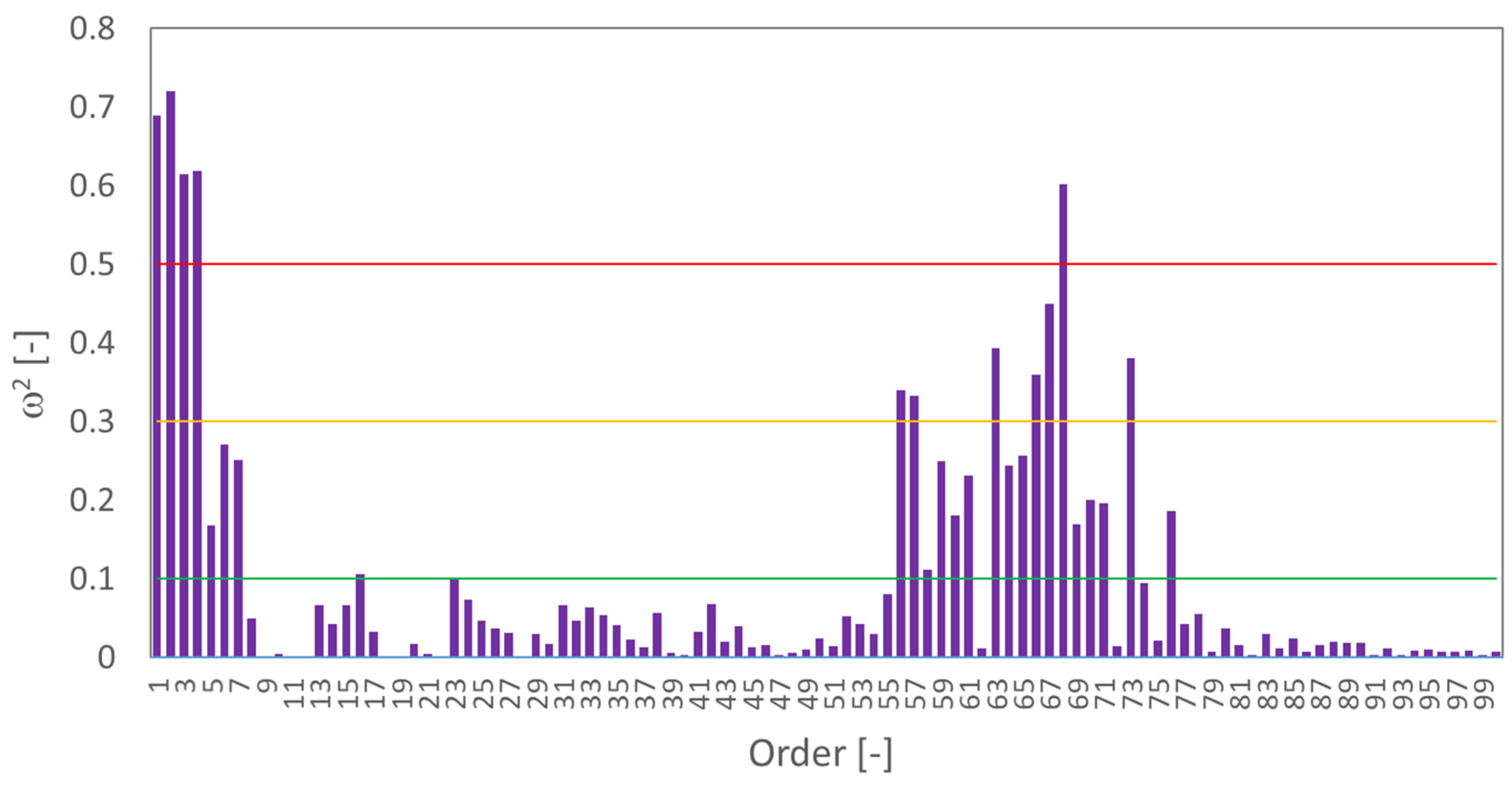
(Figure 14, Figure 15 and Figure 16) show the values of the parameter for each order. This parameter is a numerical evaluation of the deviation of the results obtained from the set of neural networks for a given fault from the results obtained for the no-fault condition.
First, the control data from the measurement for the undamaged system (F0) were provided to the input of the trained networks. These values for all orders were 0, indicating no effect according to the Cohen scale.
Figure 14 shows the values of the parameter for the misalignment condition (F1). A large effect size can be observed for orders no. 1, 2, 3, 4, and 68, while a moderate effect can be observed for orders near the coupling order. The increase in the parameter for order no. 4 is most reasonable and is related to the number of teeth in the coupling used. On the other hand, large values of the parameter for the coupling band may be due to increased inter-tooth interaction during system misalignment.
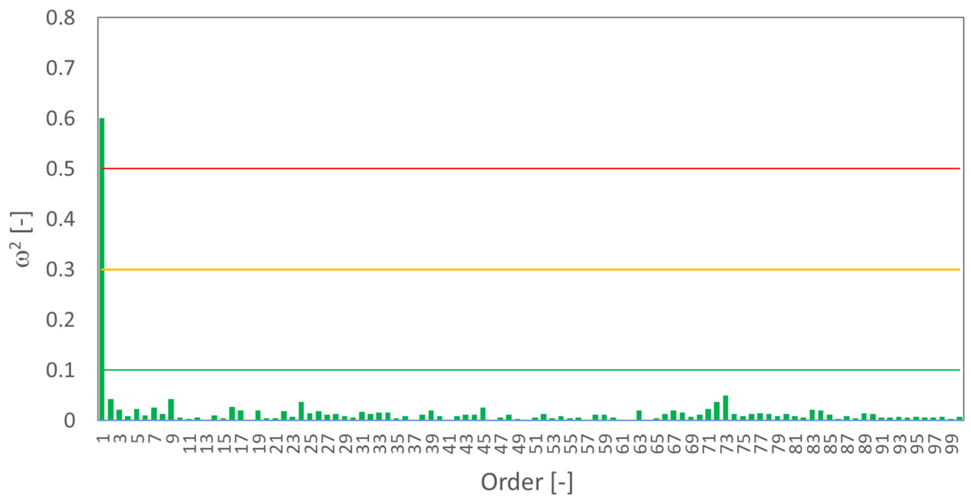
For the unbalanced condition (F2) (Figure 15), a large effect of the Cohen scale is observed only for order no. 1. The values of the parameter for the other orders indicate no effect (differences between the response of the network to the condition F2 and F0). This is consistent with theory because unbalance affects the order no. 1 amplitude values with respect to the shaft on which it occurs.
In the case of the F3 condition (Figure 16), where both faults were introduced, similar values of the parameter can be observed as in the F1 condition. However, the effect of unbalance is also evident by the increased amplitude for the parameter for order no. 1.
4. Conclusions
This paper presents the problem of diagnosing machines operating under variable conditions. A diagnostic experiment was conducted on a testing rig for diagnosing a planetary gearbox. The effects of varying load and oil temperature on vibration acceleration signals measured on the body of a planetary gear that was part of the drive system were analyzed.
For the applied variable load, the use of order spectrum was not sufficient to diagnose the introduced drive train damages. This paper shows that the analysis of the dependence of the order amplitudes on the changes in rotational speed (caused by varying load) allows observing significant changes.
A method to evaluate the drive train technical condition using a set of artificial deep learning neural networks was proposed. The input data to the network were values of order amplitudes, temperature, current, and corresponding values of rotational speed. A new approach was proposed to train a set of neural networks using only data recorded for a drive train without faults. The response of the network to given sets of data from a system with introduced faults, i.e., misalignment, unbalance, and simultaneous misalignment and unbalance, was then tested.
The parameter was proposed to evaluate the deviation of the network results for introduced faults from the result for the no-fault condition. This parameter is determined for each order individually. Therefore, damage can be identified on the basis of previous diagnostic knowledge by observing the orders carrying information about each damage.
The use of artificial deep learning neural networks made it possible to take into account the effects of varying load and temperature on the values of the amplitudes of the characteristic orders.
Author Contributions
Conceptualization, P.P.; methodology, P.P., K.K. and B.P.; software, P.P. and K.K; validation, P.P., K.K. and B.P.; formal analysis, P.P. and K.K.; investigation, P.P.; resources, P.P. and K.K.; data curation, P.P. and K.K.; writing—original draft preparation, P.P., K.K. and B.P.; writing—review and editing, P.P., K.K. and B.P.; visualization, P.P.; supervision, P.P.; project administration, P.P.; funding acquisition, P.P. and B.P. All authors have read and agreed to the published version of the manuscript.
Funding
This research was funded by the Polish Ministry of Science and Higher Education, grant number 16.16.130.942, and by the Fund for Science and Research of Lublin University of Technology.
Institutional Review Board Statement
Not applicable.
Informed Consent Statement
Not applicable.
Data Availability Statement
Not applicable.
Conflicts of Interest
The authors declare no conflict of interest.
References
- Pawlik, P.; Lepiarczyk, D.; Dudek, R.; Ottewill, J.R.; Rzeszuciński, P.; Wójcik, M.; Tkaczyk, A. Vibroacoustic Study of Powertrains Operated in Changing Conditions by Means of Order Tracking Analysis. Eksploat. i Niezawodn. Maint. Reliab. 2016, 18, 606–612. [Google Scholar] [CrossRef]
- Randall, R.B. Frequency Analysis; Bruel & Kjær: Nærum, Denmark, 1987. [Google Scholar]
- Wang, W.; Johnson, K.; Galati, T. Vibration Analysis of Planet Gear Bore-Rim Failure Using Enhanced Planet Time Synchronous Averaging. Eng. Fail. Anal. 2020, 117, 104942. [Google Scholar] [CrossRef]
- Zhang, S.; Tang, J. Integrating Angle-Frequency Domain Synchronous Averaging Technique with Feature Extraction for Gear Fault Diagnosis. Mech. Syst. Signal Process. 2018, 99, 711–729. [Google Scholar] [CrossRef]
- Cioch, W.; Knapik, O.; Leśkow, J. Finding a Frequency Signature for a Cyclostationary Signal with Applications to Wheel Bearing Diagnostics. Mech. Syst. Signal Process. 2013, 38, 55–64. [Google Scholar] [CrossRef]
- Cempel, C. Application of TRIZ Approach to Machine Vibration Condition Monitoring Problems. Mech. Syst. Signal Process. 2013, 41, 328–334. [Google Scholar] [CrossRef]
- Zimroz, R.; Bartkowiak, A. Two Simple Multivariate Procedures for Monitoring Planetary Gearboxes in Non-Stationary Operating Conditions. Mech. Syst. Signal Process. 2013, 38, 237–247. [Google Scholar] [CrossRef]
- Peruń, G.; Łazarz, B. Modelling of Power Transmission Systems for Design Optimization and Diagnostics of Gear in Operational Conditions. Solid State Phenom. 2014, 210, 108–114. [Google Scholar] [CrossRef]
- Pawlik, P. The Diagnostic Method of Rolling Bearing in Planetary Gearbox Operating at Variable Load. Diagnostyka 2019, 20, 69–77. [Google Scholar] [CrossRef]
- Pawlik, P. The Use of the Acoustic Signal to Diagnose Machines Operated Under Variable Load. Arch. Acoust. 2020, 45, 263–270. [Google Scholar] [CrossRef]
- Bartelmus, W.; Zimroz, R. A New Feature for Monitoring the Condition of Gearboxes in Non-Stationary Operating Conditions. Mech. Syst. Signal Process. 2009, 23, 1528–1534. [Google Scholar] [CrossRef]
- Lipinski, P.; Brzychczy, E.; Zimroz, R. Decision Tree-Based Classification for Planetary Gearboxes’ Condition Monitoring with the Use of Vibration Data in Multidimensional Symptom Space. Sensors 2020, 20, 5979. [Google Scholar] [CrossRef]
- Popiołek, K.; Pawlik, P. Diagnosing the Technical Condition of Planetary Gearbox Using the Artificial Neural Network Based on Analysis of Non-Stationary Signals. Diagnostyka 2016, 17, 57–64. [Google Scholar]
- Dabrowski, D. Condition Monitoring of Planetary Gearbox by Hardware Implementation of Artificial Neural Networks. Meas. J. Int. Meas. Confed. 2016, 91, 295–308. [Google Scholar] [CrossRef]
- Łazarz, B.; Wojnar, G.; Czech, P. Early Fault Detection of Toothed Gear in Exploitation Conditions. Eksploat. i Niezawodn. Maint. Reliab. 2011, 1, 68–77. [Google Scholar]
- Wang, K.; Zhao, W.; Xu, A.; Zeng, P.; Yang, S. One-Dimensional Multi-Scale Domain Adaptive Network for Bearing-Fault Diagnosis under Varying Working Conditions. Sensors 2020, 20, 6039. [Google Scholar] [CrossRef]
- Hasan, M.J.; Sohaib, M.; Kim, J.M. A Multitask-Aided Transfer Learning-Based Diagnostic Framework for Bearings under Inconsistent Working Conditions. Sensors 2020, 20, 7205. [Google Scholar] [CrossRef]
- Zhang, K.; Wang, J.; Shi, H.; Zhang, X.; Tang, Y. A Fault Diagnosis Method Based on Improved Convolutional Neural Network for Bearings under Variable Working Conditions. Measurement 2021, 182, 109749. [Google Scholar] [CrossRef]
- Azamfar, M.; Singh, J.; Bravo-Imaz, I.; Lee, J. Multisensor Data Fusion for Gearbox Fault Diagnosis Using 2-D Convolutional Neural Network and Motor Current Signature Analysis. Mech. Syst. Signal Process. 2020, 144, 106861. [Google Scholar] [CrossRef]
- Li, F.; Pang, X.; Yang, Z. Motor Current Signal Analysis Using Deep Neural Networks for Planetary Gear Fault Diagnosis. Meas. J. Int. Meas. Confed. 2019, 145, 45–54. [Google Scholar] [CrossRef]
- Han, T.; Yang, B.S.; Choi, W.H.; Kim, J.S. Fault Diagnosis System of Induction Motors Based on Neural Network and Genetic Algorithm Using Stator Current Signals. Int. J. Rotating Mach. 2006, 2006. [Google Scholar] [CrossRef] [Green Version]
- Batko, W.; Pawlik, P.; Cioch, W.; Dąbrowski, D. Method and System for Monitoring and Diagnosis of Gear, Especially Gear Wheel Drive Bucket Wheel Excavator. Patent PL 225381 B1 2013, 28 April 2017. [Google Scholar]
- Combet, F.; Zimroz, R. A New Method for the Estimation of the Instantaneous Speed Relative Fluctuation in a Vibration Signal Based on the Short Time Scale Transform. Mech. Syst. Signal Process. 2009, 23, 1382–1397. [Google Scholar] [CrossRef]
- National Instruments Corporation. LabVIEW, Order Analysis Toolkit User Manual; National Instruments Corporation: Austin, TX, USA, 2005. [Google Scholar]
- Pawlik, P. Single-Number Statistical Parameters in the Assessment of the Technical Condition of Machines Operating under Variable Load. Eksploat. Niezawodn. Maint. Reliab. 2019, 21, 164–169. [Google Scholar] [CrossRef]
- Lees, A.W. Misalignment in Rigidly Coupled Rotors. J. Sound Vib. 2007, 305, 261–271. [Google Scholar] [CrossRef]
- Jesse, S.; Hines, J.W.; Kuropatwinski, J.; Edmondson, A.; Carley, T.G. Motor Shaft Misalignment Versus Efficiency Analysis; The University of Tennessee: Knoxville, TN, USA, 1970. [Google Scholar]
- Qi, X.; Yuan, Z.; Han, X. Diagnosis of Misalignment Faults by Tacholess Order Tracking Analysis and RBF Networks. Neurocomputing 2015, 169, 439–448. [Google Scholar] [CrossRef]
- Kłosowski, G.; Rymarczyk, T.; Cieplak, T.; Niderla, K.; Skowron, Ł. Quality Assessment of the Neural Algorithms on the Example of EIT-UST Hybrid Tomography. Sensors 2020, 20, 3324. [Google Scholar] [CrossRef]
- Kłosowski, G.; Rymarczyk, T.; Kania, K.; Świć, A.; Cieplak, T. Maintenance of Industrial Reactors Supported by Deep Learning Driven Ultrasound Tomography. Eksploat. Niezawodn. Maint. Reliab. 2020, 22, 138–147. [Google Scholar] [CrossRef]
- Jeannette, L. Introduction To Neural Networks: Design, Theory, and Applications; California Scientific Software: Oak Grove, CA, USA, 1994. [Google Scholar]
- Bishop, C. Pattern Recognition and Machine Learning; Springer: New York, NY, USA, 2006. [Google Scholar]
- Naitzat, G.; Zhitnikov, A.; Lim, L.-H. Topology of Deep Neural Networks. J. Mach. Learn. Res. 2020, 21, 1–40. [Google Scholar]
- Shang, Y. Resilient Group Consensus in Heterogeneously Robust Networks with Hybrid Dynamics. Math. Methods Appl. Sci. 2021, 44, 1456–1469. [Google Scholar] [CrossRef]
- Krizhevsky, A.; Sutskever, I.; Hinton, G.E. ImageNet Classification with Deep Convolutional Neural Networks. Commun. ACM 2017, 60, 84–90. [Google Scholar] [CrossRef]
- Srivastava, N.; Hinton, G.; Krizhevsky, A.; Salakhutdinov, R. Dropout: A Simple Way to Prevent Neural Networks from Overfitting. J. Mach. Learn. Res. 2014, 15, 1929–1958. [Google Scholar] [CrossRef]
- Shang, Y. Couple-Group Consensus of Continuous-Time Multi-Agent Systems under Markovian Switching Topologies. J. Frankl. Inst. 2015, 352, 4826–4844. [Google Scholar] [CrossRef]
- Okada, K. Negative Estimate of Variance-Accounted-for Effect Size: How Often It Is Obtained, and What Happens If It Is Treated as Zero. Behav. Res. Methods 2017, 49, 979–987. [Google Scholar] [CrossRef] [PubMed] [Green Version]
- Cohen, J. Statistical Power Analysis for the Behavioral Sciences, 2nd ed.; Lawrence Erlbaum Associates: New York, NY, USA, 1988. [Google Scholar]
Figure 1.
Laboratory bench, (1) drive motor, (2) planetary gearbox, (3) load motor, (S1) acceleration sensor, (S2) temperature sensor, (S3) tachometer, (5) frequency inverter for the drive motor, and (6) frequency inverter for the load motor.
Figure 1.
Laboratory bench, (1) drive motor, (2) planetary gearbox, (3) load motor, (S1) acceleration sensor, (S2) temperature sensor, (S3) tachometer, (5) frequency inverter for the drive motor, and (6) frequency inverter for the load motor.

Figure 2.
Schematic of the order analysis algorithm [24].
Figure 2.
Schematic of the order analysis algorithm [24].

Figure 3.
The relationship between rotational speed and current consumption of the drive motor.

Figure 4.
Input shaft rotational speed waveform.

Figure 5.
Dependence of order no. 72 amplitude as a function of speed.

Figure 6.
Measurement signal processing algorithm for a single order.

Figure 7.
Learning process algorithm.

Figure 8.
Algorithm of neural network functional analysis process for the F1 condition.

Figure 9.
Order spectra of vibration acceleration signal (vertical direction) for the undamaged system (black) and for the misaligned system (red).
Figure 9.
Order spectra of vibration acceleration signal (vertical direction) for the undamaged system (black) and for the misaligned system (red).

Figure 10.
Order no. 4 amplitudes of vibration acceleration signal (vertical direction) versus rotational speed for the system without damage (black), for the misaligned system (red), and for the unbalanced system (orange).
Figure 10.
Order no. 4 amplitudes of vibration acceleration signal (vertical direction) versus rotational speed for the system without damage (black), for the misaligned system (red), and for the unbalanced system (orange).

Figure 11.
Order spectra of vibration acceleration signal (vertical direction) for the undamaged system (black) and for the unbalanced system (red).
Figure 11.
Order spectra of vibration acceleration signal (vertical direction) for the undamaged system (black) and for the unbalanced system (red).

Figure 12.
Order no. 1 amplitudes of vibration acceleration signal (vertical direction) versus rotational speed for the system without damage (black), for the misaligned system (red), and for the unbalanced system (orange).
Figure 12.
Order no. 1 amplitudes of vibration acceleration signal (vertical direction) versus rotational speed for the system without damage (black), for the misaligned system (red), and for the unbalanced system (orange).

Figure 13.
Order spectra of vibration acceleration signal (vertical direction) for a system without damage for different temperatures.
Figure 13.
Order spectra of vibration acceleration signal (vertical direction) for a system without damage for different temperatures.

Figure 14.
Values of the parameter for individual orders—the system in the F1 condition (misalignment).
Figure 14.
Values of the parameter for individual orders—the system in the F1 condition (misalignment).

Figure 15.
Values of the parameter for particular orders—the system in the F2 condition (unbalanced).
Figure 15.
Values of the parameter for particular orders—the system in the F2 condition (unbalanced).

Figure 16.
Values of the parameter for individual orders—the system in the F3 condition (misalignment and unbalance).
Figure 16.
Values of the parameter for individual orders—the system in the F3 condition (misalignment and unbalance).


Table 1.
Designation and measurement time for the different conditions of the drive system.
| Marking | Machine Condition | Measurement Time |
|---|---|---|
| F0 | Undamaged | 30 min |
| F1 | Misaligned | 30 min |
| F2 | Unbalanced | 30 min |
| F3 | Misaligned and unbalanced | 30 min |
Table 2.
Cohen Scale.
| Range of | The Power of the Effect |
|---|---|
| 0–0.1 | No effect |
| 0.1–0.3 | Little effect |
| 0.3–0.5 | Moderate effect |
| 0.5–1.0 | Large effect |
Publisher’s Note: MDPI stays neutral with regard to jurisdictional claims in published maps and institutional affiliations. |
© 2021 by the authors. Licensee MDPI, Basel, Switzerland. This article is an open access article distributed under the terms and conditions of the Creative Commons Attribution (CC BY) license (https://creativecommons.org/licenses/by/4.0/).
Share and Cite
MDPI and ACS Style
Pawlik, P.; Kania, K.; Przysucha, B. The Use of Deep Learning Methods in Diagnosing Rotating Machines Operating in Variable Conditions. Energies 2021, 14, 4231. https://0-doi-org.brum.beds.ac.uk/10.3390/en14144231
AMA Style
Pawlik P, Kania K, Przysucha B. The Use of Deep Learning Methods in Diagnosing Rotating Machines Operating in Variable Conditions. Energies. 2021; 14(14):4231. https://0-doi-org.brum.beds.ac.uk/10.3390/en14144231
Chicago/Turabian StylePawlik, Paweł, Konrad Kania, and Bartosz Przysucha. 2021. "The Use of Deep Learning Methods in Diagnosing Rotating Machines Operating in Variable Conditions" Energies 14, no. 14: 4231. https://0-doi-org.brum.beds.ac.uk/10.3390/en14144231
Note that from the first issue of 2016, this journal uses article numbers instead of page numbers. See further details here.