
Co-Design Optimization of Direct Drive PMSGs for Offshore Wind Turbines Based on Wind Speed Profile


IREENA, Nantes University, CRTT 37 Bd de l’Université, 44600 Saint-Nazaire, France
*
Author to whom correspondence should be addressed.
Energies 2021, 14(15), 4486; https://0-doi-org.brum.beds.ac.uk/10.3390/en14154486
Submission received: 18 June 2021
/
Revised: 13 July 2021
/
Accepted: 21 July 2021
/
Published: 24 July 2021
(This article belongs to the Special Issue Novel Designs, Modeling and Sizing Optimization of Electrical Machines)
Abstract
:This paper presents a new method to optimize, from a working cycle defined by torque and speed profiles, both the design and the control strategy of permanent magnet synchronous generators (PMSGs). The case of a 10 MW direct-drive permanent magnet generator for an Offshore wind turbine was chosen to illustrate this method, which is based on the d–q axis equivalent circuit model. It allows to optimize, with a reduced computation time, the design, considering either a flux weakening control strategy (FW) or a maximum torque per Ampere control (MTPA) strategy, while respecting all the constraints—particularly the thermal constraint, which is characterized by a transient regime. The considered objective is to minimize the mass and the average electric losses over all working points. Thermal and magnetic analytical models are validated by a 2D finite element analysis (FEA).
1. Introduction
Offshore wind generation has taken an increasingly important place in the European wind power development, in recent years. It presents high availability, stable wind speed and less environmental constraints. In order to reduce the costs, increasing the turbine power is a strong trend. However, it leads to increase in active and structural masses, which are limited by technology, transport and installation. Therefore, maximizing the power density is a crucial criterion in the design process.
In that case, variable-speed wind turbines with pitch control are used to optimize the turbine output power [1,2]. Generally, the working cycle is not taken into account in the design process. In most cases, the generator is only designed for the rated power [3,4,5,6]. Such a method can lead to oversize the generator, particularly when it works in a variable thermal regime. On the other hand, the maximization of the energy efficiency, that can be achieved by a flux weakening mode, for example [7], implies that all working points have to be taken into account [8].
One of the most important issues in a design process which considers several thousands of working points is that, in addition to optimizing the geometric parameters, it must also optimize the time-dependent control parameters and while respecting all the constraints in each point, leading to a huge computation time. To overcome this problem, the solutions currently proposed in the electrical engineering literature limit the optimization problem to the most representative working points [9,10,11], which makes the result approximate, because the control strategy, as well as the thermal transient, is not managed.
The aim of this paper is to present an optimal design methodology to solve this problem. The proposed method allows to optimize simultaneously the geometry as well as the control parameters ( and ) of each working point for the following two cases: a maximum torque per Ampere (MTPA) control with and a flux weakening (FW) control with . The case of a -phases 10 MW direct-drive surface mounted PMSG was chosen to illustrate our study, with an offshore wind speed profile measured in the North Sea and the two following objective functions: mass minimization and energy loss minimization.
The paper is organized as follows. In Section 2, the principle of the design methodology is presented and, in Section 3, the sizing model and the constraints used are given. In Section 4, the results are presented and discussed. Finally, the selected optimal machine is validated by the use of a magnetic and thermal 2D finite element analysis (FEA).
At last, let us note that a first presentation of the methodology was partially presented at the International Conference on Electrical Machines ICEM 2020 [12], where only the FW control was considered. The article proposes a more complete version, where the two controls (FW and MTPA) are studied and compared. The mechanical constraints considered are also more realistic.
2. Optimal Design Methodology
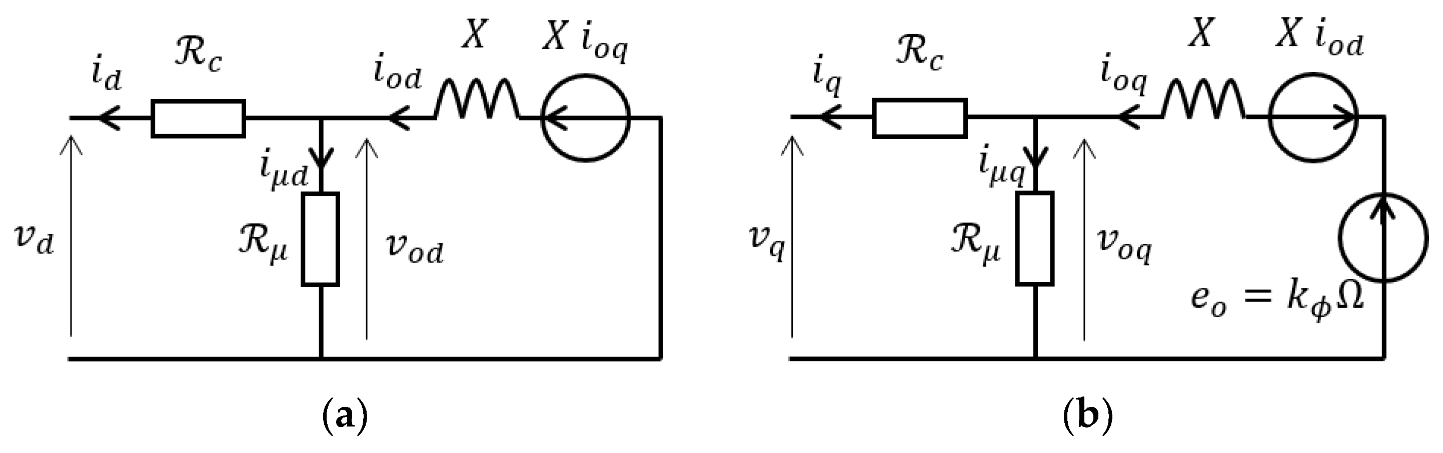
The presented methodology is based on the d–q axis equivalent circuit model taking iron losses into account via the iron loss resistance (see Figure 1) [13,14].
The optimization parameters can be categorized into three groups as follows:
- The time-dependent control variables are the d–q axis currents and . In our method, they will be analytically expressed for the two control strategies considered.
- The rotor variable , the magnitude of the air-gap flux density created by the magnets represented in the circuit via the electromotive force . It will be optimized analytically to minimize the energy losses for the considered working cycle. Note that the magnets are sized (shape and remanence) afterwards, from .
The proposed optimization method is performed in three steps.
In step 1, for the FW control, the optimal current that minimizes the total electric losses for each working point is expressed analytically. For the MTPA control, this current is zero. For both of these controls, the -axis current is directly imposed by the torque. The analytical expressions of the currents allow to express as a function of the other optimization parameters, so that
In step 2, from the previous expression of the optimal flux density that minimizes the energy losses is analytically expressed, allowing to express as a function of the remaining optimization parameters as
In step 3, a genetic algorithm is used to minimize both the energy losses obtained in step 2 and the mass of the generator.
Let us note that, with the elimination of the time-dependent optimization parameters and in the objective function , the computation time is significantly reduced to an acceptable value (a few minutes), while it would have been of several months otherwise.
2.1. Basics Equations
Due to the high inertia of the turbine, speed and torque variations are very slow. Thus, it is possible to neglect the terms in d/dt, which means that, from a sizing point of view, the machine operation can be seen as a succession of static points. Then, the main equations, such as the d–q axis stator voltages (, ) and the electromagnetic power (), can be expressed as
The expression of the copper losses is given by
with
From (1)–(6), the copper losses, for a given power and a given speed , can be expressed as follows:
For the iron losses, we have:
From (1), (2) and (8) it is possible to write
2.2. Analytical Expressions of - and -Axis Currents
The optimal currents allow the generator to satisfy the requested power and speed For a surface mounted PMSG, the q-axis current is directly imposed by the electromagnetic power. According to (3), whatever the control strategy (MTPA or flux weakening controls), this current is expressed as follows:
In an MTPA control, the d-axis current is zero:
In an FW control, the d-axis current, that minimizes both the copper losses and the iron losses, can be analytically expressed. It’s possible to show that
where the terms and depend on the resistances and the reactance as follows:
2.3. Analytical Expression of
The magnitude of the flux density produced by the magnets in the air-gap is constant during the cycle. This parameter is then optimized by the minimization of the energy losses over the cycle. With (see (21)), it is possible to express optimal expression of the magnet flux density.
In an MTPA control, since (7), (9), (10) and (11), the lost energy can be written as
Then, the flux density that minimizes the energy losses for the MTPA control is
In an FW current control, since (7), (9), (10) and (12), the lost energy can be written as
Then, the flux density that minimizes the energy losses for the MTPA control is:
2.4. Analytical Expression of Energy Losses
Finally, in an MTPA control, given (15) and (16), the expression of the lost energy is
and in an FW control, given (17) and (18), the expression of the lost energy is
In Equations (19) and (20), the remaining optimization variables are the geometrical ones (). Such an expression can be thereby minimized by the use of a genetic algorithm without an excessive computation time.
3. Modeling
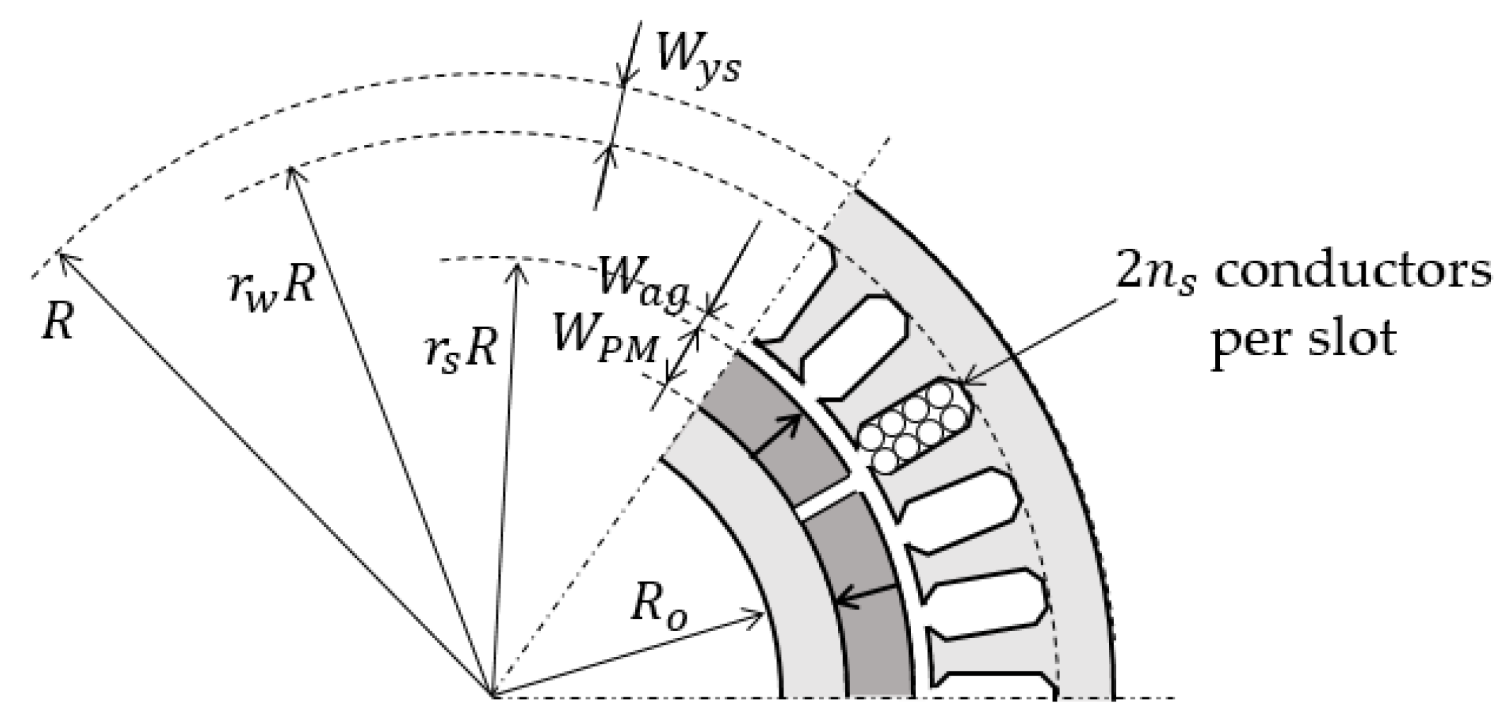
We consider a q-phase surface mounted permanent magnet synchronous generator. A 1D magnetic model is used, with steel parts assumed infinitely permeable. The winding is concentrated with one slot/pole/phase and the slots are assumed skewed by one slot pitch to reduce the torque ripple. The slot width to slot pitch ratio is 0.6. We also neglect losses in permanent magnets, assuming it is possible to reduce significantly their impact by the use of segmented magnets. The design, with only one pole pair represented, is shown in Figure 2.
3.1. Electromagnetic Model
The back-emf is proportional to which can be written as
The iron loss resistance can be deduced from (8); for phases:
where is the magnitude of the voltage, which can be expressed from the magnitude of the resulting flux density in the air-gap as follows:
The iron losses (eddy currents + hysteresis) can be also written as a function of , as described in [15], such as
with
Thus, from (20)–(23), it follows that
The winding resistance () of a -phase machine can be written as
where is the coefficient that corrects the active length due to the end windings and the slot fill factor. For the synchronous reactance of a q-phase PMSG it is possible to show that
3.2. Mass Calulcation
Only the mass of the active parts will be considered here. , and are, respectively, the mass of the copper, the mass of the iron and the mass of the magnets. They are calculated as follows:
In the proposed design, the electric magnet pole arc is set to . 180° and the magnet thickness to airgap thickness ratio is set to 7/3.
3.3. Thermal Constraint
During operation, the hottest point in the machine must remain smaller than the maximum permissible temperature in the winding , such as:
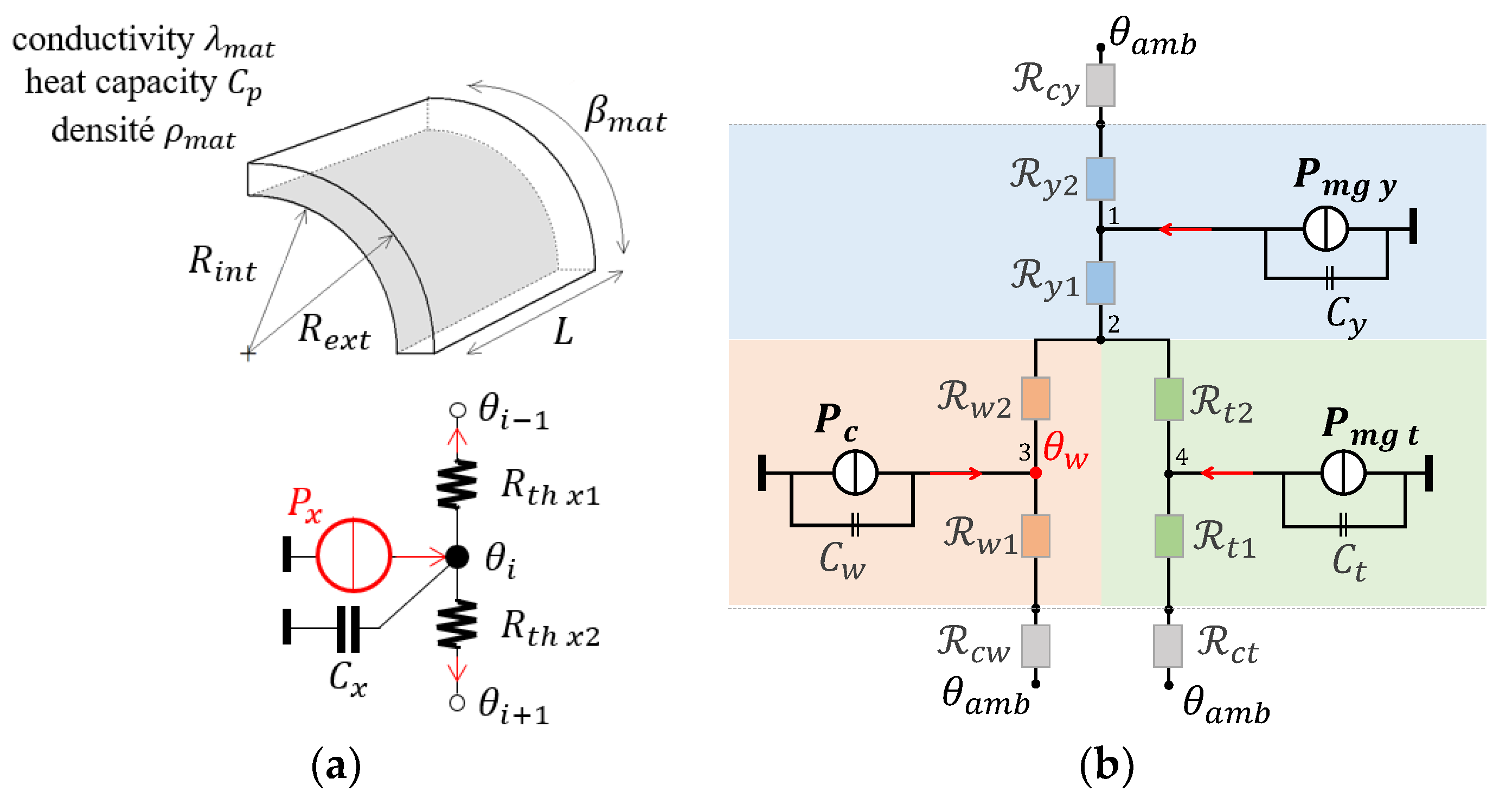
For each evaluated machine, the dynamic behavior of the temperature in the winding is calculated from the lumped parameter thermal model represented in Figure 3b [16,17]. In this study, the heat flow is assumed unidirectional in the radial direction and each cylindrical element can be modeled by an equivalent circuit, as shown in Figure 3a. The thermal resistance, as well as the thermal capacity, is calculated from the geometry and the thermal properties of the materials via (33)–(35). At the internal radius and at the external radius , the heat is extracted by convection with, respectively, = 10 (for a natural convection) and 100 W/m2K (for air cooled convection). The time-dependent temperature at node is evaluated with (36).
where is heat generated inside the element.
3.4. Saturation Constraint
The maximum flux densities in the yoke and teeth must be limited at the saturation level, such as
3.5. Electrical Constraint
We consider a voltage limit imposed by the power electronics converter. This voltage depends on the topology of the power converter and the voltage rating of the power semiconductor devices. The two-level, back-to-back voltage source converter (BTB 2L-VSC) is mostly used in the wind turbines for powers up to a few megawatts [18]. However, in the 10 MW range and above, the increase in voltage, current and losses (switching losses) requires an increase in the number of components and the number of levels. Among all the proposed converter topologies, the three-level active neutral-point diode clamped converter (3L-NPC) is one of the most popular [19]. Without going into the optimization of the power converter, which will be the subject of a future work, we impose a maximum phase voltage of 3000 V, which would be authorized by the use of medium voltage IGBT transistors (up to 6.5 kV) [20]. For -phases machines, the voltage limitation is formulated as
3.6. Mechanical Constraints
Due to severe mechanical stresses, the obtained designs must respect minimum yoke and tooth thicknesses, or the stresses will be transferred to the structural components [21]. Today, these constraints are the main limitation in the scale-up in off-shore wind power and the manufacturers do not communicate these data, which are strategic. As a consequence, the academic literature presents a lot of dispersion in the proposed constraints values and designs. For example, for a power of 10 MW, the minimum thickness of the stator yoke observed in papers varies between 14 mm and 109 mm and the minimum width of the teeth varies between 15.3 mm and 50 mm. On the basis of these observations, we set these values at 40 mm and 20 mm, respectively [22,23]. The slot depth to tooth width ratio is also limited to 8 [24]. Concerning the outer radius , setting a maximum value is more difficult, especially because the smallest radii do not necessarily lead to the lowest masses, here [25]. According to [21], if the external diameter is too large, the stress on the mechanical structure becomes too great. Consequently, according to the observed values, we will limit the space requirement by limiting the outer radius to 5 m.
4. Design Optimization
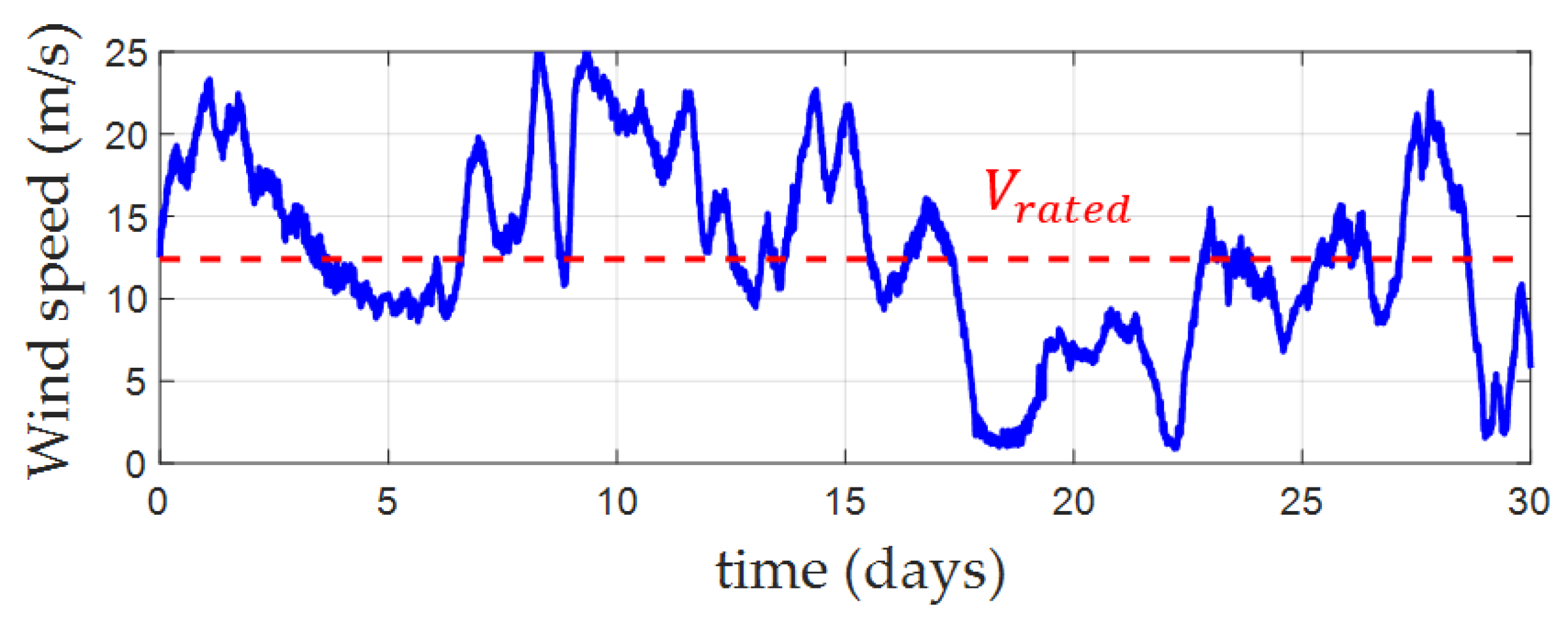
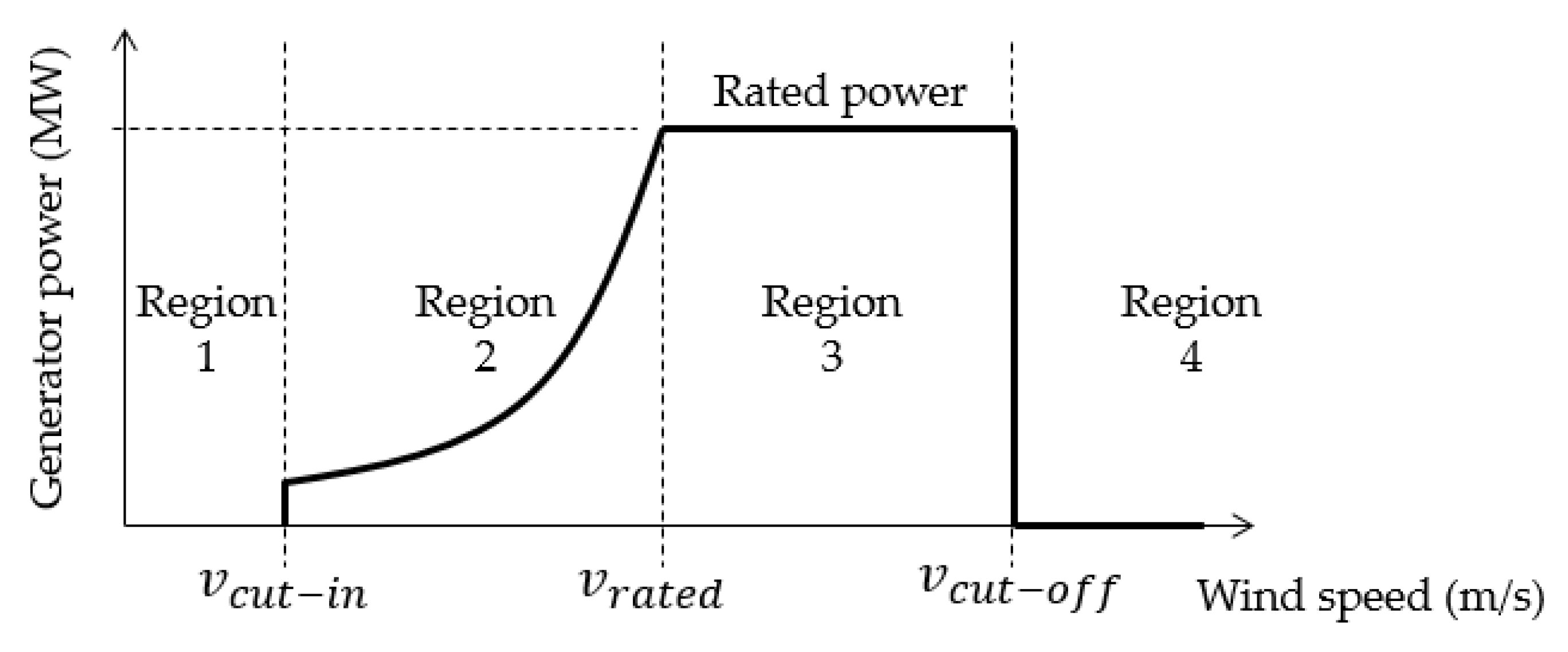
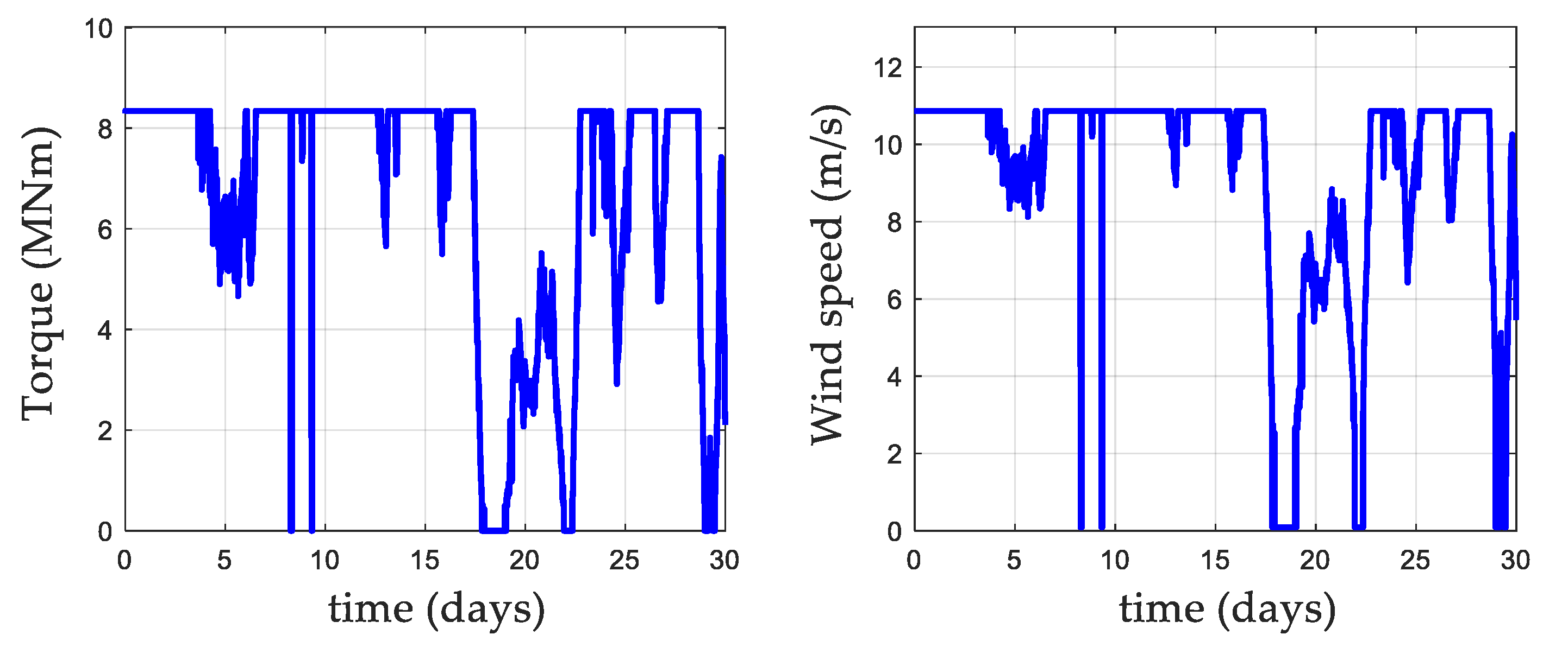
In this section, the methodology previously presented is applied to design a direct-drive PMSG for a 10 MW wind turbine (see specifications given in Table 1). A wind speed profile of 4500 points (one point every 10 min), measured in the North Sea during one month, will be considered (Figure 4) [26]. The case of a three-bladed pitch-regulated variable speed wind turbine is considered in this study. It operates at the maximum power point between a cut-in wind speed of 2.5 m/s and a rated wind speed of 12.4 m/s. Above this speed, the maximum power is limited and kept constant.
The speed and power profiles of the PMSG can be deduced from the wind speed profile and the specifications of the wind turbine, considering the four different operation modes [27] of the wind turbine, as represented in Figure 5.
In the second region, between and the rated speed , the maximum power point tracking approach (MPPT) is adopted in order to maximize the captured power [28]. In the third region, the pitch angle is regulated to limit the turbine output power. The rotor speed and the output power in this region are constants and equal to their rated values. Finally, the speed and torque profiles of the generator can be obtained; these are presented in Figure 6.
The main constant parameters used for the optimization are summarized in Table 2. The optimization parameters are listed in Table 3.
4.1. Results
The NGSAII algorithm is used to solve the two objective functions:
Note that the method proposed in this paper would also minimize the cost of the generator, either by replacing the second objective function or by adding a third objective function. In this paper, we have only chosen to minimize the mass of the generator, without minimizing its cost. According to [21], this criterion is indeed essential, today, in a context of increasing wind turbine power. However, we will present the detailed costs of the two lightest generators obtained for the two considered control strategies.
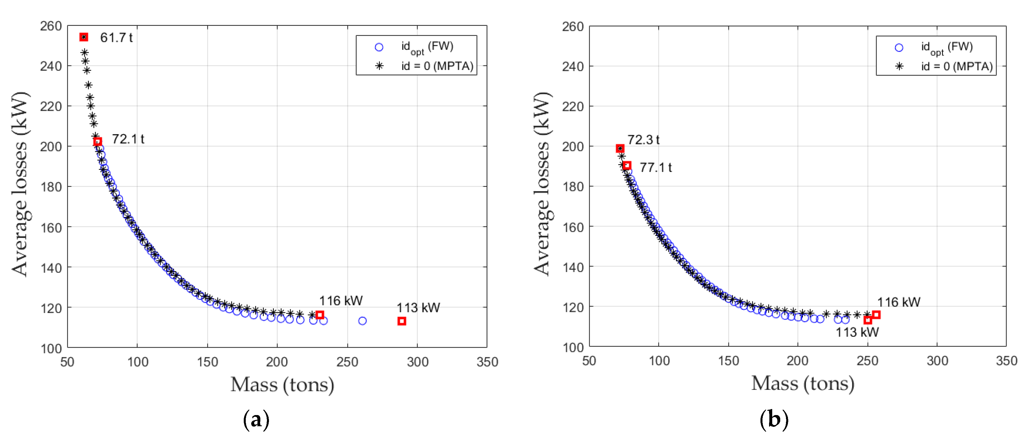
In order to analyze the effect of the number of phases, Figure 7 presents the Pareto-optimal fronts obtained when the number of phases was fixed at three and five. For both cases, the two current mode controls (FW and MTPA) were considered. The NSGA II algorithm developed by [29] and available in a Matlab code [30] was used with a number of generations and a population size of, respectively, 3000 and 500.
According to the results, for a given number of phases, the optimal Pareto fronts are overlaid. However, it can be seen that the minimum mass is always obtained for the MTPA current mode control. The result shows how the current mode control can impact the result (performance and design) of the machine when it is taken into account in the optimization process. For a three-phase machine, the variation is closed to 15%. Regarding the number of phases, the optimum is obtained for = 3. As represented in Figure 7, the mass of the machine increase with . This result is mainly due to the reduction of the pole pair number with because of the limitation of maximum number of possible slots at a given slot width. However, the increase of allows to reduce the phase current, which is necessary to reduce the constraints and the losses in the power converter when more powerful machines are investigated.
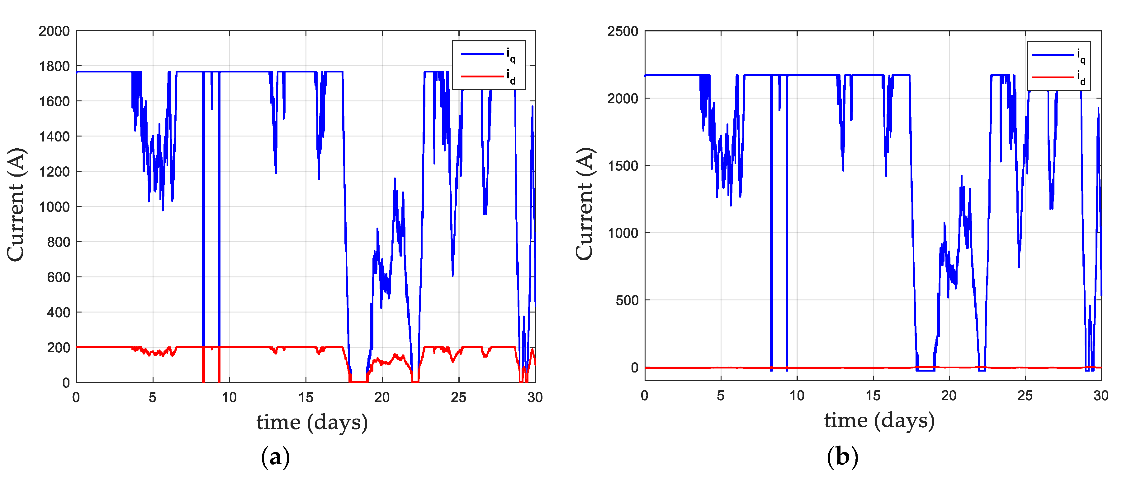
Figure 8 represents the profile of the currents and during the cycle for the lightest three-phase machine only. In the case of the FW current mode control, the current is adjusted at each working point to minimize the electrical power losses according to (12).
In Table 4, the costs of the four lightest machines presented in Figure 7 are given for comparison. The following material costs were considered [25]: 50 EUR/kg for the magnets, 3 EUR/kg for iron and 15 EUR/kg for copper. As it can be seen, machines optimized considering a MTPA control are less expensive compared to the machines optimized considering an FW control (28% and 18% for and , respectively). Such a result is mainly due to the volume of magnets, lower for the MTPA, which represents a significant part of the cost of the machine. This difference is in agreement with (16) and (18), where is lower than .
4.2. Optimal Machine
For high power offshore wind turbines, mechanical constraints strongly affect the design of the machines. To satisfy the safety of the structure, it is important to limit the mass of the nacelle to be as low as possible. Therefore, here, we consider the lower mass machine, i.e., the lower masse machine with = 3 optimized for an MTPA current mode control. In this particular case, and only because the steady state thermal regime is reached, we find the result obtained by classical methods only when the mass is minimized considering the rated power with an MTPA control. Beside the fact that it is an element of validation of the proposed method, it is important to note that an optimization for the rated power with a steady-state thermal regime not reached (which was not obvious in advance) would lead to oversizing the machine.
Table 5 summarizes the optimal geometry of the optimal generator.
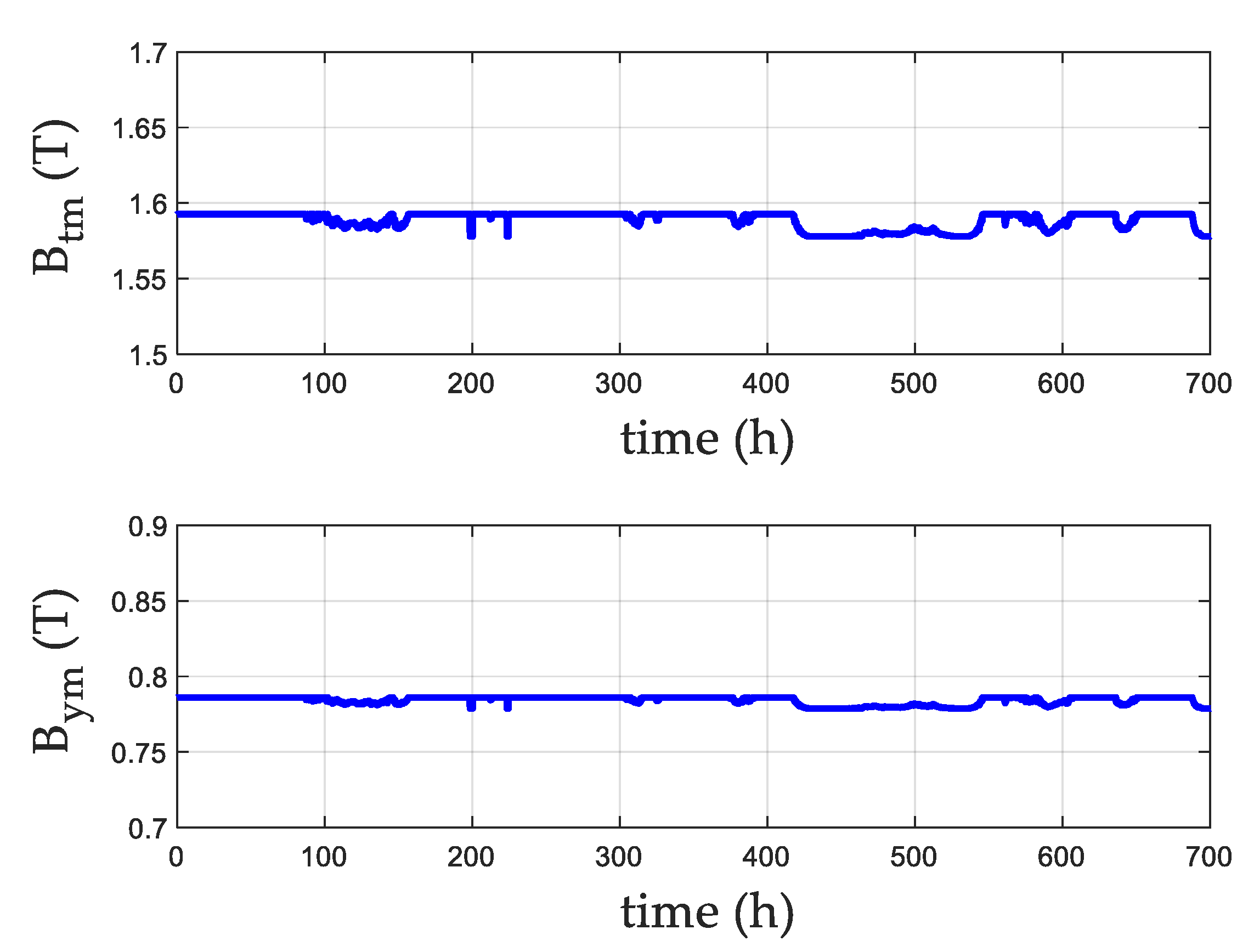
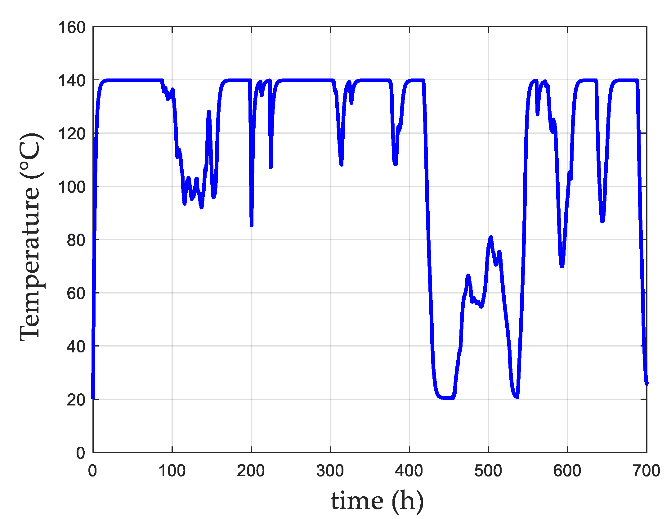
Figure 9 and Figure 10 show the flux densities and the temperature in the winding during the cycle for the optimal machine. Magnetic and thermal constraints are always fulfilled with the control of the thermal transient regime. Here, due to long operating times, the permanent thermal regime is reached. It should be noted that, for some applications (tidal turbine for example), where the steady state thermal regime is not reached, the optimization method presented in this article would avoid an oversizing of the generator.
4.3. FEA Validation
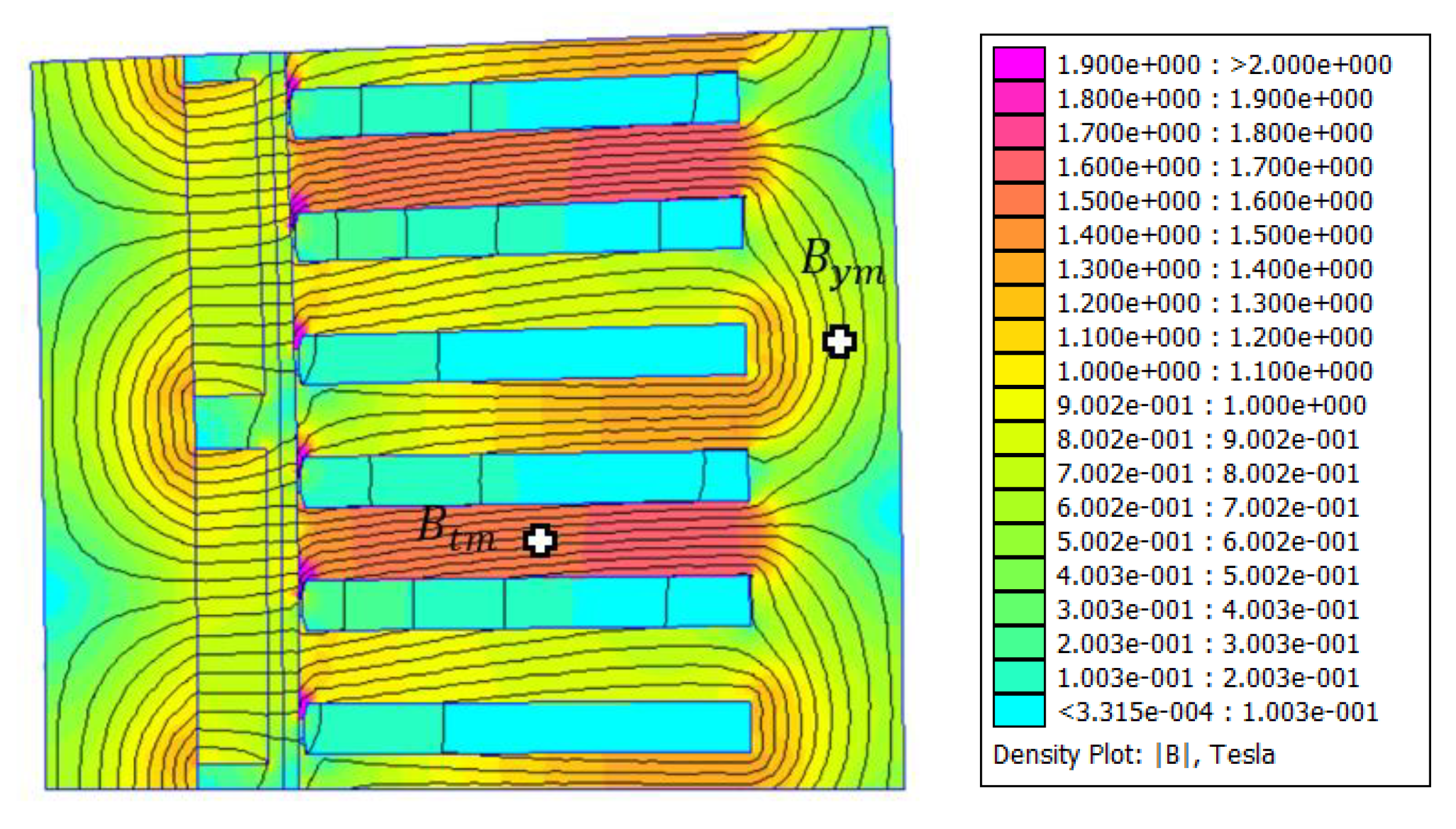
In this part, the results for the optimum generator are validated by a 2D finite element analysis (FEA). Figure 11 shows the flux lines and flux density in the optimal machine at the rated torque with the current . The average torque obtained validates the analytical model with a variation lower than 10% (see Table 6). The magnitude of the flux densities, measured in the middle of the most saturated teeth and in the middle of the yoke (see Figure 11), also validates the analytical model.
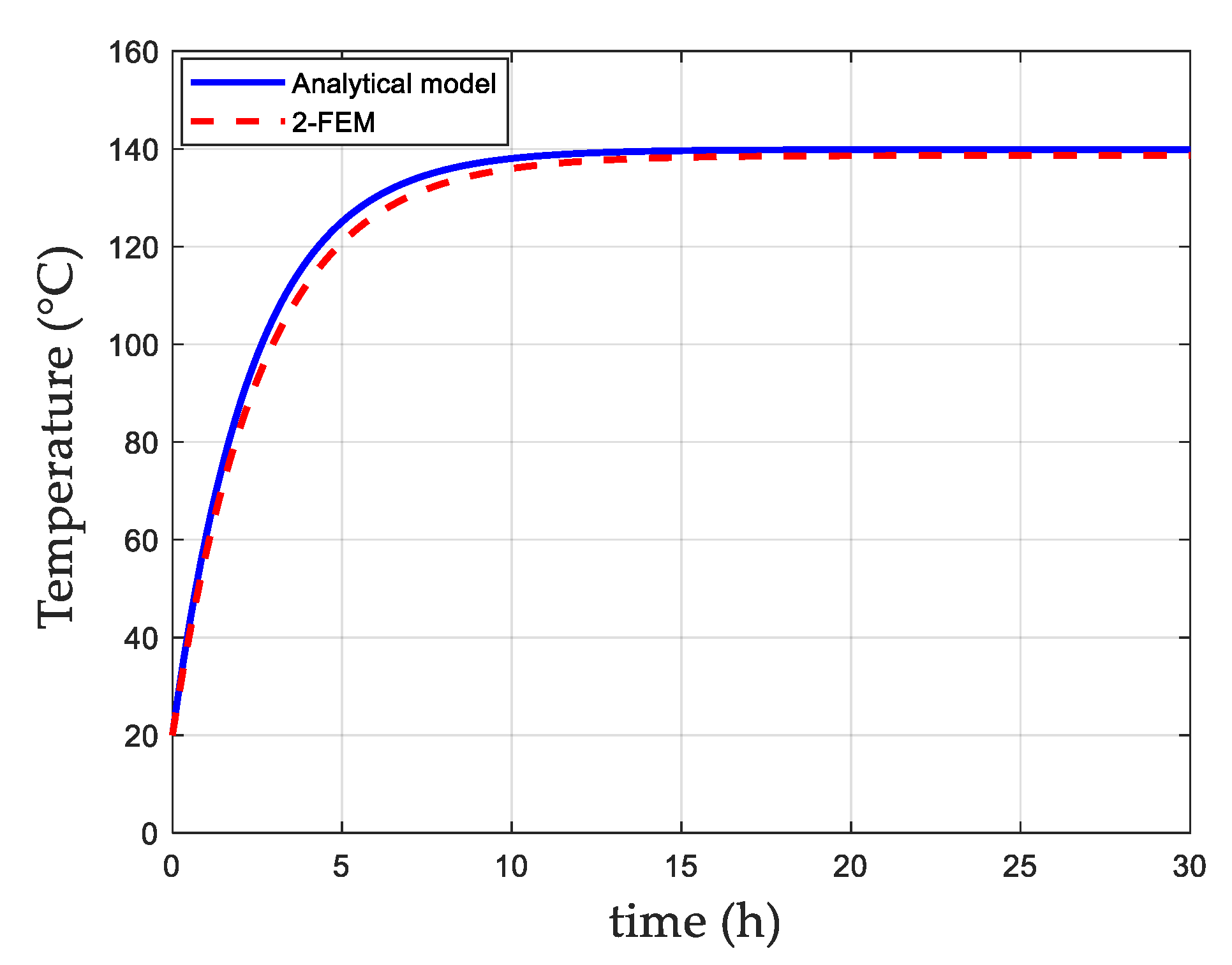
In order to validate the thermal model and its transient regime, the evolution of the temperature in the winding was calculated considering a step of power (see Figure 12) with copper and iron losses in the yoke and tooth (see Table 7) at full load, for . The result shows that both the transient and the final temperature in the winding are in good agreement.
5. Conclusions
In this paper, we showed how to take into account all the operating points of a working cycle with the control strategy in the optimization process of a PMSG. It should be noted that, by its formulation, this method is also applicable to other kinds of machines, either synchronous (with or without magnets, with or without salience) or variable reluctance machine. Contrary to “classical” methods, which reduce the problem to a few significant points of the working cycle in order to reduce the computation time, the method presented in this paper allows to consider all the points, which makes it possible to control the constraints at any point of the cycle, in particular the thermal one, characterized by a transient regime. The 1D model used was validated by a 2D finite element analysis. The dynamic thermal behavior is also controlled, avoiding an oversizing of the machine in case the permanent thermal regime is not reached. Finally, this approach, with its quickness and simplicity, constitutes a first step toward a design optimization of the complete turbine system, including the power electronics components, which will be discussed in future works.
6. Patents
Author Contributions
Conceptualization, L.D., S.O.S., R.S. and N.B.; methodology, L.D., S.O.S., R.S. and N.B.; software, L.D. and N.B.; validation, L.D., S.O.S., R.S. and N.B.; formal analysis, L.D. and N.B.; investigation, L.D. and N.B.; resources, N.B.; data curation, L.D. and N.B.; writing—original draft preparation, L.D. and N.B.; writing—review and editing, N.B.; visualization, N.B.; supervision, N.B.; project administration, N.B.; funding acquisition, N.B. All authors have read and agreed to the published version of the manuscript.
Funding
This work was carried out within the framework of the WEAMEC, West Atlantic Marine Energy Community, and with funding from the Pays de la Loire Region of France, under the OCEOS project. https://www.weamec.fr/en/projects/oceos/.
Institutional Review Board Statement
Not applicable.
Informed Consent Statement
Not applicable.
Data Availability Statement
Not applicable.
Conflicts of Interest
The authors declare no conflict of interest.
Abbreviations
| , | d-and q- axis terminal voltages (V) |
| , | d- and q- axis currents (A) |
| back electromotive force (V) | |
| armature resistance (Ω) | |
| iron loss resistance (Ω) | |
| synchronous reactance | |
| copper losses (W) | |
| iron losses (W) | |
| additional iron loss coefficient | |
| eddy currents specific loss coefficient | |
| hysteresis specific loss coefficient | |
| slot fill factor | |
| tooth opening to the slot pitch ratio | |
| coefficient for correcting the active length | |
| active length | |
| length to outer stator radius ratio | |
| outer stator radius | |
| inner rotor radius (m) | |
| inner stator radius | |
| outer rotor radius | |
| reduced inner stator radius | |
| outer winding radius | |
| reduced outer winding radius | |
| air-gap thickness | |
| magnetic airgap (magnet + mechanical airgap) (m) | |
| permanent magnet height (m) | |
| slot width (m) | |
| armature yoke thickness (m) | |
| permanent magnet width (m) | |
| number of turns per phase per pole | |
| number of pole pairs | |
| number of phases | |
| electrical magnet pole arc (rad) | |
| electric conductivity | |
| machine mechanical angular velocity (rad/s) | |
| maximal permissible temperature (°C) | |
| temperature in the copper (°C) | |
| ambient temperature (°C) | |
| heat transfer coefficient (W/m2K) | |
| copper density (kg/m3) | |
| steel density (kg/m3) | |
| permanent magnet density (kg/m3) | |
| specific heat capacity of copper (J/Kg/K) | |
| specific heat capacity of steel (J/Kg/K) |
References
- Dhar, M.K.; Thasfiquzzaman, M.; Dhar, R.K.; Ahmed, M.T.; Al Mohsin, A. Study on pitch angle control of a variable speed wind turbine using different control strategies. In Proceedings of the 2017 IEEE International Conference on Power, Control, Signals and Instrumentation Engineering (ICPCSI-2017), Chennai, India, 21–22 September 2017; pp. 285–290. [Google Scholar]
- Xin, W.; Ceng, S.; Yong, L.; Xin, L.; Bin, Q.; Wang, X. The key control technologies in the direct drive PMSG offshore wind turbine system. In Proceedings of the 27th Chinese Control and Decision Conference (2015 CCDC), Qingdao, China, 23–25 May 2015; pp. 5058–5063. [Google Scholar]
- Stuebig, C.; Seibel, A.; Schleicher, K.; Haberjan, L.; Kloepzig, M.; Ponick, B. Electromagnetic design of a 10 MW permanent magnet synchronous generator for wind turbine application. In Proceedings of the 2015 IEEE International Electric Machines & Drives Conference (IEMDC), Coeur d’Alene, ID, USA, 10–13 May 2015; pp. 1202–1208. [Google Scholar]
- Wang, J.; Qu, R.; Tang, Y.; Liu, Y.; Zhang, B.; He, J.; Zhu, Z.; Fang, H.; Su, L. Design of a Superconducting Synchronous Generator With LTS Field Windings for 12 MW Offshore Direct-Drive Wind Turbines. IEEE Trans. Ind. Electron. 2015, 63, 1618–1628. [Google Scholar] [CrossRef]
- Moghadam, F.K.; Nejad, A.R. Evaluation of PMSG-based drivetrain technologies for 10-MW floating offshore wind turbines: Pros and cons in a life cycle perspective. Wind. Energy 2020, 23, 1542–1563. [Google Scholar] [CrossRef]
- Sethuraman, L.; Maness, M.; Dykes, K. Optimized Generator Designs for the DTU 10-MW Offshore Wind Turbine using GeneratorSE. In Proceedings of the 35th Wind Energy Symposium, Grapevine, TX, USA, 9–13 January 2017. [Google Scholar] [CrossRef] [Green Version]
- Dang, L.; Bernard, N.; Bracikowski, N.; Berthiau, G. Design Optimization with Flux Weakening of High-Speed PMSM for Electrical Vehicle Considering the Driving Cycle. IEEE Trans. Ind. Electron. 2017, 64, 9834–9843. [Google Scholar] [CrossRef]
- Kalt, S.; Wolff, S.; Lienkamp, M. Impact of Electric Machine Design Parameters and Loss Types on Driving Cycle Efficiency. In Proceedings of the 2019 8th International Conference on Power Science and Engineering (ICPSE), Dublin, Ireland, 2–4 December 2019; pp. 6–12. [Google Scholar]
- Lazari, P.; Member, S.; Wang, J.; Member, S.; Chen, L. A Computationally Efficient Design Technique for Electric-Vehicle Traction Machines. IEEE Trans. Ind. Appl. 2014, 50, 3203–3213. [Google Scholar] [CrossRef]
- Li, Q.; Fan, T.; Wen, X.; Li, Y.; Wang, Z.; Guo, J. Design optimization of interior permanent magnet sychronous machines for traction application over a given driving cycle. In Proceedings of the IECON 2017–43rd Annual Conference of the IEEE Industrial Electronics Society, Beijing, China, 5–8 November 2017; pp. 1900–1904. [Google Scholar]
- Fatemi, A.; Demerdash, N.A.O.; Nehl, T.W.; Ionel, D.M. Large-Scale Design Optimization of PM Machines Over a Target Operating Cycle. IEEE Trans. Ind. Appl. 2016, 52, 3772–3782. [Google Scholar] [CrossRef]
- Dang, L.; Samb, S.O.; Bernard, N. Design optimization of a direct-drive PMSG considering the torque-speed profile Application for Offshore wind energy. In Proceedings of the 2020 International Conference on Electrical Machines (ICEM), Gothenburg, Sweden, 23–26 August 2020; pp. 1875–1881. [Google Scholar]
- Urasaki, N.; Senjyu, T.; Uezato, K. A novel calculation method for iron loss resistance suitable in modeling permanent-magnet synchronous motors. IEEE Trans. Energy Convers. 2003, 18, 41–47. [Google Scholar] [CrossRef]
- Zhang, H.; Dou, M.; Deng, J. Loss-Minimization Strategy of Nonsinusoidal Back EMF PMSM in Multiple Synchronous Reference Frames. IEEE Trans. Power Electron. 2019, 35, 8335–8346. [Google Scholar] [CrossRef]
- Bernard, N.; Missoum, R.; Dang, L.; Bekka, N.; Ben Ahmed, H.; Zaim, M.E.-H. Design Methodology for High-Speed Permanent Magnet Synchronous Machines. IEEE Trans. Energy Convers. 2016, 31, 477–485. [Google Scholar] [CrossRef] [Green Version]
- Mellor, P.; Roberts, D.; Turner, D. Lumped parameter thermal model for electrical machines of TEFC design. IEE Proc. B Electr. Power Appl. 1991, 138, 205–218. [Google Scholar] [CrossRef]
- Bernard, N.; Ahmed, H.B.; Multon, B.; Kerzreho, C.; Delamare, J.; Faure, F. Flywheel energy storage systems in hybrid and distributed electricity generation. In Proceedings of the PCIM 2003, Nuremberg, Gemany, 22–24 May 2003. [Google Scholar]
- Yaramasu, V.; Wu, B.; Sen, P.C.; Kouro, S.; Narimani, M. High-power wind energy conversion systems: State-of-the-art and emerging technologies. Proc. IEEE 2015, 103, 740–788. [Google Scholar] [CrossRef]
- Blaabjerg, F.; Ma, K. Wind Energy Systems. Proc. IEEE 2017, 105, 2116–2131. [Google Scholar]
- Chivite-Zabalza, J.; Larrazabal, I.; Zubimendi, I.; Aurtenetxea, S.; Zabaleta, M. Multi-megawatt wind turbine converter configurations suitable for off-shore applications, combining 3-L NPC PEBBs. In Proceedings of the 2013 IEEE Energy Conversion Congress and Exposition, Denver, CO, USA, 15–19 September 2013; pp. 2635–2640. [Google Scholar] [CrossRef]
- Shrestha, G.B.; Polinder, H.; Ferreira, J. Scaling laws for direct drive generators in wind turbines. In Proceedings of the 2009 IEEE International Electric Machines and Drives Conference, Miami, FL, USA, 3–6 May 2009; pp. 797–803. [Google Scholar]
- Polinder, H.; Bang, D.; Van Rooij, R.; McDonald, A.; Mueller, M. 10 MW Wind Turbine Direct-Drive Generator Design with Pitch or Active Speed Stall Control. In Proceedings of the 2007 IEEE International Electric Machines & Drives Conference, Antalya, Turkey, 3–5 May 2007; Volume 2, pp. 1390–1395. [Google Scholar]
- Damiano, A.; Marongiu, I.; Monni, A.; Porru, M. Design of a 10 MW multi-phase PM synchronous generator for direct-drive wind turbines. In Proceedings of the IECON 2013—39th Annual Conference of the IEEE Industrial Electronics Society, Vienna, Austria, 10–13 November 2013; pp. 5266–5270. [Google Scholar]
- Li, H.; Chen, Z.; Polinder, H. Optimization of Multibrid Permanent-Magnet Wind Generator Systems. IEEE Trans. Energy Convers. 2009, 24, 82–92. [Google Scholar] [CrossRef]
- Liu, D.; Polinder, H.; Abrahamsen, A.B.; Wang, X.; Ferreira, A.J. Comparison of Superconducting Generators and Permanent Magnet Generators for 10-MW Direct-Drive Wind Turbines. In Proceedings of the 19th International Conference on Electrical Machines and Systems (ICEMS), Chiba, Japan, 13–16 November 2016. [Google Scholar]
- Available online: https://vortexfdc.com/ (accessed on 9 December 2019).
- Sohoni, V.; Gupta, S.C.; Nema, R.K. A Critical Review on Wind Turbine Power Curve Modelling Techniques and Their Applications in Wind Based Energy Systems. J. Energy 2016, 2016, 1–18. [Google Scholar] [CrossRef] [Green Version]
- Kim, K.-H.; Van, T.L.; Lee, D.-C.; Song, S.-H.; Kim, E.-H. Maximum Output Power Tracking Control in Variable-Speed Wind Turbine Systems Considering Rotor Inertial Power. IEEE Trans. Ind. Electron. 2012, 60, 3207–3217. [Google Scholar] [CrossRef]
- Kalyanmoy, D.; Amrit, P.; Sameer, A.; Meyarivan, T. A Fast and Elitist Multiobjective Genetic Algorithm: NSGA II. IEEE Trans Evol. Comput. 2002, 6, 182–197. [Google Scholar]
- Available online: https://fr.mathworks.com/matlabcentral/fileexchange/49806-matlab-code-for-constrained-nsga-ii-dr-s-baskar-s-tamilselvi-and-p-r-varshini (accessed on 9 November 2019).
Figure 1.
(a) d-axis equivalent circuit; (b) q-axis equivalent circuit.

Figure 2.
Design and geometric parameters of the PMSG.

Figure 3.
(a) Thermal equivalent circuit of a cylindrical element; (b) lumped parameter thermal model of PMSG.
Figure 3.
(a) Thermal equivalent circuit of a cylindrical element; (b) lumped parameter thermal model of PMSG.

Figure 4.
Wind speed profile measured at the North Sea in January.

Figure 5.
Typical power curve of a pitch-controlled wind turbine.

Figure 6.
Speed-torque profiles for the generator.

Figure 7.
Pareto-optimal front of optimal machines for (a) and (b).

Figure 8.
Evolution of the optimal d–q axis currents for : FW (a) and MTPA (b).

Figure 9.
Evolution of the maximum flux density in tooth and yoke of the optimal generator.

Figure 10.
Evolution of the temperature in the winding.

Figure 11.
Flux lines and flux density at full load.

Figure 12.
Evolution of the temperature in the winding at the maximal power.


Table 1.
Specifications of the considered wind turbine.
| Parameters | Values |
|---|---|
| Blade radius | 82 m |
| Maximal power | 10 MW |
| Cut-in speed | 2.5 m/s |
| Rated speed | 12 m/s |
| Cut-out wind speed | 25 m/s |
Table 2.
Constant parameters.
| Parameters | Values |
|---|---|
| 1.6 T | |
| 2.5 kV | |
| 20 mm | |
| 40 mm | |
| 2 | |
| 0.035 | |
| 30 | |
| 10 W/m2k | |
| 100 W/m2k | |
| 140 °C | |
| 20 °C | |
| 8960 Kg/m3 | |
| 7800 Kg/m3 | |
| 7600 Kg/m3 | |
| 390 J/Kg/K |
Table 3.
Optimization parameters.
| Parameters | Min | Max |
|---|---|---|
| 20 | 200 | |
| 0 | 1 | |
| 0 | 1 | |
| 2 | 5 | |
| 0.2 | 0.6 | |
| 10 mm | 100 mm | |
| 1/2 | 10 |
Table 4.
Cost of the optimal solutions.
| q = 3 | q = 5 | |||
|---|---|---|---|---|
| FW | MTPA | FW | MTPA | |
| Cost of magnets (kEUR) | 371 | 218 | 458 | 311 |
| Cost of iron (kEUR) | 135 | 126 | 141 | 138 |
| Cost of copper (kEUR) | 296 | 228 | 315 | 299 |
| Total material cost (kEUR) | 802 | 572 | 914 | 748 |
Table 5.
Optimal machine parameters.
| Parameter | Value |
|---|---|
| 3 | |
| 156 | |
| 5 m | |
| 1.15 m (0.23) | |
| 0.968 | |
| 0.992 | |
| 1.2 T | |
| 1 T | |
| 1.59 T | |
| 0.79 T | |
| 8 mm | |
| 18.7 mm | |
| Total active material weight | 61.75 tons |
| Iron weight | 42.2 tons |
| Copper weight | 15.2 tons |
| Magnet weight | 4.36 tons |
| Average losses | 253 kW |
| 2990 V | |
| 1030 A | |
| 0.98 |
Table 6.
Maximum torque and EMF at 10 MW and 11 rpm.
| Quantity | Analytical Model | FEA | Variation |
|---|---|---|---|
| 1.59 | 1.6 | 0.7% | |
| 0.79 | 0.84 | 6.3 | |
| Torque (MNm) | 8.6 | 8.13 | 5.47% |
| Magnitude of the EMF (1st harmonic) (kV) | 3.02 | 2.96 | 2% |
Table 7.
Losses of the optimal generator at the maximal power (10 MW, 1.03 kA).
| Analytical Model | FEA | Variation | |
|---|---|---|---|
| Iron losses in the yoke | 20 kW | 13 kW | −35% |
| Iron losses in the teeth | 139 kW | 173 kW | 25% |
| Total iron of the stator | 159 kW | 163kW | 3% |
| Copper losses | 173 kW | ||
Publisher’s Note: MDPI stays neutral with regard to jurisdictional claims in published maps and institutional affiliations. |
© 2021 by the authors. Licensee MDPI, Basel, Switzerland. This article is an open access article distributed under the terms and conditions of the Creative Commons Attribution (CC BY) license (https://creativecommons.org/licenses/by/4.0/).
Share and Cite
MDPI and ACS Style
Dang, L.; Ousmane Samb, S.; Sadou, R.; Bernard, N. Co-Design Optimization of Direct Drive PMSGs for Offshore Wind Turbines Based on Wind Speed Profile. Energies 2021, 14, 4486. https://0-doi-org.brum.beds.ac.uk/10.3390/en14154486
AMA Style
Dang L, Ousmane Samb S, Sadou R, Bernard N. Co-Design Optimization of Direct Drive PMSGs for Offshore Wind Turbines Based on Wind Speed Profile. Energies. 2021; 14(15):4486. https://0-doi-org.brum.beds.ac.uk/10.3390/en14154486
Chicago/Turabian StyleDang, Linh, Serigne Ousmane Samb, Ryad Sadou, and Nicolas Bernard. 2021. "Co-Design Optimization of Direct Drive PMSGs for Offshore Wind Turbines Based on Wind Speed Profile" Energies 14, no. 15: 4486. https://0-doi-org.brum.beds.ac.uk/10.3390/en14154486
Note that from the first issue of 2016, this journal uses article numbers instead of page numbers. See further details here.