Prediction of Climate Change Effect on Outdoor Thermal Comfort in Arid Region

Abstract

Climate change and expected weather patterns in the long-term threaten the livelihood inside oases settlements in arid lands, particularly under the recurring heat waves during the harsh months. This paper investigates the impact of climate change on the outdoor thermal comfort within a multifamily housing neighborhood that is considered the most common residential archetype in Algerian Sahara, under extreme weather conditions in the summer season, in the long-term. It focuses on assessing the outdoor thermal comfort in the long-term, based on the Perceived Temperature index (PT), using simulation software ENVI-met and calculation model RayMan. Three different stations in situ were conducted and combined with TMY weather datasets for 2020 and the IPCC future projections: A1B, A2, B1 for 2050, and 2080. The results are performed from two different perspectives: to investigate how heat stress evolution undergoes climate change from 2020 till 2080; and for the development of a mathematical algorithm to predict the outdoor thermal comfort values in short-term, medium-term and long-term durations. The results indicate a gradual increase in PT index values, starting from 2020 and progressively elevated to 2080 during the summer season, which refers to an extreme thermal heat-stress level with differences in PT index averages between 2020 and 2050 (+5.9 °C), and 2080 (+7.7 °C), meaning no comfortable thermal stress zone expected during 2080. This study gives urban climate researchers, architects, designers and urban planners several insights into predicted climate circumstances and their impacts on outdoor thermal comfort for the long-term under extreme weather conditions, in order to take preventive measures for the cities’ planning in the arid regions.

1. Introduction

Due to rapid urbanization, the global population is migrating from rural to urban areas. This change is meanly observed during the previous few decades [1]. Therefore, city-induced climate change has serious repercussions on public outdoor activities, health and tourism. Researchers have been increasingly interested in studying the negative effects of urbanization on thermal sensation and conditions inside cities [2,3]. The oases settlements that are the most common urban patterns in the Saharan region in North Africa face an enormous urban sprawl, especially in the last few decades. These regions showed a high reclamation on thermal qualities throughout the cities, especially during summer. Many centuries ago, urban know-how was adapted to the local conditions found in the vernacular and traditional architecture and their resilience over time [4,5]. On the contrary, in recent summer days, a large human lethargy is made due to the thermal environment and people prefer to remain indoors and only venture outside for key activities such as economic activities and commuting. Simultaneously, non-obligatory activities such as walking, sightseeing or socializing become less favorable [6]. Despite the use of developed building’s means and new materials’ generation, the current urban strategies implemented within local authorities are mainly unadaptable to climate change. The situation increases thermal discomfort inside the oases settlements, and occupants claim more thermal stress during the hot season. Consequently, thermal adaptation patterns look at the climate change fluctuations for short-term, medium-term and long-term variations and adapt cities to the weather and weather conditions, specifically in the arid regions. Moreover, to envisage future climate change for impact and adaptation assessment, several probable future anthropogenic greenhouse-gas-emissions-based socioeconomic storylines were established by the Intergovernmental Panel for Climate Change (IPCC) [7,8].

Therefore, this study aims to promote long-term predictions for outdoor thermal comfort through a unique urban multifamily residential typology, specifically inside the oases settlements in Southern Algeria, that can yield valuable insights for various urban planning strategies. We used state-of-the-art urban climate modelling tools to assess outdoor thermal comfort levels through the study context. Moreover, the findings of this research can allow architects and urban planners, authorities and programmers to benefit from environmental and urban strategies. In the Saharan urban environments, outdoor thermal comfort assessment is imperative to understand people’s well-being and reduce negative impacts during extreme events, such as heatwaves and heat stress. Therefore, this paper aimed to quantify outdoor thermal comfort under current and future weather projections from 2020 until 2080 and generate an algorithm for thermal stress predictions. More specifically, the following questions are answered:

• What are the outdoor thermal comfort levels inside a multifamily residential neighborhood concerning IPCC emission scenarios?
• How severe will be the impact of climate change on outdoor thermal comfort during summer by 2080?
• How to generate an algorithm for hourly and yearly predictions of outdoor thermal comfort thresholds through similar spatial–climate conditions?

The main objectives are to quantify the outdoor thermal comfort inside a most common urban archetype across the oases territories following an empirical approach and investigate the long-term heat stress patterns under the climate change conditions. A background, as well as an introduction of the study context, highlights the objectives and the obtained results which were presented through the study. Moreover, numerical modeling, measurements in site, a literature review and a reference case excerpt are presented. A comparison of seven different weather data projections was made to stand by the future patterns of outdoor thermal comfort in Algerian arid lands settlements. Levels of heat stress were analyzed, and the results were used to generate an algorithm for the outdoor thermal comfort predictions. Finally, recommendations for future work are outlined.

2. Literature Review

Our literature review covers more than 100 publications found on Scopus and the Web of Science that are relevant to the field of thermal comfort levels and their predictions in the long-term. Therefore, we selected the most relevant publications to our research topic aiming towards a new scientific re-thinking about the outdoor thermal comfort variations and their long-term patterns under climate change conditions.

The current article presents a definition framework based on reviewing various studies, including climate change scenarios [9], outdoor thermal comfort evaluation [10] and urban climate modeling [11]. One of the challenges of this study is to provide predictions of thermal comfort on an urban scale beyond what is taken in the literature, which mainly addresses the definition of thermal comfort predictions on a building scale. We reviewed most studies investigating relationships among “climate change” and “thermal heat stress” through urban livability [12] for short-term and long-term durations. Most of the future weather files used to predict the impacts of climate change are performed on building performance; we cited the most relevant works on this that have been published [8,13,14,15,16,17,18,19,20].

The adaptive comfort model [21,22,23,24] considers that people’s thermal sensation mainly depends on microclimatic parameters, i.e., air temperature, humidity, radiant temperature, wind and solar radiation. It further includes individuals’ characteristics and situations, such as age, gender, clothing, activity and subjective issues, such as behaviors, expectations and acclimatization [11]. Accordingly, outdoor thermal comfort studies were performed for long years. They developed several methods and human thermal indices [25,26], to quantify the thermal comfort levels against climate change and urban phenomena such as Urban Heat Island (UHI). In the foregoing research, Yaglou and Minard., 1957, developed the “wet-bulb globe thermometer” index based on the total heat stress introduced by physical exercise, radiation and temperature, humidity and wind on human bodies through three military camps [27]. Their work was followed by developing the “Discomfort index” (DI) by Thom, 1959 [28]. More recently, the outdoor thermal comfort is investigated based on newly developed thermal indices performed basically through multi-criteria related to the close environment and persons, such as the “Physiologically Equivalent Temperature” (PET) which was developed by Hoppe in 1999 [29]. PET is defined as an air temperature in a specific indoor environment no submitted to wind and solar radiation influences, in which the human body’s heat budget could be balanced basically with similar skin and core temperature under the evaluated outdoor conditions. Moreover, the “Perceived Temperature” (PT) is defined as a constant state model that describes the thermal perception of an individual considering the air temperature of a reference environment, where the thermal perception would be similar as in the actual conditions [10,30,31,32,33,34]. The thermo-physiological modelling of (PT) index is based on the Klima Michel Model (KMM) [35,36,37]. In another context, Jae-Young et al., 2008 [38] examined the outdoor thermal comfort in the Korean Peninsula in 2007 using (PT) index. The distribution of (PT) showed that it might be a useful thermal index for assessing thermal comfort and thermal stress through the Korean Peninsula. In their study, Dae-Guen et al. (2010) [39] investigated the relationship between (PT) index variations and the daily excess mortality in Seoul, South Korea, between 1991 and 2005. In another study, Wang and Zhu (2020) [40] explored the impact of global warming on the perceived temperature (PT), which the authors consider as the most relevant thermal index for the outdoor thermal comfort quantification under extreme climate change.

On the other hand, only limited studies were investigated considering climate change and its long-term impacts on outdoor heat stress levels, such as the study conducted by Fang et al., 2021 [41] in Guangzhou, China. The air temperature has the most significant effect on thermal sensation, according to the results. In colder or warmer conditions, the mean thermal sensation vote with an increase in clothing insulation. With different thermal indices, Cheung and Hart, 2014 [42] utilized the universal thermal comfort index (UTCI) to evaluate the outdoor thermal comfort in Hong Kong for the long-term duration from 1971 to 2100, based on two emissions scenarios (A1B and B1) developed by the IPCC reports. Comparing the early calculated UTCI (based on observation data) and forthcoming UTCI, the results showed that the future climate projections have elevated behavior and greater peak value. Taking a different approach, Liu et al. (2018) [43] demonstrated that CFD simulation of wind conditions could be used to assess outdoor thermal comfort in the future planning stage without being coupled with thermal simulation. Additionally, in the study of Nazarian et al. (2017) [44], researchers tried to introduce an improved methodology of predicting outdoor thermal comfort and its spatial variability in urban streets. Kariminia et al. (2011) [45] searched on the basis of PET index to formulate the suitable thermal comfort range relevant for an urban context in temperate and dry climate zones to ensure human activities throughout the outdoor spaces.

Eventually, the added value of this work is not only to address long-term thermal issues in arid regions but also to extend results to several climate zones in Algeria for further studies.

3. Methodology

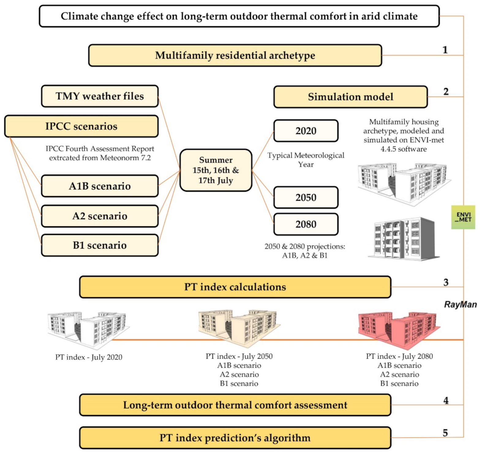
The research methodology resulted in the calculation and prediction approach of the outdoor thermal comfort among multifamily residential housing in the arid region of Southern Algeria. The used calculation method is based on the simulations’ approach applied to the validated model of the multifamily residential housing. On the other hand, the purpose of calculations is to generate a mathematical algorithm for future outdoor thermal comfort in long-term patterns. Figure 1 illustrates the detailed conceptual framework of the study describing the steps of the research methodology.

3.1. Multifamily Residential Archetype

According to Semahi et al., 2020 [46], the residential sector presents the large buildings’ category in Algeria. Even more, the Algerian residential sector comprises two main typologies: (i) multifamily housing, which presents 51% of the total residential buildings, and (ii) single-family houses, which presents 49% of the residential buildings. Several apartment buildings’ types concerning the multifamily housing typologies depend on the contract type that reflects the inhabitants’ income (free promotional housing, rental ownership housing, participatory public housing and public rental housing) [46]. The social residential buildings category (public rental housing) represents a significant part of (31%) multifamily housing. The number of apartments in the social housing building category has increased every year. In 2008, the Algerian Ministry of Housing, Urbanism and the City launched a program to construct 800,000 apartments between 2009 and 2014 and 800,000 apartments between 2015 and 2019. This study evaluates the outdoor thermal comfort levels’ evolution depending on climate change within a multifamily housing neighborhood, which presents the most common archetype residential typology in Algeria.

3.2. IPCC Scenarios and Weather Files Criteria

Following several studies looking into climate change, this study focuses on methods and approaches related to the long-term pattern in climate change. The Intergovernmental Panel on Climate Change (IPCC) is an intergovernmental organization of the United Nations, which was established in 1988 by the World Meteorological Organization (WMO). IPCC provides the world with objective, scientific information to understand the scientific factors of the risk of human-induced climate change, its economic and natural political impacts and risks, and potential response options [47,48]. Furthermore, IPCC established long-term emission scenarios which have been widely adopted in the study of potential climate change, its impacts and opportunities to reduce climate change [7]. The methods estimating the evolution of climate change within the Global Climate Models (GCMs) are numerical models of the physical processes that characterise the global climate system, comprising the atmosphere, oceans, cryosphere and land surface. Conferring to the Fourth Assessment Report of the IPCC (AR4) [49], the buildings sector has the most significant potential for climate change mitigation, and the development of mitigation when the adaptation strategies become a key challenge for building professionals [20,23,50,51]. The current work explores the IPCC emission based on the Meteonorm database [52], which presents a stochastic weather data generator and a spatial interpolation tool. Therefore, the study is based on EPW files for representing the Typical Meteorological Year (TMY) [53], and three IPCC emission scenarios, which are A1B, A2, and B1, reveal the three projection’s weather files available on Meteonorm 7.2 and used in the current study. Among several climate change studies, Calvin Cheung and Hart, 2014 [42]; Richter, 2016 [54]; Carter, 2018 [55]; Moazami et al., 2019 [8]; Nematchoua et al., 2019 [15]; and other researchers used in their work the emission scenarios for the climate-change adaptation models.

Based on the literature review, it is identified that a limited number of studies investigated the impact of climate change on outdoor thermal comfort based on future weather projections. On the other hand, many similar studies were carried based on the building scale extreme weather adaptation. Meteonorm as a weather generator tool, applies the GCMs of the IPCC Fourth Assessment Report (AR4) and the climate data recorded in typical weather files (TMY). Moreover, it generates different formats of future weather files for a ten-year time period between 2010 and 2100. The three used projections were generated for the years 2050 and 2080, depending on the study area’s context and geographical coordinates. These scenarios are based on a specific storyline highlighting the main relationships, characteristics and dynamics, between the key driving forces: population, land use, agriculture, economy, energy and technology.

The storylines represent various demographic, social, economic, technological and environmental developments [7,20]. The main characteristics of all different scenarios and storylines are explained in

Table 1. IPCC climate change scenarios and storylines.

Storyline	Characteristics
A1 A1F1, A1T, A1B	An accelerated economic development; Important rise of the world population which reaches its peak in mid-century and relapses after that; Fast establishment of developed strategies and more effective technologies; The principal themes are convergence towards regional actions, building capacity, and enhanced cultural and social interactions; A1 family scenario occurs into three groups that describe alternative trends of technological development in the energy system: A1F1 (fossil intensive), A1T (non-fossil sources) and A1B (balanced across all energy sources).
A2	Very heterogeneous world; The principal theme is self-sustenance and maintenance of local identities; Regional fertility patterns converge very slowly; World population is continuously increasing; The economic development is strongly aligned towards regional actions; The economic development and technological change are more dispersed and slower compared to other storylines.
B1	Converging world; Rise of the global population which peaks in mid-century and lower after that; A significant economic orientation towards a service and information economy; The use of clean and resource-efficient technologies versus the decrease in material intensity; Worldwide solutions to economic, social and environmental sustainability contributing improved equity, without adaptation of climate strategies.
B2	World in which the fundamental focus is on local economic, social and environmental sustainability solutions; The global population is continuously augmented at a rate lower than A2 storyline; Economic development at medium level; Slower and more diverse technological development compared to the B1 and A1 scenarios; Oriented toward social equity and environmental control and management; Special attention toward regional and local level development.

.

Firstly, the work aimed to compare the current thermal levels (2020) based on (TMY) versus the future projections in 2050 and 2080 (A1B, A2 and B1). The study was performed exclusively in the summer season, and the assessed days were 15, 16 and 17 July during each evaluated period. The chosen days of the study represent the hot season, and July is considered the warmest month of the year in Algeria [56,57,58]. Hence, we tried to spread the simulation time over 72 h of running simulation for the accuracy of the results.

Furthermore, the evaluation of the outdoor thermal comfort was performed based on the perceived temperature index (PT) defined by VDI (2008) [59], Staiger et al. (2012) [30] and Jendritzky et al. (2000) [32].

Table 2. The physiological meaning of PT index [32].

Perceived Temperature (°C)	Thermal Perception	Physiological Stress
<−39	Very cold	Extreme cold stress
−39 to −26	Cold	Heavy cold stress
−26 to −13	Cool	Moderate cold stress
−13 to 0	Slightly cool	Low cold stress
0 to +20	Comfortable	Comfort possible
+20 to +26	Slightly warm	Low heat load
+26 to + 32	Warm	Moderate heat load
+32 to +38	Hot	Heavy heat load
>+38	Very Hot	Extreme heat load

shows the PT index values and the thermo-physiological meaning.

The purpose is to formulate a mathematical equation (algorithm) for the future yearly predictions of PT index values for (BWh) climate conditions. As identified by Guan, 2009 [19], the projections of temperatures have the highest confidence among all the climatic variables. In contrast, the level of uncertainty is higher for humidity, wind and solar radiation.

Neighborhood Context

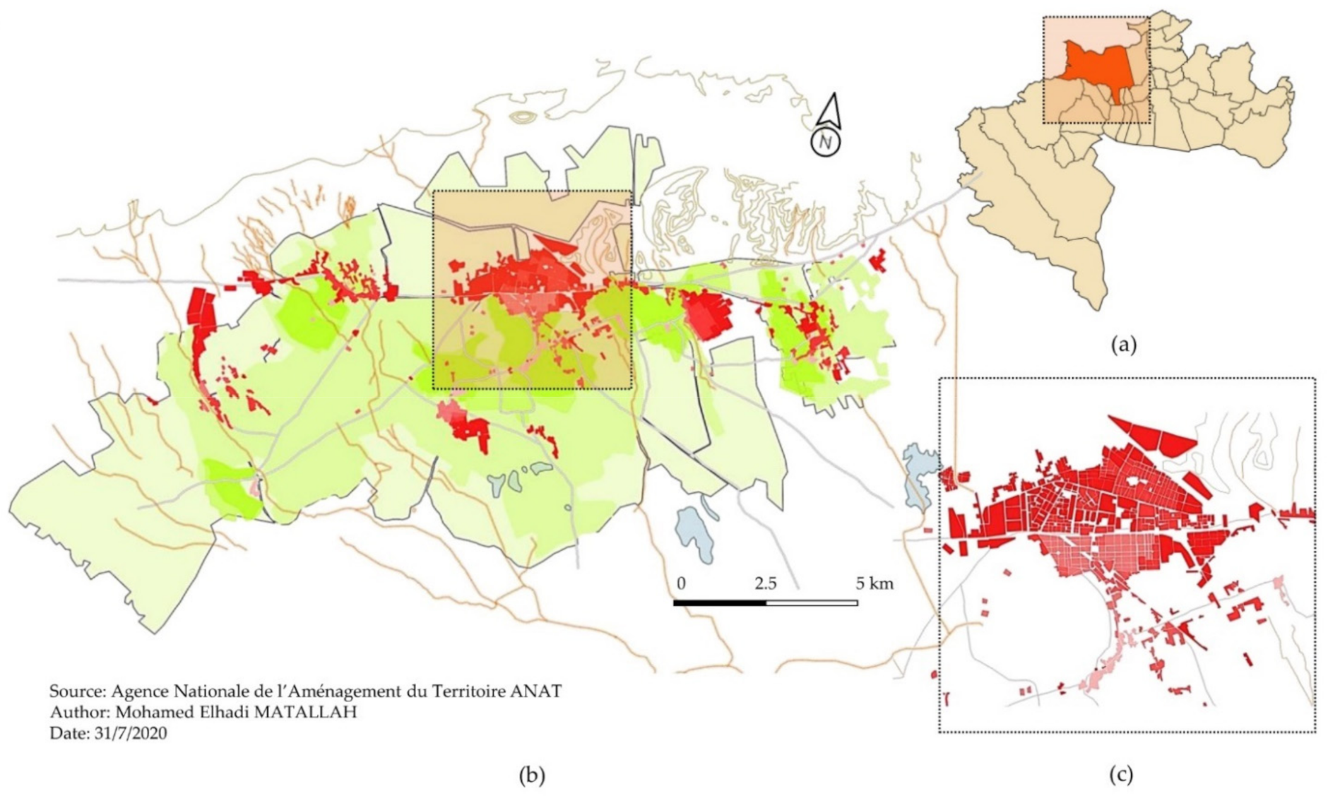
The study context is located in the Tolga Oases Complex, considered as one of the largest livable oases territories in North Africa (Figure 2).

The work is conducted throughout the Tolga Oases Complex territory (34°43′00″ N and 5°23′00″ E) located in Biskra Province, Southern Algeria [58,60]. Moreover, the chosen multifamily housing neighborhood represents a typical social residential building which was taken as a representative model for this study (

Table 3. Selected multifamily housing neighborhood and urban pattern.

Multifamily building’s configuration
Ground plan and 3D view
Multifamily housing mass				Buildings are composed of three floors, with a similar height of 12.50 m
				20 % of the building’s mass presents the open surfaces ‘windows and doors’
				Built-up occupancy is equal to 18% compared to total unbuilt surface
Building materials properties	Wall		Hollow brick, mortar, plaster						Concrete, mortar
	Roof		Concrete slab, mortar, polystyrene, plaster
	Thermal conductivity (W/m-K)		Hollow brick: 0.48; Concrete: 1.75; plaster: 0.35; mortar: 1.15
		SVF = 0.87						SVF = 0.78			SVF = 0.64
		-						H/W = 1			H/W = 0.89
		SDmax = 15: 30 h						SDmax = 15: 30 h			SDmax = 15: 30 h
ENVI-met modelling parameters	Building	Brick wall (aerated), lightweight concrete
	Soil	Asphalt, Pavement: concrete pavement grey, Natural surface: loamy soil
	Vegetation	spherical (small trunk. sparse. small (5 m)); Grass: 50 cm aver. dense
3D model
	Block model (ArchiCAD 22 software)				Architectural model (ArchiCAD 22 software)					Simulation model (ENVI-met 4.4.5 software)

). The selected apartment building consists of four stories of this archetype building. Each level is subdivided into two dwellings with an area of 64 m² approximately for a single-family dwelling. The neighborhood includes 150 dwellings divided into 11 separate building blocks. The neighborhood is located in the centre of Tolga city. It has a unified geometry design with fragmented blocks, built with identical height (H = 12.50 m), moderate urban compactness and a very low built occupancy: 18% [61]. It is essential to indicate that the site is missing urban vegetation arrangements, where only very limited green areas, “grass”, and few trees, Ficus rubiginosa, are spontaneously planted. The building design has a rectangular form with a close similarity in design proprieties throughout the dwellings’ blocks.

However, it is necessary to state that the current study focuses specifically on the neighborhood’s spatial configuration as opposed to the parametric characteristics and building materials.

The selected site comprises several building forms (Figure 3). The building is equivalent to 06 residential blocks (M₁) (including two dwellings in each level). Overall, the multifamily housing neighborhood includes several adjacent modules that lead to other modules’ composition (M₂) (two adjacent buildings). The (M)’s items are only illustrated to clarify the spatial configuration throughout the investigated site. The site represents a common urban geometry for the residential sector, specifically for the multifamily housing design in Algeria.

Furthermore, the construction strategies, materials, shading, and technical systems used depend strongly on the national or local context, availability and prices of materials, climate, traditions and national building legislation [20].

3.3. Simulation Model and Outdoor Thermal Comfort Assessment

Possibly, the choice of weather data is considered the most important input for urban climate simulation in the context of climate change. The current research is based on EPW-files generated by Meteonorm 7.2 database (https://meteonorm.com/en/; accessed on 15 March 2021) [60] for TMY weather files and future projections to the year 2080, which were taken from the World Meteorological Organization (WMO) [8]. Meteonorm 7.2 database uses the IPCC Fourth Assessment Report (AR4) as a model to allow the climate change projections. Meteonorm is limited only to three scenarios: A1B, A2 and B1. Meteonorm tool is universally used for climate change studies. Instead of climate values, the IPCC results (AR4) are utilized as input. The deviations of parameters global radiation, temperature and precipitation and the three scenarios (A1B, A2 and B1) were included. With the combination of Meteonorm’s current database 1961–1990, the stochastic generation and the typical years’ interpolation algorithms can be calculated for any location for different scenarios between 2010 and 2100 [52]. Furthermore, based on the analysis of variations of temperature, precipitations and global radiation of year to year, month to month and the ten past years, as well as climate model forecasts by Meteonorm, an autoregressive model was synthesized to generate a realistic monthly time series of future projections. The study outputs are determined using a simulation model created in ENVI-met 4.4.5 software (https://www.envi-met.com/; accessed on 10 October 2020) [62,63,64] and RayMan 3.1 Beta [33,34] calculation model to calculate the PT index.

The simulated model is calibrated based on monitored data. Root mean square error (RMSE) and mean bias error (MBE) indices were used to confirm the calibration [65]. The validated model focused on how closely the simulated results match the monitored data. The monitoring was performed on 15 and 16 July 2014. Moreover, to validate the numerical model, we needed 48 h of running simulation as sufficient time for the three monitored points of the conducted site (

Table 4. Summary of validation of the simulated model in ENVI-met software.

Neighborhood	Indices	Point 1		Point 2		Point 3
Multifamily housing	RMSE	2.92	8.75%	2.98	8.96%	3.75	10.70%
	MBE	−0.36	1.08%	−0.44	1.31%	−1.99	5.67%

). The validation was performed based on the hourly datasets. The following equations were applied to check the calibration of the simulated model.

$$\mathrm{RMSE}=\sqrt{\frac{1}{\mathrm{n}}·{\displaystyle \sum }_{\mathrm{i}=1}^{\mathrm{n}}{\left({\mathrm{Sim}}_{\mathrm{i}}-{\mathrm{Obs}}_{\mathrm{i}}\right)}^2}$$

(1)

$$\mathrm{MBE}=\frac{1}{\mathrm{n}}·{\displaystyle \sum }_{\mathrm{i}=1}^{\mathrm{n}}\left({\mathrm{Sim}}_{\mathrm{i}}-{\mathrm{Obs}}_{\mathrm{i}}\right)$$

(2)

In the above equations, Equations (1) and (2), Sim and Obs are the simulated and observed (measured) data, respectively, and “n” represents the number of the data values used for the calculation. As defined in ASHRAE Guideline 14-2014 [66], the simulation model is considered validated if the following conditions are met:

The hourly (MBE) values are within ±10%, and hourly (RMSE) values are below 30%. In this research, hourly data were used for the validation of the numerical model.

We coupled ENVI-met 4.4.5 and RayMan 3.1 Beta to have an accurate calculation of the PT thermal index. The requested microclimatic outputs are air temperature (Tair), relative humidity (RH), air velocity (Vair) and the mean radiant temperature (Tmrt) of the three investigated days 15, 16 and 17 July. Therefore, only microclimatic outputs of future scenarios were taken, while the TMY outputs were performed in the study of Matallah et al. (2021) and mentioned in Matallah’s study report, 2020 [65].

On the other hand, using the future weather data projections can induce limitations regarding the confidence level in predicting different microclimatic parameters applied in building simulation. We are required to state that the current study seeks to develop an algorithm (greedy algorithm) [67,68] for PT index predictions. Additionally, the applied algorithm refers only to similar housing typologies, similar climate conditions, same lands (Tolga Oases Complex or Biskra Province) and summer season, which makes other neighborhoods’ typologies or climate zones different study area’s context not adequate for the algorithm application. Accordingly, the algorithm could be used to improve urban design management under extreme weather conditions due to global climate change, notably during the summer season through the arid lands. Moreover, the algorithm presents a simple equation of variables such as the predictions’ years and hours. The algorithm could be applied under the programming method in climate software such as ENVI-met and EnergyPlus databases.

4. Results

This section combines two parts of the analyzed datasets between results and their interpretations. Moreover, results include, in particular, the elaboration process of the PT index prediction algorithm when the data analysis in these sections shows the three points results (

Table 5. PT index values in point 1 among three periods: 2020, 2050 and 2080.

Time	TMY 2020			A1B Scenario 2050			A1B Scenario 2080				A2 Scenario 2050				A2 Scenario 2080						B1 Scenario 2050				B1 Scenario 2080
	15th	16th	17th	15th	16th	17th	15th		16th	17th	15th	16th		17th	15th	16th		17th			15th	16th	17th		15th	16th	17th
00:00	19.2	21.1	21.2	25.7	26.8	30.3	28		28.4	33.4	24.9	26.6		29.7	27.5		28.9		34.2		23.3	25.5	29.3		24.9	26.3	30.6
01:00	18.6	20.5	20.1	24.3	27.5	29.9	26.2		29.6	33	23.8	27.1		27.9	26.1		29.9		32.3		22.5	25.9	27.1		23.6	26.8	28.3
02:00	18.6	20.1	19.9	23.2	26.8	26.5	27.1		28.6	28	22.8	26		26.2	24.9		29.4		28.7		21.5	24.9	25.2		22.6	26	25.9
03:00	18.2	20.0	19.1	23.4	25.9	27	23.4		28.1	29.7	22.7	25.6		25.2	25.5		28.3		29.5		21.7	24.2	24.8		22.8	25.3	26.3
04:00	17.5	19.4	19.0	22.9	25.5	26.1	24.7		27.3	29	22.4	25.2		25.1	25.1		27.5		28.4		21.5	24	24.2		22.5	25.1	25.6
05:00	17.5	19.2	18.5	21.3	26.7	25.2	22.6		29.4	27.8	21.1	26.8		24.4	23		29		27.8		20.1	24.9	23.6		21	26.1	24.9
06:00	17.8	19.1	18.5	21.8	27.4	24.8	23		29.4	27.2	21	26.8		24.2	23.1		30.1		27.2		20.1	25.7	23.5		21	27	24.5
07:00	19.4	20.7	20.3	21.9	28.4	25.7	22.7		31	27.5	21.6	27.8		24.9	23.2		31.8		28.1		20.8	26.9	24.2		21.6	28.4	25.2
08:00	22.8	23.4	23.1	25.2	29.7	27.6	26.7		32	29.2	24.9	29.6		27.2	26.7		32.4		29.6		24	28.3	26.7		24.7	29.4	27.5
09:00	29.5	28.1	28.3	29.2	33.8	36.6	30.7		35.7	37.6	29.4	33		35.6	30.9		35.6		38.3		28.5	31.5	34.9		29.2	32.8	36
10:00	29.7	30.1	30.5	33.9	34.1	38.2	33.9		36.7	39.7	32.6	34.5		37.1	34.5		36.8		39.2		31.7	33	36.5		32.5	33.9	37.3
11:00	31.0	30.7	31.4	34.4	36.8	39.1	36.2		38.5	41.1	34.3	36		37.9	36		38.1		40.1		32.7	34	37.5		33.5	36.5	38.1
12:00	32.0	31.1	32.2	37.3	37.8	38.2	39.2		39.2	40.5	37	37.7		38.3	38.9		39.2		39.2		36.2	35.7	36.6		36.3	36.6	37.4
13:00	32.6	31.6	32.8	39.2	38.8	39.9	40.6		40.9	40.8	39	37.9		39.5	41.1		39.4		40.1		37.3	36.2	37.5		38.5	37.1	38.2
14:00	34.2	32.2	33.6	38.1	38.5	41	38.9		40.1	42.7	36.7	37.2		40.9	39.5		40.7		41.1		35.1	36.4	38.8		35.9	37.3	39.4
15:00	34.6	33.5	34.3	38.4	38.1	49	40.1		40.4	50.9	38	36.8		46.5	39.7		39.2		49.8		36.6	36.1	45.8		37.4	36.8	46.7
16:00	34.6	33.6	35.2	35.4	43	45.2	35.7		42.7	45.1	34.9	39.5		43.6	36.1		41.8		45.4		33.5	38.5	42		34.2	39.4	42.7
17:00	33.4	32.9	34.5	37	39.6	41.8	40.8		41.4	40.9	36.5	38		41	39.1		40.1		42		35.1	36.7	39.3		36.2	38.2	39.5
18:00	28.4	32.6	33.3	34.5	41	37.7	35.2		38.8	40.4	32.1	38.9		37	33.8		41.6		37.9		30.6	38.1	35.2		30.8	41.4	37.9
19:00	26.9	26.8	27.1	31.9	35.4	32.8	34.5		35.6	34.3	31	34.1		32.6	33.4		36.9		33.4		29.4	33.3	30.9		30.6	34.4	31.6
20:00	23.6	24.0	24.7	29.1	35.7	30.8	29.5		36.1	31.3	28.6	33.9		30.8	30		37.1		32		26.8	32.8	29.4		27.9	33.7	30
21:00	22.5	23.3	24.1	28.2	34.4	32.6	29.7		34.9	35	28.2	33.5		31.9	30		37.3		33.9		26.7	32.4	30.5		27.8	33.9	31.4
22:00	22.1	22.3	23.5	30.4	31.4	31.1	32.7		33.3	31.9	30.1	30.4		30.7	33.3		33.3		31.5		28.5	29.4	29.2		29.8	29.8	30.2
23:00	21.6	21.3	22.7	29.5	31.4	28.1	31.2		34.2	29.4	28.5	30.1		27.8	31.4		33.2		29		27.3	28.9	26.5		28.4	30	27.2
PT (°C)				0–20				20–26					26–32							32–38				≥38
Thermal perception				Comfortable				Slightly warm					Warm							Hot				Very Hot
Thermo-physiological stress				Comfort possible				Slight heat stress					Moderate heat stress							Great heat stress				Extreme heat stress

,

Table 6. PT index values in point 2 among three periods: 2020, 2050 and 2080.

Time	TMY 2020			A1B Scenario 2050			A1B Scenario 2080				A2 Scenario 2050				A2 Scenario 2080						B1 Scenario 2050				B1 Scenario 2080
	15th	16th	17th	15th	16th	17th	15th		16th	17th	15th	16th		17th	15th	16th		17th			15th	16th	17th		15th	16th	17th
00:00	19.2	20.9	21.0	25.1	26.6	30.9	27.3		28.5	33.9	24.4	26.3		29.3	26.9		28.6		33.6		22.9	25.2	28.7		24.3	26.7	30
01:00	18.5	20.2	20.9	24.4	27.3	30.4	25.8		29.5	33.5	24	26.6		27.9	26.3		29.4		32.7		22.6	25.4	27.5		23.8	26.6	29.2
02:00	18.4	20.0	20.1	23.2	26.5	27.4	25.4		29.1	29.8	22.7	26		27.7	24.9		28.7		29.7		21.5	24.9	25.2		22.6	25.9	26.4
03:00	17.8	19.5	19.3	23.3	26.4	27.2	25.6		29.2	29.2	23	26		27.2	25.8		29.2		29.1		21.9	24.6	24.7		23.1	26.1	26
04:00	17.3	19.4	19.2	23.3	25.6	26.8	25.7		26.9	28.6	22.7	25.1		27.1	25.5		27.5		29.1		21.6	24	24.5		22.9	25.1	25.7
05:00	16.8	19.2	18.6	21.3	26.3	25.8	22.9		28.6	27.9	20.9	25.7		26.1	23.1		28.8		28.1		19.9	24.5	24		20.9	25.7	25.2
06:00	17.9	19.0	18.5	21.7	26.4	25.3	23.5		28.8	27.8	21.2	26		25.1	23.5		29.1		28.1		20.3	24.7	23.6		21.3	26.2	24.9
07:00	18.9	20.7	20.0	21.6	28.6	26.5	22.9		31.4	28.7	21.2	27.9		25.5	23.3		31.1		29		20.3	26.7	24.7		21.2	28.3	26
08:00	22.5	23.2	23.1	25.1	31	28.2	26.2		32	30.1	25	29.6		27.9	26.5		32.4		30.5		24.1	28.2	26.9		24.9	29.4	28
09:00	25.3	25.4	25.5	29.6	32.3	37.5	31.1		34.3	39	29.2	32.1		34.6	30.9		34.9		38.7		28.1	31.1	35.2		29	32.1	36.2
10:00	26.4	27.1	27.3	33	35.1	38.4	34.9		37.8	39.1	32.6	35.3		41.5	34.5		38		38.4		31.2	33.8	36		32.1	34.8	36.8
11:00	27.7	28.2	28.8	34	37.4	41	35.5		39.5	43	33.1	35.9		40.8	35.8		38.5		40.1		32.1	34.8	39		33.8	36.1	39.9
12:00	29.2	29.1	32.5	34.8	37.6	40.8	36.7		38.6	41.8	35.3	36.5		43.2	36.9		38		40.8		33.7	35.1	38.7		34.8	36	40
13:00	32.8	31.7	32.7	38.4	39.5	41.1	40.8		41.5	41	37.4	39.3		43.9	39.7		40.8		42.2		35.8	37.4	39.2		37	38.4	40
14:00	33.9	32.7	33.7	39.5	38.5	43.2	41.5		40.3	42.7	39	37		45.5	40.9		39.4		43.4		37.3	36.4	40.5		37.8	37.3	41.2
15:00	34.1	33.6	34.4	40.4	37.8	47.7	42.3		39.1	49.6	39.6	36.8		43.4	42.3		38		47.4		38.1	34.9	43.7		39.1	35.8	45.3
16:00	30.3	30.0	32.3	34.5	42	43.7	35.1		41.9	46.7	35.6	39.5		43.5	36.4		42.3		46.6		33.7	39.3	42.3		34.5	40.5	45.1
17:00	29.8	29.8	30.6	37	38.6	41.9	39.2		38.7	41.3	35.3	37		41.7	38.1		39.4		42.9		33.7	36.4	39.8		34.8	37.3	40.5
18:00	28.2	28.5	29.4	31.6	39	40	33.5		41.3	42.2	30.7	37		43.1	32.2		38.4		40.1		29.3	35.1	36.7		30.2	36.1	37.6
19:00	27.3	26.8	27.8	32.7	34.6	34	36		36.2	34.2	32	33.1		34	34.8		34.5		33.9		30.2	31.3	31.3		31.4	32.3	32.1
20:00	24.2	24.3	25.3	30.1	36	31.9	32.3		39.1	32.5	29.6	34.8		31.8	31.5		38.3		32.6		27.8	33.6	29.8		29.4	34.7	30.5
21:00	22.9	23.5	24.9	29.2	33.5	35	31.5		35.6	38.6	28.6	34.5		34.7	30.7		38.8		37.5		27.1	33.6	33.1		28.2	35.6	34.4
22:00	22.6	22.3	24.5	31	31	32.4	33.3		32.5	34.3	29.9	30.2		33.3	33.2		32.3		32.5		28.7	28.6	30.1		30	29.8	31.2
23:00	21.8	21.7	23.3	29.3	31.7	29.6	31.1		33.3	31.3	28.3	30.8		30	31.2		34.1		30.3		27.1	29.3	27.4		28.2	30.7	28.2
PT (°C)				0–20				20–26					26–32							32–38				≥38
Thermal perception				Comfortable				Slightly warm					Warm							Hot				Very Hot
Thermo-physiological stress				Comfort possible				Slight heat stress					Moderate heat stress							Great heat stress				Extreme heat stress

and

Table 7. PT index values in point 3 among three periods: 2020, 2050 and 2080.

Time	TMY 2020			A1B Scenario 2050			A1B Scenario 2080				A2 Scenario 2050				A2 Scenario 2080						B1 Scenario 2050				B1 Scenario 2080
	15th	16th	17th	15th	16th	17th	15th		16th	17th	15th	16th		17th	15th	16th		17th			15th	16th	17th		15th	16th	17th
00:00	18.9	20.7	20.8	27.1	27	29.9	28.8		29.5	32.4	25.6	26.6		29.3	28.8		29.2		32.4		23.6	25.3	28		25.4	26.4	29.2
01:00	18.2	20.2	21.2	26.1	26.9	28.4	29		28.8	31.2	25.7	26.3		27.9	29.1		29.1		30.7		24	25.2	26.4		25.5	26.2	27.7
02:00	18.3	19.6	19.5	24.1	27.6	28.7	26.5		30.5	31.9	23.5	27.3		27.7	26.3		30.7		32.1		22.2	26.1	26.5		23	27.2	28.1
03:00	18.1	19.2	19.4	24.7	27.2	28.6	26.7		30	31.3	24.2	26.7		27.2	27		30.4		31.6		22.8	25.1	26		24.2	26.7	28
04:00	18.0	19.4	19.0	23.9	25.4	28.2	25.9		26.9	30.7	23.4	25.1		27.1	26.3		27.4		31.8		22.5	23.9	26		23.3	25.1	27.2
05:00	17.0	19.1	18.7	21.2	25.9	27.3	22.8		28.1	29.8	20.9	25.3		26.1	23.1		28.2		30.7		19.9	24.1	25.2		20.9	25.2	26.6
06:00	18.1	18.8	18.5	22.1	26.2	25.5	23.9		28.6	27.2	21.9	25.6		25.1	24		28.7		27.4		21.1	24.6	24.1		22	25.8	24.9
07:00	18.9	19.9	20.3	21.6	29.7	26	22.8		33.5	27.6	21.3	29.3		25.5	23.2		34		27.8		20.4	28	24.5		21.3	29.2	25.5
08:00	22.0	23.2	23.0	25.1	31	27.8	26.9		34.6	29.4	25.1	30.6		27.9	27.2		35		29.7		24	29.6	26.9		24.9	30.5	27.7
09:00	24.8	25.4	25.6	29.7	33.5	39	31.7		36	41	28.4	32.8		34.6	30.8		35.2		38.4		27.4	31	32.2		28.3	32.3	35
10:00	26.4	27.7	27.7	35.8	37.7	42.7	38.2		40.8	44.2	34.2	37		41.5	37.4		40.5		41.4		32.6	35.6	36.9		33.2	36.2	38.4
11:00	27.9	28.2	29.4	38.4	41.3	44.3	41		44.2	44.6	36.8	40		40.8	39.6		43.7		44.2		34.9	37.7	39.7		36.1	39.3	40.9
12:00	31.7	31.0	32.7	34.8	38.3	45	36.5		40.4	47.3	34.5	37.5		43.2	35.7		39.2		46.6		32.9	35.7	42.5		33.8	36.6	43.6
13:00	32.8	31.5	33.4	36.7	42.2	44.6	38.5		46.2	46.7	36.3	40.3		43.9	38		44.7		45.7		34.7	40.5	41.8		35.9	40.2	41.6
14:00	33.6	32.6	34.1	39.7	39.2	46.2	41.9		40.9	46.7	39.4	37.4		45.5	41.4		38.6		47.3		37.6	37.5	43.2		38.2	37.3	44.1
15:00	30.3	30.7	32.3	39.7	38.1	44.3	42.9		40.2	46.3	40.3	37.5		43.4	41.4		38.9		44.6		37.5	35.5	41.2		39.6	35.2	42.3
16:00	30.3	30.2	31.8	35	43.9	43.5	36.9		46.3	46.7	34.8	42		43.5	36.1		45.6		45.3		33	41	41.6		33.5	42.3	42.6
17:00	29.8	29.8	31.3	35.4	39.9	42.6	37.6		42.3	44.6	35.2	37.6		41.7	36.7		40.6		43.2		33.1	36.8	39.6		34.2	38.1	39.2
18:00	28.7	28.5	30.0	34.8	36.9	44	37.2		38.8	46.5	34	37		43.1	36.7		38.4		45.7		32.2	35.1	40.7		33.3	36.1	42.1
19:00	27.2	27.4	28.3	34.4	33.6	34.3	37.3		35.2	34.6	33.2	33.1		34	36		34.5		34.9		31.4	31.3	32.2		32.6	32.3	33
20:00	24.4	24.7	25.8	31.1	38.7	32.1	32.4		41.8	32.8	30.4	36.9		31.8	33.1		40.9		33.5		28.6	35.5	30.2		29.2	36.9	30.9
21:00	23.0	23.9	25.2	29.7	37.3	36.4	31.9		41.4	39.2	29.1	36.1		34.7	31.5		40.6		38.4		27.5	35.2	33.9		28.9	35.9	35.1
22:00	22.3	22.8	24.7	29.2	31.7	33.9	32		33.9	35.9	28.5	31.4		33.3	31.5		34.5		35.4		27.2	29.8	31.5		28.7	30.3	33
23:00	21.7	22.3	23.0	28	34	30.4	30.2		37	32.3	27.4	33		30	29.9		37.4		31.6		25.9	31.3	28.3		27.3	32.4	29.2
PT (°C)				0–20				20–26					26–32							32–38				≥38
Thermal perception				Comfortable				Slightly warm					Warm							Hot				Very Hot
Thermo-physiological stress				Comfort possible				Slight heat stress					Moderate heat stress							Great heat stress				Extreme heat stress

). The final equation of the algorithm is based on all data throughout the three monitored points in the site and covers the total simulated time. Therefore, the results and discussion section are divided into two parts: Section 3.1 presents the data analysis according to the simulations running and describes all the data obtained within different studied weather scenarios. Section 3.2 focuses on developing the PT index prediction algorithm through a variety of steps: PT index averages analysis, PT index trends’ forms, validation of equations and elaboration of the final model of the algorithm.

4.1. Perceived Temperature (PT) Index for Points 1, 2 and 3

PT index values during 2050 showed five different thermal zones depending on the human’s body thermal perception, which are presented from the lowest thermal stress to highest, respectively: comfortable, slightly warm, warm, hot and very hot zones. The three 2050 scenarios (Table 5) presented a close similarity in PT index values averages with PT_2050.ave = 31.6 °C; when PT_A1B-2050.ave = 32.6 °C, PT_A2-2050.ave = 31.8 °C, PT_B1-2050.ave = 30.4 °C, hot and warm thermal zones, respectively. On the other hand, 2020 average: PT_{2020 ave} = 25.7 °C in the slightly warm thermal zone. PT index values maximums through all scenarios were PT_2020.max = 35.2 °C, PT_A1B-2050.max = 49 °C, PT_A2-2050.max = 46.5 °C, PT_B1-2050.max = 45.8 °C. All of the PT index maximums were registered in point 1, while PT_max.2050 was in the hot thermal zone, and PT_max.2050 was in the very hot thermal zone.

PT index values minimums during all scenarios (Table 6) were PT_2020.min = 16.8 °C in point 2, PT_A1B-2050.min = 21.2 °C, PT_A2-2050.min = 20.9 °C and PT_B1-2050.min = 19.9 °C in point 3. While PT_min.2020 and PT_min.B1-2050 presented a comfortable thermal zone. On the other hand, PTmin-2050 for A1B and A2 scenarios are slightly warm thermal zones. The variation in thermal zones’ duration was significant, apparently between 2020 and 2050 scenarios, where the comfortable thermal was between 0:00 a.m. and 7:00 a.m. in 2020. However, 2050 showed one hour of the comfort zone at 5:00 a.m. for one day exclusively in the B1 scenario. Furthermore, the heat stress zones occupied all conducted days’ hours in 2050, which are balanced between slightly warm, warm, hot and very hot thermal zones. The very hot thermal zone was registered among daytime hours between 10:00 a.m. and 6:00 p.m.; however, 2020 did not have a very hot thermal zone.

Results showed a significant elevation on PT averages between 2020 and 2050 with a difference of +5.9 °C. Apparently, A1B presented the hottest period across all scenarios, where point 1 was all time the thermal stressful place. In comparison to all PT index values in the previous periods, 2080 scenarios showed four different thermal zones, which were slightly warm, warm, hot and very hot thermal zones. PT index averages were more elevated versus 2050 scenarios, when PT_2080.ave = 33.4 °C, PT_A1B-2080.ave = 34.5 °C, PT_A2-2080.ave = 34.2 °C in the hot thermal zone and PT_B1-2080.ave = 31.5 °C in the warm thermal zone. On the other hand, the PT index maximums of the 2080s three scenarios presented a slight elevation comparing to 2050 scenarios (+1.9 °C) and a significant elevation to 2020 (+15.7 °C), while PT_A1B-2080.max = 50.9 °C, PT_A2-2080.max = 49.8 °C and PT_B1-2080.max = 46.7 °C, all the values were registered in the three points included in the very hot thermal zone. Otherwise, PT index minimums were PT_A1B-2080.min = 22.6 °C in point 1, PT_A2-2080.min = 23 °C in point 1 and PT_B1-2080.min = 20.9 °C in points 2 and 3, which were in the slightly warm thermal stress. Thus, PT2080.min does not show any comfort thermal’s zone. The elevation of the thermal heat stress levels was significant through the 2080 scenarios. It appeared with a long duration of warm, hot and very hot thermal zones among the day hours, while this last was concentrated in the large duration of midday hours between 9:00 a.m. and 6:00 p.m. Moreover, A1B and A2 scenarios showed stressful heat periods compared to the B1 scenario (Table 5, Table 6 and Table 7).

On the other hand, Figure 4 shows the evolution of PT values during hours and days over the three selected periods. The most outstanding is the significant differences in PT values between 2020 and the future scenarios of 2050 and 2080.

Therefore, the difference in the PT index averages obtained in 2080 significantly enlarged comparably to the 2020 period (+7.7 °C) and slightly to 2050 (+1.8 °C), where point 3 was the elevated heat stressful place presented the highest PT values differences over time. Precisely, PT differences from 2020 to 2080 rose progressively when point 3 during the third simulated day (17 July) showed the highest PT index differences, reaching 8.7 and 10.6 °C in 2050 and 2080, compared to 2020 (Figure 5).

4.2. Algorithm Process Datasets

In these insights, we were able to formulate a type of hourly/yearly predictions’ equation (P-eq) of PT index according to the specific measured days and performed on simulated results. Thus, mainly based on PT index averages in all periods’ scenarios 2020, 2050 and 2080 within the three points, the equation is built within several stages deeply explained in the recurring sections’ steps (Figure 6):

Firstly, we calculated PT averages for 2020, 2050 and 2080 of all scenarios (A1B, A2 and B1) based on the data simulation process (

Table 8. PT index averages in point 01 for three days among three periods: 2020, 2050 and 2080.

Time	15 July 2020	15 July 2050	15 July 2080	16 July 2020	16 July 2050	16 July 2080	17 July 2020	17 July 2050	17 July 2080
0:00	19.2	24.6	26.8	21.1	26.3	27.9	21.2	29.8	32.7
1:00	18.6	23.5	25.3	20.5	26.8	28.8	20.1	28.3	31.2
2:00	18.6	22.5	24.9	20.1	25.9	28.0	19.9	26.0	27.5
3:00	18.2	22.6	23.9	20.0	25.2	27.2	19.1	25.7	28.5
4:00	17.5	22.3	24.1	19.4	24.9	26.6	19.0	25.1	27.7
5:00	17.5	20.8	22.2	19.2	26.1	28.2	18.5	24.4	26.8
6:00	17.8	21.0	22.4	19.1	26.6	28.8	18.5	24.2	26.3
7:00	19.4	21.4	22.5	20.7	27.7	30.4	20.3	24.9	26.9
8:00	22.8	24.7	26.0	23.4	29.2	31.3	23.1	27.2	28.8
9:00	29.5	29.0	30.3	28.1	32.8	34.7	28.3	35.7	37.3
10:00	29.7	32.7	33.6	30.1	33.9	35.8	30.5	37.3	38.7
11:00	31.0	33.8	35.2	30.7	35.6	37.7	31.4	38.2	39.8
12:00	32.0	36.8	38.1	31.1	37.1	38.3	32.2	37.7	39.0
13:00	32.6	38.5	40.1	31.6	37.6	39.1	32.8	39.0	39.7
14:00	34.2	36.6	38.1	32.2	37.4	39.4	33.6	40.2	41.1
15:00	34.6	37.7	39.1	33.5	37.0	38.8	34.3	47.1	49.1
16:00	34.6	34.6	35.3	33.6	40.3	41.3	35.2	43.6	44.4
17:00	33.4	36.2	38.7	32.9	38.1	39.9	34.5	40.7	40.8
18:00	28.4	32.4	33.3	32.6	39.3	40.6	33.3	36.6	38.7
19:00	26.9	30.8	32.8	26.8	34.3	35.6	27.1	32.1	33.1
20:00	23.6	28.2	29.1	24.0	34.1	35.6	24.7	30.3	31.1
21:00	22.5	27.7	29.2	23.3	33.4	35.4	24.1	31.7	33.4
22:00	22.1	29.7	31.9	22.3	30.4	32.1	23.5	30.3	31.2
23:00	21.6	28.4	30.3	21.3	30.1	32.5	22.7	27.5	28.5

). Otherwise, the following presenting data are only for the first point (15, 16 and 17 July) related to previous data. Figure 7 presents the PT averages’ curves of each period separately in point 1, namely 2020: S1, 2050: S2 and 2080: S3.

The trend curves of each period (Figure 7) indicated a significant increase in PT index averages during time; however, the early morning hours showed a common resemblance to PT values. Based on the trend curves of the first day, the regression’s equation (R²) of periods was extracted separately, which defined a long duration time enlarged between 9:00 a.m. and 7:00 p.m.

15 July 2020-eq:

$$\begin{gathered} Y=999.15·X^5-2003.6·X^4+1123.3·X^3-90.65·X^2-21.334·X+19.641 \\ {R}^2=0.9657 \end{gathered}$$

(3)

16 July 2020-eq:

$$\begin{gathered} Y=781.83·X^5-1611·X^4+931.71·X^3-81.63·X^2-18.888·X+21.387 \\ {R}^2=0.9554 \end{gathered}$$

(4)

17 July 2020-eq:

$$\begin{gathered} Y=922.78·X^5-1886.9·X^4+1085·X^3-91.511·X^2-24.719·X+21.427 \\ {R}^2=0.9608 \end{gathered}$$

(5)

where (Y) are the PT index values, and (X) is the assessed hour. This operation proceeded similarly for all the measured days (15, 16 and 17 July) and the other monitored points. Trends for 2020 in the three days showed a complex diurnal increase between 9:00 a.m. and 7:00 p.m. (Equations (3)–(5)), where the highest regression was obtained on day 1 (Figure 7).

Furthermore, trends for 2050 and 2080 scenarios for the three assessed days differed marginally depending on the day and hour (Figure 7). They indicated an increase in PT values comparing to the previous period of 2020 (Equations (6)–(11)).

15 July 2050-eq:

$$\begin{gathered} Y=1165.1·X^5-2349.1·X^4+1366.2·X^3-141.06·X^2-29.46·X+25.073 \\ {R}^2=0.9532 \end{gathered}$$

(6)

16 July 2050-eq:

$$\begin{gathered} Y=410.33·X^5-827.41·X^4+406.8·X^3+35.955·X^2-22.699·X+26.911 \\ {R}^2=0.9656 \end{gathered}$$

(7)

17 July 2050-eq:

$$\begin{gathered} Y=1173.3·X^5-2400.2·X^4+1386.4·X^3-111.04·X^2-44.936·X+30.068 \\ {R}^2=0.9078 \end{gathered}$$

(8)

15 July 2080-eq:

$$\begin{gathered} Y=1233.1·X^5-2504.3·X^4+1486.2·X^3-172.89·X^2-30.009·X+27.179 \\ {R}^2=0.9368 \end{gathered}$$

(9)

16 July 2080-eq:

$$\begin{gathered} Y=407.82·X^5-812.85·X^4+398.23·X^3+29.54·X^2-18.748·X+28.565 \\ {R}^2=0.9665 \end{gathered}$$

(10)

17 July 2080-eq:

$$\begin{gathered} Y=1102.7·X^5-2245.2·X^4+1273.1·X^3-78.313·X^2-51.214·X+32.941 \\ {R}^2=0.8784 \end{gathered}$$

(11)

Based on equations from the precedent section of all scenarios, we needed to search about equations that include a new form of variables (correction factors) and gathered all the previous equations’ scenarios, so far to create a unique equation for the total equations of the prediction’s formula. Therefore, we are presenting only the first day (15 July) as an example in this study. However, the final prediction equation is enlarged within the three studied days that are typical days for the summer season. Furthermore, the implemented correction factors, A, B, C, D, E and F, are named for the regression equation of the prediction’s equation. All the previous regression equations need to be formulated, such as Equations (12)–(17). Thus, the formulas of the correction factors were extracted below:

$$A=2.3395·y-3663.5$$

(12)

$$B=5.007·y-7978.7$$

(13)

$$C=3.6291·y-6114.2$$

(14)

$$D=0.8221·y-1550.4$$

(15)

$$E=0.0867·y-150.9$$

(16)

$$F=0.0754·y-130.56$$

(17)

where (y) presents the prediction’s year.

Accordingly, the prediction equation of the PT index for the first day (15 July) through point 1 was formulated within the following equation:

$$PT=A·X^5-B·X^5+C·X^3-D·X^2-E·X^1+F$$

(18)

where (X) presents the predictions hour. We needed, in total, 27 prediction equations for three days throughout three points for all different scenarios 2020, 2050 and 2080. We validated the accurate prediction equation based on RMSE, which presents the first equation’s scenarios for point 1 as the favorite formula for the total predictions within different emission scenarios (

Table 9. Summary of the validation of PT index equations based on RMSE.

Points and Days	RMSE
P1-Day1	1.423
P1-Day2	1.457
P2-Day1	1.475
P2-Day2	1.579
P3-Day1	1.680
P3-Day2	2.092
P2-Day3	2.108
P1-Day3	2.111
P3-Day3	3.001

). Therefore, the algorithm is mathematically generated based on the selected predictions’ equation among the validation method.

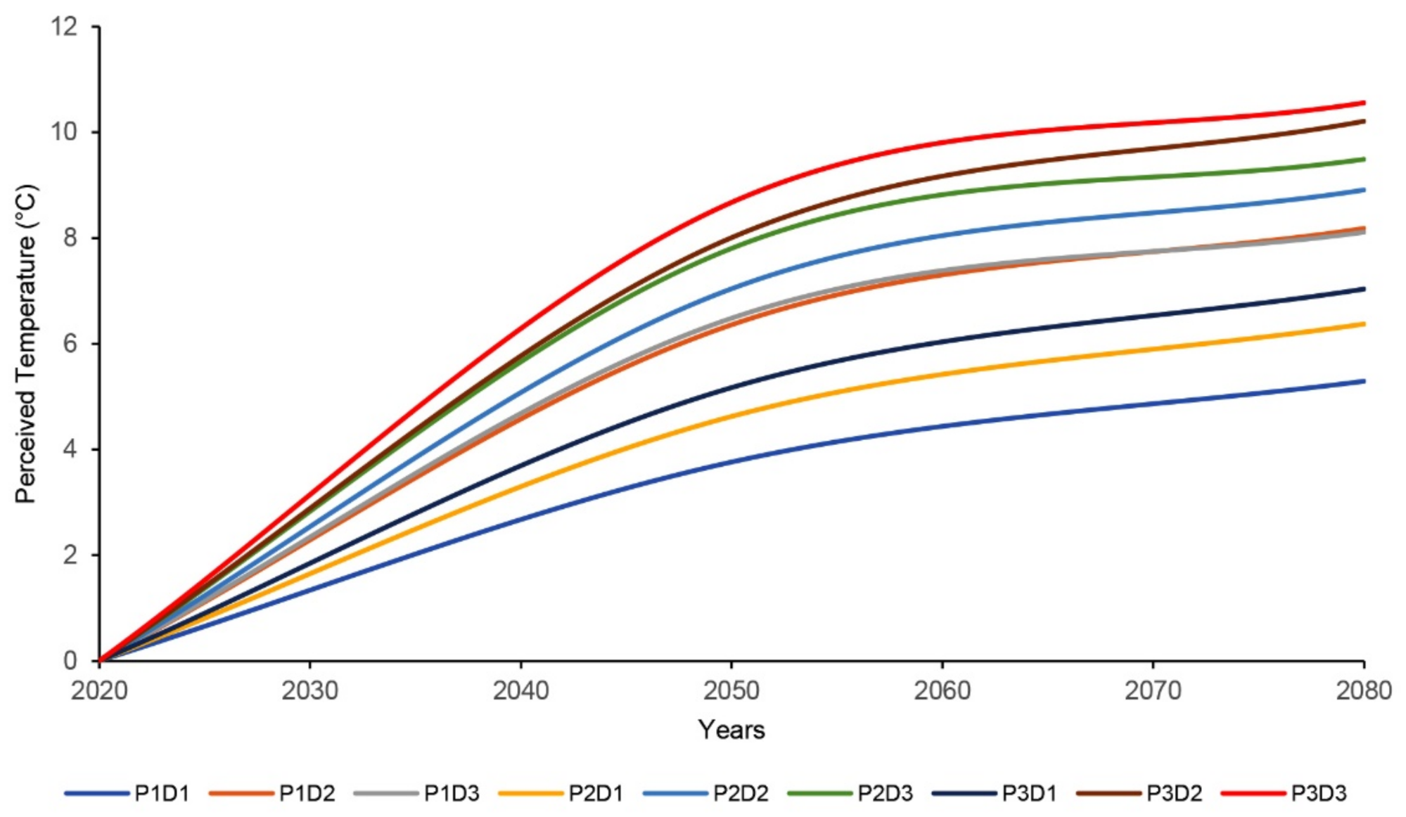
Accordingly, an accurate validation equation that presents the lowest RMSE value was taken from the first prediction’s equation in point 1 during the first day (15 July) (Table 9). It is necessary to refer that the PT index prediction’s algorithm is generated for specific boundary conditions: climate zone (BWh), summer period (July: extreme heat month), when the general weather boundaries are limited between minimum and maximum of air temperature among 0 and 50 °C, and humidity among 5% and 70%, respectively. Moreover, the typical housing neighborhood (multifamily housing) provides a close hourly/yearly prediction of the PT index in the study area (Figure 8).

5. Discussion

In this study, the outdoor thermal comfort variations inside multifamily housing neighborhoods in Saharan lands of Algeria and their long-term predictions were investigated on the basis of the TMY datasets and IPCC future scenarios. With the support of numerical simulations supported by ENVI-met software and thermal calculations under RayMan model, a new mathematic algorithm reliable for future patterns of outdoor thermal comfort in arid regions across Algerian oases territories was generated. The following discussion presents the key study findings, describes the study’s strengths and limitations explains the implications for the practice and suggests future research.

5.1. Findings and Recommendations

The study shows a gradual increase in PT index values, beginning from 2020 and progressively elevated to 2080 during the hot season, and refers to an extreme thermal heat stress level. The difference in PT index averages at the hot season between 2020 and 2050 was (+5.9 °C), and 2080 (+7.7 °C), which means a change from the slightly warm thermal stress zone to warm and hot thermal stress zones, respectively, due notably to the predicted climate change according to (AR4).

Surprisingly, no comfortable thermal stress zone was found during the 2080 period. However, only one comfortable hour was found at 2050 within two points, namely 02 and 03. On the other hand, the comfortable thermal zone represented 25% of the daily thermal stress level during the hot season in 2020. The thermal stress elevation is likely due to climate changes and their significant impact on arid lands.

As expected, climate change has an important effect on thermal stress through outdoor places without shading arrangements or spaces with significant SVF degrees. Most unfavorable places are exposed for a long time to the sun. Otherwise, multifamily housing represents a vulnerable urban form against climate changes in the long-term. Interestingly, the highest increase in future thermal heat stress was found by the A1B scenario characterized by rapid demography and a balance on the energy sources use. This increase has occurred inside different spatial configurations of the multifamily housing categories. Moreover, in the summer season, the hot thermal stress zone is enlarged during the day, from 8:00 a.m. to midnight, while the very hot thermal stress zone is more enlarged during the daytime hours, for 9 h, from between 9:00 a.m. to 6:00 p.m.

Otherwise, no very hot thermal stress zone was shown in the first period of 2020, whereas the hot thermal stress zone presented 5 h in the daytime, from 12:00 p.m. to 5:00 p.m. It is also interesting to develop a greedy algorithm for the PT thermal index predictions, typically for the multifamily housing sector, whereas the outputs related to the algorithm are required hourly/yearly values at the same time.

5.2. Strength and Limitations

The strength of this study is firmly due to its crossover of empirical and numerical approaches to quantify the outdoor thermal comfort within an oasis territory in the arid lands. Furthermore, the current study provides new findings of outdoor thermal comfort predictions in the arid climate, basically on long-term evaluation within current and future climate change scenarios.

None of the previous studies has investigated the predictions of outdoor thermal comfort or long-term weather patterns, specifically inside the oases settlements in arid climate, using TMY and (AR4) datasets. Consequentially, the study outcomes are considered key findings for outdoor thermal comfort predictions and redevelop them to cover all climate zones in the country. The findings are related to the study context but could be strongly enlarged by following the same methods and approaches for different climate and urban forms.

Long-term overheating in arid lands is unsafe to the human body and significantly impacts residents’ well-being, satisfaction and productivity. Despite climate change and the continuous heatwaves, human health in oases settlements can be critical and reveals a subject of rising in morbidity and mortality rates.

The evaluation of the human heat budget by monitoring and modeling urban thermal comfort during extreme weather conditions in the summer was an essential objective of the current study. Further, results can be used to assess the impact of thermal discomfort increases on the oases settlements’ livelihood, tourism activities and health situations. The outcomes illustrate the big necessity of developing a set of urban design procedures and policies to be integrated with arid lands for the long-term.

The algorithm allows numerical software used for urban climate studies in several thermal stress scenarios based on the PT index for short- and long-term patterns. Thus, it is necessary to indicate that the generated algorithm is mathematically able to be applied in different software’s databases, such as ENVI-met, Grasshopper and EnergyPlus.

Otherwise, our research has few limitations. The most significant limitation is the use of one urban housing typology. Even though the used multifamily housing archetype represents Algeria’s major household typologies, single-family households represent a considerable part of the residential building stock. Moreover, the study focused only on the hot period. The monitoring for an extended period (one year or more) may assist in assessing the thermal comfort changes throughout the year and predict the heat stress in all seasons. The predictions are limited only to one climate zone (BWh), one geographical context (Tolga Oases Complex, Biskra province) or a similar area, which means that the generated algorithm cannot be applied for other climate zones, as well as different regions. However, it could be more valuable to utilize the Fifth Assessment Report (AR5) anomalies of IPCC reports based on RCPs rather than SRES set of the Fourth Assessment Report (AR4) to provide more relevant future predictions. It is still limited in Meteonorm 7.2, the only available weather generator tool for our study.

On the other hand, for further development of a generated algorithm, it will be more reliable to perform a complete probabilistic treatment for the algorithm’s stability. In our case, we validated the algorithm-developed data merely based on RMSE.

It is necessary to indicate that building materials’ characteristics are mandatory for the assessment of the thermal fluctuations, specifically through the building scale. In our case study, it should be taken into consideration the thermal efficiency of building materials, such as the hollow bricks; their orientation; porosity; and the heat capacity to have their impact on thermal comfort [69,70]. However, our numerical modeling on ENVI-met software is very close to the existent investigated area, endowed with all the neighborhood’s constructive characteristics.

5.3. Implication on Practice and Research

This study allows urban climate researchers, architects, designers and urban planners several insights into predicted climate circumstances and their impacts on outdoor thermal comfort for the long-term under extreme weather conditions. Furthermore, the predicted results should be considered according to the large value on thermal stress changes within the following years. Natural ventilation or increasing the airflow, and improving outdoor shading are essential in the oasis urban fabric. Thermal predictions allow future designers to react to climate change better and think the best fit for climate adaptations, strategies and solutions to design and implement comfortable and efficient urban planning designs.

We believe that numerous solutions attempt for heat stress reduction and cooling energy savings were developed through the worldwide arid regions, such as the incorporation of PCMs in the built environment, especially among the residential sector [71,72]. This method can reduce the indoor temperature during the summer months by up to 2.04 °C and cooling energy savings up to 40.43 kWh [73], which could be beneficial for the external spaces as well. Hence, the utilization of PCM must be supported by dense external shading to benefit from the outdoor thermal heat stress balance and the cooling energy savings as well [74]. In this case, for future urban projects, the buildings’ orientation is crucial, and representative buildings’ shells composition should be chosen to reach the optimum PCM [72].

The human thermal indices need to be improved and applied in microclimatic predictions. This study highlights the biometeorological studies to promote a new process of outdoor thermal comfort long-term predictions among the worldwide climate zones and inside different urban contexts.

The Algerian government, especially the Ministry of Urban Planning and Housing, as well as the Ministry of Environment, may do an in-depth review regarding the built environment and the future strategies in urban housing against extreme weather conditions changing, notably in the arid lands, which became more and more vulnerable during the time. Additionally, we believe that not only architects or urban experts should be concerned with this study, but also climate scientists, especially in the meteorological field. We can enormously benefit from our key findings to see beyond the climate change impacts and predict the short and long-term conditions.

6. Conclusions

In this study, the predictions of the outdoor thermal comfort through an urban housing archetype in the Tolga Oases Complex were investigated during different weather conditions (TMY) and (AR4) scenarios. These were used to understand better predicting the impact of urban housing archetypes on the outdoor thermal comfort in an arid climate for the long-term. The researchers analyzed the evolution of the heat stress levels in the middle of an urban housing neighborhood which is representative of the most urban residential typology in Algeria. The outdoor thermal comfort assessment was performed over a long-term period (60 years) and basically by using the PT thermal index. According to the results, climate change has a significant impact on the outdoor thermal quality for upcoming years, and PT index values show a high elevation on heat stress during the hot season when the comfortable thermal zone is decreasing from 25% in 2020 to 1% in 2050 and 0% in 2080. The study suite was the generation of an algorithm for the PT index predictions in the short-term, medium-term and long-term future under extreme conditions related to the investigated climate zone, urban housing archetype and the conducted period. Accordingly, the algorithm could be enlarged to cover several climate zones during all seasons and multi-urban forms. This paper aimed to evaluate the impact of future long-term weather conditions on outdoor thermal comfort within a multifamily residential neighborhood. Future work should be performed by using different climate zones in Algeria during all the seasons to assess the thermal comfort fluctuations covering major cities in all the country over the year.

Our research further reflects that proper weather datasets based on reliable data from climate models and future emissions scenarios are required to help urban planners and architects to check their design solutions under future climate forecasting, especially in the arid climate. Furthermore, the outcomes present guidelines for landscape and urban designers who want to design thermally comfortable outdoor environments for these specific lands. Moreover, our findings suggest that architects, urban planners and climatologists should take into account the climate-change effects in the long-term concerning urban growth. In addition, the urban strategies should involve an urban model adapted to oases territories, proper to a sustainable green area and arid climate, and moderating the potential increase in air humidity.

References

- Roshan, G.; Moghbel, M.; Attia, S. Evaluating the wind cooling potential on outdoor thermal comfort in selected Iranian climate types. J. Therm. Biol. 2020, 92, 102660. [Google Scholar] [CrossRef]
- Jamei, E.; Rajagopalan, P.; Seyedmahmoudian, M.; Jamei, Y. Review on the impact of urban geometry and pedestrian level greening on outdoor thermal comfort. Renew. Sustain. Energy Rev. 2016, 54, 1002–1017. [Google Scholar] [CrossRef]
- Roshan, G.; Almomenin, H.S.; da Silveira Hirashima, S.Q.; Attia, S. Estimate of outdoor thermal comfort zones for different climatic regions of Iran. Urban Clim. 2019, 27, 8–23. [Google Scholar] [CrossRef]
- Attia, S. Spatial and Behavioral Thermal Adaptation in Net Zero Energy Buildings: An Exploratory Investigation. Sustainability 2020, 12, 7961. [Google Scholar] [CrossRef]
- Attia, S.; Levinson, R.; Ndongo, E.; Holzer, P.; Kazanci, O.B.; Homaei, S.; Zhang, C.; Olesen, B.W.; Qi, D.; Hamdy, M.; et al. Resilient cooling of buildings to protect against heat waves and power outages: Key concepts and definition. Energy Build. 2021, 239, 110869. [Google Scholar] [CrossRef]
- Elnabawi, M.H.; Hamza, N. Behavioural perspectives of outdoor thermal comfort in urban areas: A critical review. Atmosphere 2020, 11, 51. [Google Scholar] [CrossRef] [Green Version]
- Nakicenovic, N.; Alcamo, J.; Davis, G.; Vries, B.D.; Fenhann, J.; Gaffin, S.; Gregory, K.; Grübler, A.; Jong, T.Y.; Kram, T.; et al. Special Report on Emissions Scenarios; Cambridge University Press: Cambridge, UK, 2000. [Google Scholar]
- Moazami, A.; Nik, V.M.; Carlucci, S.; Geving, S. Impacts of future weather data typology on building energy performance–Investigating long-term patterns of climate change and extreme weather conditions. Appl. Energy 2019, 238, 696–720. [Google Scholar] [CrossRef]
- Hamstead, Z.A.; Iwaniec, D.M.; McPhearson, T.; Berbés-Blázquez, M.; Cook, E.M.; Muñoz-Erickson, T.A. Resilient Urban Futures. 2021. Available online: https://0-www-springer-com.brum.beds.ac.uk/gp/book/9783030631307 (accessed on 13 March 2021).
- Coccolo, S.; Kämpf, J.; Scartezzini, J.L.; Pearlmutter, D. Outdoor human comfort and thermal stress: A comprehensive review on models and standards. Urban. Clim. 2016, 18, 33–57. [Google Scholar] [CrossRef]
- Palme, M.; Salvati, A. Urban Microclimate Modelling for Comfort and Energy Studies; Springer International Publishing: Berlin/Heidelberg, Germany, 2021. [Google Scholar]
- Kenawy, I.; Lam, C.K.C.; Shooshtarian, S. Summer outdoor thermal benchmarks in Melbourne: Applications of different techniques. Build. Environ. 2021, 195, 107658. [Google Scholar] [CrossRef]
- Moazami, A.; Carlucci, S.; Causone, F.; Pagliano, L. Energy retrofit of a day care center for current and future weather scenarios. Procedia Eng. 2016, 145, 1330–1337. [Google Scholar] [CrossRef] [Green Version]
- Tootkaboni, M.P.; Ballarini, I.; Zinzi, M.; Corrado, V. A Comparative Analysis of Different Future Weather Data for Building Energy Performance Simulation. Climate 2021, 9, 37. [Google Scholar] [CrossRef]
- Nematchoua, M.K.; Yvon, A.; Kalameu, O.; Asadi, S.; Choudhary, R.; Reiter, S. Impact of climate change on demands for heating and cooling energy in hospitals: An in-depth case study of six islands located in the Indian Ocean region. Sustain. Cities Soc. 2019, 44, 629–645. [Google Scholar] [CrossRef]
- Yau, Y.H.; Hasbi, S. A review of climate change impacts on commercial buildings and their technical services in the tropics. Renew. Sustain. Energy Rev. 2013, 18, 430–441. [Google Scholar] [CrossRef]
- de Wilde, P.; Coley, D. The implications of a changing climate for buildings. Build. Environ. 2012, 55, 1–7. [Google Scholar] [CrossRef] [Green Version]
- Berger, T.; Amann, C.; Formayer, H.; Korjenic, A.; Pospischal, B.; Neururer, C.; Smutny, R. Impacts of climate change upon cooling and heating energy demand of office buildings in Vienna, Austria. Energy Build. 2014, 80, 517–530. [Google Scholar] [CrossRef]
- Guan, L. Preparation of future weather data to study the impact of climate change on buildings. Build. Environ. 2009, 44, 793–800. [Google Scholar] [CrossRef]
- Roetzel, A.; Tsangrassoulis, A. Impact of climate change on comfort and energy performance in offices. Build. Environ. 2012, 57, 349–361. [Google Scholar] [CrossRef]
- Nicol, J.F.; Humphreys, M.A. Adaptive thermal comfort and sustainable thermal standards for buildings. Energy Build. 2002, 34, 563–572. [Google Scholar] [CrossRef]
- Bughio, M.; Schuetze, T.; Mahar, W.A. Comparative Analysis of Indoor Environmental Quality of Architectural Campus Buildings’ Lecture Halls and its Perception by Building Users in Karachi, Pakistan. Sustainability 2020, 12, 2995. [Google Scholar] [CrossRef] [Green Version]
- Mahar, W.A. Methodology for the Design of Climate-Responsive Houses for Improved Thermal Comfort in Cold Semi-Arid Climates. Ph.D. Thesis, University of Liège, Liege, Belgium, 2021. [Google Scholar]
- Mahar, W.A.; Amer, M.; Attia, S. Indoor thermal comfort assessment of residential building stock in Quetta, Pakistan. In Proceedings of the European Network for Housing Research (ENHR) Annual Conference 2018, Uppsala, Sweden, 27–29 June 2018; Available online: https://orbi.uliege.be/handle/2268/226537 (accessed on 13 March 2021).
- De Freitas, C.R.; Grigorieva, E.A. A comprehensive catalogue and classification of human thermal climate indices. Int. J. Biometeorol. 2015, 59, 109–120. [Google Scholar] [CrossRef]
- De Freitas, C.R.; Grigorieva, E.A. A comparison and appraisal of a comprehensive range of human thermal climate indices. Int. J. Biometeorol. 2017, 61, 487–512. [Google Scholar] [CrossRef] [PubMed]
- Budd, G.M. Wet-bulb globe temperature (WBGT)—Its history and its limitations. J. Sci. Med. Sport 2008, 11, 20–32. [Google Scholar] [CrossRef]
- Thom, E.C. The discomfort index. Weatherwise 1959, 12, 57–61. [Google Scholar] [CrossRef]
- Höppe, P. The physiological equivalent temperature–a universal index for the biometeorological assessment of the thermal environment. Int. J. Biometeorol. 1999, 43, 71–75. [Google Scholar] [CrossRef]
- Staiger, H.; Laschewski, G.; Grätz, A. The perceived temperature–a versatile index for the assessment of the human thermal environment. Part. A Sci. Basics. Int. J. Biometeorol. 2012, 56, 165–176. [Google Scholar] [CrossRef] [PubMed]
- Staiger, H.; Laschewski, G.; Matzarakis, A. Selection of appropriate thermal indices for applications in human biometeorological studies. Atmosphere 2019, 10, 18. [Google Scholar] [CrossRef] [Green Version]
- Jendritzky, G.; Staiger, H.; Bucher, K.; Graetz, A.; Laschewski, G. The Perceived Temperature: The Method of the Deutscher Wetterdienst for the Assessment of Cold Stress and Heat Load for the Human Body. Internet Workshop on Windchill, Hosted by Environment Canada; 3–7 April 2000. Available online: https://www.semanticscholar.org/paper/The-Perceived-Temperature-%3A-The-Method-of-the-for-Jendritzky-Staiger/f62308d669ed828021e90450c002f4e89d5355cd (accessed on 15 March 2021).
- Matzarakis, A.; Rutz, F.; Mayer, H. Modelling radiation fluxes in simple and complex environments—Application of the RayMan model. Int. J. Biometeorol. 2007, 51, 323–334. [Google Scholar] [CrossRef]
- Matzarakis, A.; Rutz, F.; Mayer, H. Modelling radiation fluxes in simple and complex environments: Basics of the RayMan model. Int. J. Biometeorol. 2010, 54, 131–139. [Google Scholar] [CrossRef] [Green Version]
- Jendritzky, G.; Nübler, W. A model analysing the urban thermal environment in physiologically significant terms. Arch. Meteorol. Geophys. Bioclimatol. Ser. B 1981, 29, 313–326. [Google Scholar] [CrossRef]
- Jendritzky, G. Perceived Temperature: Klima-Michel-Model, The Development of Heat Stress Watch Warning Systems. Health and Global Environment Change, Heat-waves: Risks and responses. Freiburg 2003, 2, 39. [Google Scholar]
- Gosling, S.; Bryce, E.K.; Dixon, P.G.; Gabriel, K.; Gosling, E.Y.; Hanes, J.M.; Hondula, D.M.; Liang, L.; Mac Lean, P.A.B.; Muthers, S.; et al. A glossary for biometeorology. Int. J. Biometeorol. 2014, 58, 277–308. [Google Scholar] [CrossRef]
- Byon, J.Y.; Kim, J.S.; Kim, J.Y.; Choi, B.C.; Choi, Y.J.; Graetz, A. A study on the characteristics of perceived temperature over the Korean peninsula during 2007 summer. Atmosphere 2008, 18, 137–146. [Google Scholar]
- Lee, D.G.; Byon, J.Y.; Choi, Y.J.; Kim, K.R. Relationship between summer heat stress (perceived temperature) and daily excess mortality in Seoul during 1991~2005. J. Korean Soc. Atmos. Environ. 2010, 26, 253–264. [Google Scholar] [CrossRef] [Green Version]
- Wang, S.; Zhu, J. Amplified or exaggerated changes in perceived temperature extremes under global warming. Clim. Dyn. 2020, 54, 117–127. [Google Scholar] [CrossRef]
- Fang, Z.; Zheng, Z.; Feng, X.; Shi, D.; Lin, Z.; Gao, Y. Investigation of outdoor thermal comfort prediction models in South China: A case study in Guangzhou. Build. Environ. 2021, 188, 107424. [Google Scholar] [CrossRef]
- Cheung, C.S.C.; Hart, M.A. Climate change and thermal comfort in Hong Kong. Int. J. Biometeorol. 2014, 58, 137–148. [Google Scholar] [CrossRef] [PubMed]
- Liu, S.; Pan, W.; Zhao, X.; Zhang, H.; Cheng, X.; Long, Z.; Chen, Q. Influence of surrounding buildings on wind flow around a building predicted by CFD simulations. Build. Environ. 2018, 140, 1–10. [Google Scholar] [CrossRef]
- Nazarian, N.; Fan, J.; Sin, T.; Norford, L.; Kleissl, J. Predicting outdoor thermal comfort in urban environments: A 3D numerical model for standard effective temperature. Urban. Clim. 2017, 20, 251–267. [Google Scholar] [CrossRef]
- Kariminia, S.; Ahmad, S.S.; Omar, M.; Ibrahim, N. Urban outdoor thermal comfort prediction for public square in moderate and dry climate. In Proceedings of the 2011 IEEE Symposium on Business, Engineering and Industrial Applications (ISBEIA), Langkawi, Malaysia, 25–28 September 2011; pp. 308–313. [Google Scholar]
- Semahi, S.; Benbouras, M.A.; Mahar, W.A.; Zemmouri, N.; Attia, S. Development of Spatial Distribution Maps for Energy Demand and Thermal Comfort Estimation in Algeria. Sustainability 2020, 12, 6066. [Google Scholar] [CrossRef]
- Lee, H. Intergovernmental Panel on Climate Change; World Merteorological Organization: Geneva, Switzerland, 2007; Available online: https://0-www-mdpi-com.brum.beds.ac.uk/journal/energies/special_issues/Social_Fuel_Cell (accessed on 13 March 2021).
- Houghton, E. Climate Change 1995: The Science of Climate Change: Contribution of Working Group I to the Second Assessment Report of the Intergovernmental Panel on Climate Change; Cambridge University Press: Cambridge, UK, 1996; Volume 2. [Google Scholar]
- Bernstein, L.; Bosch, P.; Canziani, O.; Chen, Z.; Christ, R.; Davidson, O.; Hare, W.; Huq, S.; Karoly, D.; Kattsov, V.; et al. Climate Change 2007 Synthesis Report; Intergovernmental Panel on Climate Change: Geneva, Switzerland, 2008. [Google Scholar]
- Bughio, M.; Khan, M.S.; Mahar, W.A.; Schuetze, T. Impact of passive energy efficiency measures on cooling energy demand in an architectural campus building in Karachi, Pakistan. Sustainability 2021, 13, 7251. [Google Scholar] [CrossRef]
- Mahar, W.A.; Verbeeck GReiter, S.; Attia, S. Sensitivity analysis of passive design strategies for residential buildings in cold semi-arid climates. Sustainability 2020, 12, 1091. [Google Scholar] [CrossRef] [Green Version]
- Remund, J.; Müller, S.C.; Schilter, C.; Rihm, B. The use of Meteonorm weather generator for climate change studies. In Proceedings of the 10th EMS Annual Meeting Abstracts, Zürich, Switzerland, 13–17 September 2010; Volume 7, p. EMS2010-417. [Google Scholar]
- Crawley, D.B.; Lawrie, L.K. Rethinking the TMY: Is the ‘typical’meteorological year best for building performance simulation? In Proceedings of the 14th Conference of International Building Performance Simulation Association BS2015, Hyderabad, India, 7–9 December 2015; pp. 2655–2662. [Google Scholar]
- Richter, M. Urban climate change-related effects on extreme heat events in Rostock, Germany. Urban Ecosyst. 2016, 19, 849–866. [Google Scholar] [CrossRef]
- Carter, J.G. Urban climate change adaptation: Exploring the implications of future land cover scenarios. Cities 2018, 77, 73–80. [Google Scholar] [CrossRef] [Green Version]
- Semahi, S.; Zemmouri, N.; Singh, M.K.; Attia, S. Comparative bioclimatic approach for comfort and passive heating and cooling strategies in Algeria. Build. Environ. 2019, 161, 106271. [Google Scholar] [CrossRef] [Green Version]
- Matallah, M.E.; Alkama, D.; Ahriz, A.; Attia, S. Assessment of the Outdoor Thermal Comfort in Oases Settlements. Atmosphere 2020, 11, 185. [Google Scholar] [CrossRef] [Green Version]
- Labdaoui, K.; Mazouz, S.; Acidi, A.; Cools, M.; Moeinaddini, M.; Teller, J. Utilising thermal comfort and walking facilities to propose a comfort walkability index (CWI) at the neighbourhood level. Build. Environ. 2021, 193, 107627. [Google Scholar] [CrossRef]
- Engl. VDI/DIN-Kommission Reinhaltung der Luft (KRdL)-Normenausschuss. 3787, Part 2: Environmental meteorology, methods for the human-biometeorological evaluation of climate and air quality for the urban and regional planning at regional level. Part I: Climate. VDI/DIN-Handb. Reinhalt. Luft. 2008, 1, 1–32. [Google Scholar]
- Meteonorm Software. Available online: https://meteonorm.com/en/ (accessed on 15 March 2021).
- Matallah, M.E.; Alkama, D.; Teller, J.; Ahriz, A.; Attia, S. Quantification of the Outdoor Thermal Comfort within Different Oases Urban Fabrics. Sustainability 2021, 13, 3051. [Google Scholar] [CrossRef]
- ENVI-Met Software. 2020. Available online: https://www.envi-met.com/ (accessed on 10 October 2020).
- Bruse, M.; Fleer, H. Simulating surface–plant–air interactions inside urban environments with a three dimensional numerical model. Environ. Model. Softw. 1998, 13, 373–384. [Google Scholar] [CrossRef]
- Bruse, M. ENVI-Met. 3.0: Updated Model. Overview; University of Bochum: Bochum, Germany; Available online: www.envi-met.com (accessed on 15 June 2004).
- ASHRAE. ASHRAE Guideline 14–2014, Measurement of Energy, Demand, and Water Savings; ASHRAE: Atlanta, GA, USA, 2014. [Google Scholar]
- Matallah, M.E.; Ahriz, A.; Attia, S. Quantification of the Outdoor Thermal Comfort Process: Simulation & Calculation Data (No. 01/2020); Sustainable Building Design Lab; University of Liège: Liège, Belgium, 2020; Available online: http://hdl.handle.net/2268/250205 (accessed on 15 March 2021).
- Vince, A. A framework for the greedy algorithm. Discret. Appl. Math. 2002, 121, 247–260. [Google Scholar] [CrossRef] [Green Version]
- Edmonds, J. Matroids and the greedy algorithm. Math. Program. 1971, 1, 127–136. [Google Scholar] [CrossRef]
- Pavlík, Z.; Jerman, M.; Fořt, J.; Černý, R. Monitoring thermal performance of hollow bricks with different cavity fillers in difference climate conditions. Int. J. Thermophys. 2015, 36, 557–568. [Google Scholar] [CrossRef]
- Pavlík, Z.; Jerman, M.; Trník, A.; Kočí, V.; Černý, R. Effective thermal conductivity of hollow bricks with cavities filled by air and expanded polystyrene. J. Build. Phys. 2014, 37, 436–448. [Google Scholar] [CrossRef]
- Sovetova, M.; Memon, S.A.; Kim, J. Thermal performance and energy efficiency of building integrated with PCMs in hot desert climate region. Sol. Energy 2019, 189, 357–371. [Google Scholar] [CrossRef]
- Wahid, M.A.; Hosseini, S.E.; Hussen, H.M.; Akeiber, H.J.; Saud, S.N.; Mohammad, A.T. An overview of phase change materials for construction architecture thermal management in hot and dry climate region. Appl. Therm. Eng. 2017, 112, 1240–1259. [Google Scholar] [CrossRef]
- Memon, S.A. Phase change materials integrated in building walls: A state of the art review. Renew. Sustain. Energy Rev. 2014, 31, 870–906. [Google Scholar] [CrossRef]
- Nematchoua, M.K.; Noelson, J.C.V.; Saadi, I.; Kenfack, H.; Andrianaharinjaka, A.Z.F.; Ngoumdoum, D.F.; Sela, J.B.; Reiter, S. Application of phase change materials, thermal insulation, and external shading for thermal comfort improvement and cooling energy demand reduction in an office building under different coastal tropical climates. Sol. Energy 2020, 207, 458–470. [Google Scholar] [CrossRef]
Figure 1.
Conceptual study framework.
Figure 2.
Location of the study area: (a) Biskra Province, (b) Tolga Oases Complex and (c) Tolga city.
Figure 3.
The multifamily housing neighborhood building’s shapes and configuration.
Figure 4.
PT index values evolution during all the studied periods.
Figure 5.
PT index averages’ differences from 2020 to 2080.
Figure 6.
Workflow steps of the PT thermal index predictions algorithm.
Figure 7.
PT index averages’ variations during three days among: 2020, 2050 and 2080 in point 1: (a) 15 July, (b) 16 July, and (c) 17 July.
Figure 8.
A framework of PT index predictions algorithm from inputs to outputs.