Application of Meteorological Variables for the Estimation of Static Load Model Parameters

Abstract

This paper presents a novel approach for estimating the parameters of the most frequently used static load model, which is based on the use of meteorological variables and is an alternative to the commonly used but time-consuming measurement-based approach. The presented model employs five frequently reported meteorological variables (ambient temperature, relative humidity, atmospheric pressure, wind speed, and wind direction) and the load model parameters as the independent and dependent variables, respectively. The analysis compared the load model parameters obtained by using all five meteorological variables and also when the meteorological variables with the lowest influence are omitted successively (one by one) from the model. It is recommended based on these results to use the model with the maximum accuracy, i.e., with five meteorological variables. The model was validated on a validation set of measurements, demonstrating its applicability for the estimation of load model parameters when the measurements of electrical variables for parameter identification are not available. Finally, load model parameters of the analyzed demand were estimated on the basis of only ambient temperature, and it was found that such a linear model can be used with a similar accuracy as the models with up to four meteorological variables.

1. Introduction

Accurate modeling of supplied load is very important for the analysis of power supply systems. Amongst the numerous static and dynamic load models [1], the most frequently used load model in both steady state and dynamic power system studies is the exponential static load model [2]. Generally, load models are identified by using component-based approaches, measurement-based approaches, or a combination of these two [3,4]. In the case of component-based approaches, load composition and models of individual load devices are input data; for measurement-based approaches, field measurement data are required.

During the last decade, measurement-based load modeling approaches have become prevalent, as the characteristics of different field monitoring equipment became improved and their costs are reduced. Field monitoring equipment can record voltage changes and consequent changes in power demands, which then can be used for the determination of load model parameters; recent improvements of recording devices include significant internal memory, enabling users to perform long time measurements of relevant electric variables [5]. The older monitoring equipment that was already installed can also be used to record data that can be applied for the identification of load model parameters [6,7].

Many procedures for the measurement-based identification of load model parameters are previously developed, e.g., [8,9,10]. Typically, the implemented procedures for the identification of the load model parameters use data on transient voltage changes and subsequent active and reactive power responses recorded during normal operating conditions [5,9,10,11,12], or in specifically designed field experiments [13,14]. Most of the previous work deal with the determination of load model parameters in high and medium voltage networks, while the results of identification of load model parameters in low voltage (LV) networks are presented in a relatively small number of references. The main reason is the strong influence of stochastic load changes on power responses to voltage changes in LV networks [5,15,16,17]. In order to obtain reliable load model parameters in LV networks, the measurements are performed over longer time periods, and results are presented using a statistical analysis of the load model parameters. For example, the authors in [5] and in [16] provided the load model parameters of one LV bus obtained for one season and for the whole year, respectively.

The comprehensive research on load model parameters of LV-connected administrative buildings is presented in [17], where statistically processed parameters of static exponential load model for administrative class of customers are presented on the basis of measurements at different LV buses, in different seasons, on characteristic days of the week, and for specific periods of considered days. Furthermore, polynomial fitting functions that represent temporal changes of load model parameters during the characteristic days of the week are introduced.

This paper is the continuation of the research in [17], but it differs from that research and all previous work because it deals with the estimation of load model parameters by using nonelectrical variables, i.e., it uses meteorological variables commonly included in weather reports. As presented in [18], meteorological variables can be used for the estimation of monthly and annual electricity consumption, e.g., during specific months and for the whole year, but the main hypothesis in this paper is that meteorological variables can also be applied for the estimation of load model parameters for much shorter periods: days of the week and days in different seasons. The paper compares the results of parameter estimation of the selected static load model when one to five meteorological variables were used, in descending order from the largest number. On the basis of these comparisons and of a validation of parameter estimation, the paper recommends the model that provides the most accurate results. Furthermore, load model parameter estimation by using only ambient temperature, as the most common meteorological variable available in all weather reports, is presented and validated.

The structure of the rest of this paper is as follows: Section 2 introduces a procedure for an estimation of the parameters of a static exponential load model using different numbers of meteorological variables. Section 3 presents the results of the procedure from Section 2, compares these results with the parameters of the same class of customers who were determined on the basis of electrical variables, discusses the accuracy of the results, suggests the best model for parameter estimation from the meteorological variable data, and tests the applicability of the model when electrical variables are not available. Section 3 also presents the results of load model parameter estimation and their validation when only ambient temperature is applied as the input variable, while Section 4 summarizes the main conclusions of the paper and gives some recommendations for the future work.

2. Description of the Applied Procedure

All previously published procedures for load model parameter determination use electrical variables as input data. Commonly, these variables are voltage, frequency, and active and reactive power, since load models are expressed as active and reactive power dependencies on both voltage and frequency [1,2,3,4,5,6]. However, in many studies (e.g., steady-state analyses), dependencies on frequency can be omitted because frequency deviations can be neglected in steady-state operation conditions. One such load model in which dependencies on frequency are neglected is the static exponential load model:

$$P=P_0{\left(\frac{U}{U_0}\right)}^{k_{pu}} ,$$

(1)

$$Q=Q_0{\left(\frac{U}{U_0}\right)}^{k_{qu}} .$$

(2)

In (1) and (2), P and Q are respectively the active and reactive power at voltage U; P₀ and Q₀ are respectively the active and reactive power at the initial voltage, U₀; while k_pu and k_qu are the voltage exponents of active and reactive power, respectively. The voltage exponents are unknown load model parameters that should be determined by using one of load modelling approaches.

The application of measurement-based approaches for the determination of static exponential load model parameters in [17] also validates the results of the statistical analysis, and these results are used for the verification of the new procedure for parameter estimation presented in this paper. The new procedure is based on the application of meteorological variables for the estimation of static load model parameters, acknowledging that weather conditions influence customer activities in administrative buildings and therefore influence the way how certain electrical devices are used by customers. The procedure assumes linear relationships (i.e., linear model) between the dependent (response) variables k_pu and k_qu, and the values of independent (explanatory) meteorological variables in the time period in which related electrical variables are measured. These relationships are expressed in the forms (3) and (4):

$$k_{pu}=a_{1}T+a_{2}H+a_3{A}_p+a_4{W}_s+a_5{W}_d ,$$

(3)

$$k_{qu}=b_{1}T+b_{2}H+b_3{A}_p+b_4{W}_s+b_5{W}_d ,$$

(4)

where a₁, a₂, …, a₅, b₁, b₂, …, b₅ are the parameters of the assumed relationships; T, H, A_p, W_s and W_d are ambient temperature (in °C), relative humidity (%), atmospheric pressure (mBar), wind speed (m/s), and wind direction, respectively. For the purpose of this paper, the wind direction is expressed in degree clockwise, where zero corresponds to the north direction. Wind direction is considered in model (3) and (4), since in examined geographical area it indicates specific changes in weather, i.e., changes of the warm weather into the cold, wet weather into the dry, and vice versa. All listed meteorological variables are applied because they are frequently available in weather reports. Their values are taken from [19] for considering the area of the town Leskovac (Republic of Serbia), where a measurement campaign of electrical variables was performed in order to determine reliable load model parameters. From the sets of values of meteorological variables, values corresponding to the hour in which a voltage change (used for load model parameter identification) occurred are identified and grouped with the corresponding k_pu and k_qu values. In that way, datasets of meteorological variable values and load model parameter values were formed, and a multiple linear regression [20,21,22,23] is performed to identify parameters a₁, a₂, …, a₅, b₁, b₂, …, b₅ of the model in (3) and (4).

In the case when some meteorological variables do not influence the results significantly, such variables can be omitted from the analysis, and simplified forms of linear relationships that do not include dependencies on these variables can be adopted. Since meteorological variables in (3) and (4) are expressed in different units and scales/ranges, the greater absolute value of the parameter does not necessarily denote the more significant influence on the dependent variable, and vice versa. To gain insight into the relative influence of independent variables on dependent ones, partial flexibility coefficients are calculated. Each partial flexibility coefficient is the multiplication of the parameter that is in front of the independent variable and the average value of the independent variable, divided by the average value of the dependent variable [20]. For example, the partial flexibility coefficient of relative humidity in (3) can be denoted as k_{pu_H} and calculated by this formula:

$$k_{pu\_H}=\frac{a_2{H}_{av}}{k_{pu\_av}} ,$$

(5)

where H_av and k_{pu_av} are the average values of H and k_pu, respectively.

Partial flexibility coefficients of different meteorological variables included in the model (3) and (4) are mutually compared separately for both models, and the variable with the smallest absolute value of partial flexibility coefficient is omitted from the model. Therefore, simplified relationships between independent variables k_pu and k_qu and meteorological variables—which are similar to (3) and (4), but with one or more terms deleted—are used in the next iteration of the procedure. The procedure continues until only one meteorological variable is left in the model. At the end, the best model is selected for k_pu and k_pu among the available five models with different numbers of meteorological variables, where the selection criterion is the highest accuracy of model results.

The existence of mutual correlations of the independent variables is also checked. For the identification of multicollinearity between meteorological variables, variance inflation factors (VIFs) are calculated for each pair of independent variables [20,21]. The variance inflation factor between two variables, X and Y, is calculated according to this formula

$$VI{F}_{XY}=\frac{1}{1-R_{XY}^2} ,$$

(6)

where R_XY is the correlation coefficient between variables X and Y. In this paper, the variance inflation factors, VIFs, are calculated for pairs of the following meteorological variables: ambient temperature, T; relative humidity, H; atmospheric pressure, A_p; wind speed, W_s; and wind direction, W_d. Variance inflation factors that are smaller than 4, and especially those close to 1, mean that there are no multicollinearities. The values greater than 4, especially those greater than 10, show that very strong multicollinearity exists. In the latter case, one of two independent variables that take part in the multicollinearity should be eliminated from the analysis, and the values of VIF should be examined again. In this paper, the independent variable (that take part in the multicollinearity) with a smaller absolute value of partial flexibility coefficient is eliminated, regardless of whether this partial flexibility coefficient is the smallest one of all partial flexibility coefficients or not.

The procedure for the identification of the variables that are included in the relationships between load model parameters and meteorological variables for a particular season can be summarized as follows:

• Set the iteration number, i, to one (i = 1), and assume the linear model with all five meteorological variables included in the general relationships (3) and (4).
• Multiple linear regressions are applied to datasets of average values of load model parameters and corresponding the average values of 5-i + 1 meteorological variables. The parameters of the linear model with 5-i + 1 independent variables are obtained.
• If the iteration number is less than 5 (i < 5), i.e., if the number of meteorological variables is greater than 1 (5-i + 1 > 1), go to Step 4. Otherwise, end the procedure.
• Variance inflation factors are calculated for each pair of independent variables included in the linear model from Step 2, as well as partial flexibility coefficients of all independent (meteorological) variables.
• If one variance inflation factor between two meteorological variables is greater than 4, partial flexibility coefficients of these variables are mutually compared; the variable with a smaller coefficient is then omitted from further analysis, and the procedure continues to Step 8. Otherwise, the procedure continues to Step 6.
• If two or more variance inflation factors between the meteorological variables are greater than 4, the variables with the greatest variance inflation factors are selected, and the partial flexibility coefficients of these variables are mutually compared. The variable with a smaller coefficient is omitted from further analysis, and the procedure continues to Step 8. Otherwise, the procedure continues to Step 7.
• Partial flexibility coefficients of all meteorological variables included in linear model from Step 2 are mutually compared, and the variable with smaller coefficient is omitted from further analysis.
• Increase the iteration number, i = i + 1, and go to Step 2.

3. Results

3.1. Analysis of Meteorological Variables during the Year

For the analysis of the influence of each meteorological variable on load model parameters during the year, datasets of the values of load model parameters and meteorological variables are firstly formed. They include the following: 1622 and 2002 identified k_pu and k_qu values, respectively, obtained from the “basic set of measurements” (see [17]) in different seasons, days of the week, and periods of the day; and the same numbers of corresponding values of meteorological variables.

As these datasets include the data during the year, the lower and upper bounds are specified for all considered meteorological variables. Thus, the temperature belongs to the range from −5 to 40 °C, the range of atmospheric pressure is from 995 to 1040 mBar, the upper and lower bounds of relative humidity are 18% and 100%, respectively, wind speed is in the range from 0 to 8 m/s, and wind direction belongs to the full range from 0° to 360°.

The analyses presented in the paper were performed separately for the winter, spring/autumn, and summer seasons. Average load model parameters were calculated in each 6 h time interval during three characteristic days, for every season. The same was performed for the meteorological variables. In that way, datasets of average values of load model parameters and meteorological variables were formed for winter, spring/autumn and summer.

3.2. Results of Multiple Linear Regression

In order to obtain relationships between the load model parameters of the examined demand of administrative buildings and five meteorological variables, at the beginning of the procedure (as described in Section 2) multiple linear regressions were applied to datasets of average values for different seasons. For example, the results (7) and (8) are obtained for winter:

$$k_{pu}=-0.11139T-0.03392H+0.00447A_p+0.3137W_s-4.173\times {10}^{-4}{W}_d ,$$

(7)

$$k_{qu}=0.08776T+0.03534H+9.0433\cdot {10}^{-4}{A}_p-0.89459W_s+0.00556W_d .$$

(8)

Table 1. VIFs between meteorological variables when k_pu and k_qu are calculated according to Equations (7) and (8).

VIFs	kpu					kqu
	T	H	Ap	Ws	Wd	T	H	Ap	Ws	Wd
T		6.290	7.132	1.057	1.137		4.813	5.033	1.019	1.001
H	6.290		77.174	1.110	1.181	4.813		72.925	1.008	1.006
Ap	7.132	77.174		1.059	1.230	5.033	72.925		1.021	1.013
Ws	1.057	1.110	1.059		1.103	1.019	1.008	1.021		1.598
Wd	1.137	1.181	1.230	1.103		1.001	1.006	1.013	1.598

presents the variance inflation factors between five meteorological variables applied for k_pu and k_qu estimations according to (7) and (8), while

Table 2. Partial flexibility coefficients of the meteorological variables included in linear relationships (7)–(14), (17)–(24), and (27)–(34).

Relationships	Meteorological Variable	Ambient Temperature, T	Relative Humidity, H	Atmospheric Pressure, Ap	Wind Speed, Ws	Wind Direction, Wd
(7) and (8)	(7)	−0.17859	−2.05823	3.14858	0.12386	0.03904
	(8)	−0.04073	0.00634	−3.01167	−0.00171	−0.00725
(9) and (10)	(9)	−0.03181	–	0.95091	0.05639	0.02468
	(10)	−0.00616	–	0.99392	−0.16851	0.18156
(11) and (12)	(11)	0.0314F7	–	0.96500	−0.06339	–
	(12)	–	–	0.98814	−0.16592	0.17676
(13) and (14)	(13)	−0.03447	–	1.03544	–	–
	(14)	–	–	0.92169	–	0.07845
(17) and (18)	(17)	−0.15977	−0.27691	1.54975	0.04606	−0.16183
	(18)	0.08436	0.26483	0.58218	−0.04528	0.11372
(19) and (20)	(19)	−0.06358	–	1.10271	0.06779	−0.10461
	(20)	−0.02109	–	0.97328	−0.03067	0.07918
(21) and (22)	(21)	–	–	1.08036	0.05327	−0.13473
	(22)	–	–	0.95836	−0.0287	0.06906
(23) and (24)	(23)	–	–	1.13997	–	−0.13672
	(24)	–	–	1.03896	−0.03882	–
(27) and (28)	(27)	−1.38144	−1.07968	4.935022	−0.00111	0.295455
	(28)	−0.0659847	−0.059010	0.50132	−0.01118	−0.00487
(29) and (30)	(29)	0.01654	–	1.01446	−0.02531	−0.00461
	(30)	−0.07827	–	0.91955	−0.00619	0.16367
(31) and (32)	(31)	0.01581	–	1.00684	−0.026	–
	(32)	–	–	0.84754	−0.02622	0.17933
(33) and (34)	(33)	–	–	1.02209	−0.02136	–
	(34)	–	–	0.85584	–	0.14470

lists the partial flexibility coefficients obtained in four iterations of the proposed procedure for an identification of the variables that are included in the relationships, for every season. The comparison of values from Table 1 confirms that very strong multicollinearity between humidity and atmospheric pressure exists, and one of these meteorological variables should be eliminated from the model. In considering that the partial flexibility coefficients of these variables relate to (7) and (8), it is thus reasoned that H and A_p should be omitted from the model of k_pu and k_qu, respectively. After these assumptions are adopted, (9) and (10) are obtained:

$$k_{pu}=-0.01984T+0.00135A_p+0.14281W_s+2.638\times {10}^{-4}{W}_d ,$$

(9)

$$k_{qu}=0.09035T+0.03628H-0.89194W_s+0.00557W_d .$$

(10)

According to the values of partial flexibility coefficients from Table 2 that relate meteorological variables included in (9) and (10), in the next iteration of the procedure, the wind direction and ambient temperature are omitted from the linear regression model of k_pu and k_qu, respectively, and (11) and (12) are obtained:

$$k_{pu}=-0.01963T+0.00137A_p+0.16053W_s ,$$

(11)

$$k_{qu}=0.03612H-0.91973W_s+0.0076W_d .$$

(12)

Further, W_s is eliminated from k_pu and k_qu model. For k_pu, VIF_{Ap_Ws} is found to be large, but the partial flexibility coefficient of W_s is smaller than the partial flexibility coefficient of A_p, and W_s is omitted in further analysis:

$$k_{pu}=-0.0215T+0.00147A_p ,$$

(13)

$$k_{qu}=0.03366H+0.00466W_d .$$

(14)

In the final iteration of the suggested procedure, T and W_d are eliminated from linear regression model of k_pu and k_qu, respectively:

$$k_{pu}=0.00142A_p ,$$

(15)

$$k_{qu}=0.03996H .$$

(16)

Thus, the simplest model (15) and (16) represent the dependencies of k_pu and k_qu on atmospheric pressure and relative humidity, respectively.

The relationships (7), (9), (11), (13), and (15), which express dependencies of k_pu on meteorological variables, are obtained with correlation coefficients, R [22,23], i.e., 0.998, 0.996, 0996, 0.996, and 0.995, respectively. These values indicate that there are strong correlations between k_pu and the meteorological variables in winter season. Similarly, the correlation coefficients of k_qu dependencies (8), (10), (12), (14), and (16) are 0.997, 0.997, 0.994, 0.993, and 0.990, i.e., k_qu is also in strong correlation with weather conditions in winter. Therefore, a question that arises is whether it is possible to estimate k_pu and k_qu from meteorological variables in winter, and also in other seasons, in days of the week, and day intervals, and if so, what are the accuracies of such estimations? The answers to these questions are given in the next section. For this purpose, the results of determining the linear relationships between the load model parameters and meteorological variables for spring/autumn and summer are presented in next paragraphs.

For spring/autumn, the multiple regression analysis applied on average k_pu and k_qu values and the corresponding average meteorological variables yields:

$$k_{pu}=-0.02347T-0.00485H+0.00208A_p+0.04397W_s-0.00101W_d ,$$

(17)

$$k_{qu}=0.03078T+0.01174H+0.00195A_p-0.07875W_s+0.00191W_d .$$

(18)

These two equations are obtained with R = 0.995 and R = 0.997, respectively. According to the values of partial flexibility coefficients, the wind speed can be omitted from the model of k_pu and k_qu. However, it was found that VIF_{H_Ap} is large for both k_pu and k_qu, and that the partial flexibility coefficients of H are smaller than those of A_p. Therefore, H is omitted from the k_pu and k_qu model, and (19) and (20) are obtained, while further analysis yields that T can be eliminated in the next iteration of the procedure, resulting in (21) and (22):

$$k_{pu}=-0.00934T+0.00148A_p+0.06472W_s-6.529\times {10}^{-4}{W}_d,$$

(19)

$$k_{qu}=-0.00767T+0.00326A_p-0.05333W_s+0.00133W_d ,$$

(20)

$$k_{pu}=0.00145A_p+0.05086W_s-8.409\times {10}^{-4}{W}_d ,$$

(21)

$$k_{qu}=0.00321A_p-0.04991W_s+0.00116W_d .$$

(22)

Regarding the values of partial flexibility coefficient, W_s can be eliminated from the model (21) and (22). However, in the case of (22), a large VIF_{Ap_Wd} is found, and W_d is omitted from k_qu model since its partial flexibility coefficient is smaller than partial flexibility coefficient of A_p. After elimination of W_s and W_d from k_pu and k_qu model, respectively, multiple linear regression yields:

$$k_{pu}=0.00153A_p-8.533\cdot {10}^{-4}{W}_d ,$$

(23)

$$k_{qu}=0.00348A_p-0.06751W_s .$$

(24)

Further analysis demonstrates that W_d and W_s can be omitted from (23) and (24), respectively, and the simplest model represents the dependencies of k_pu and k_qu on atmospheric pressure:

$$k_{pu}=0.00134A_p ,$$

(25)

$$k_{qu}=0.00335A_p .$$

(26)

It should be noted that (19)–(26) are also obtained with large correlation coefficients. Correlation coefficients of k_pu dependencies on four, three, two, and one meteorological variable are 0.995, 0.995, 0.994, and 0.993, respectively, while all correlation coefficients of k_qu dependencies are approximately 0.997.

The analysis of datasets for the summer yields relationships (27) and (28) between the load model parameters and five meteorological variables:

$$k_{pu}=-0.01133T-0.00316H+0.00181A_p-0.02966W_s-1.026\times {10}^{-4}{W}_d ,$$

(27)

$$k_{qu}=-0.08436T-0.02195H+0.00647A_p-0.00132W_s+0.00232W_d .$$

(28)

In the first iteration of the suggested procedure, H is eliminated from both the k_pu and k_qu model due to the large VIF_{H_Ap} value and the smaller partial flexibility coefficient of H in comparison with the partial flexibility coefficient of A_p. Thus, Equations (29) and (30) are obtained as the result of multiple linear regression:

$$k_{pu}=0.00101T+0.00133A_p-0.0301W_s-3.620\times {10}^{-5}{W}_d ,$$

(29)

$$k_{qu}=-0.01344T+0.00332A_p-0.01642W_s+0.00345W_d .$$

(30)

In next iterations, W_d and T, T and W_s, and W_s and W_d are omitted from the k_pu and k_qu model, respectively, and the relationships with three (i.e., (31) and (32)), two (i.e., (33) and (34)), and one meteorological variable (i.e., (35) and (36)) are obtained:

$$k_{pu}=9.653\times {10}^{-4}T+0.00132A_p-0.03092A_p ,$$

(31)

$$k_{qu}=0.00306A_p-0.06958W_s+0.00378W_d ,$$

(32)

$$k_{pu}=0.00134A_p-0.0254W_s ,$$

(33)

$$k_{qu}=0.00309A_p+0.00305W_d ,$$

(34)

$$k_{pu}=0.00131A_p ,$$

(35)

$$k_{qu}=0.00361A_p .$$

(36)

The equations that relate to the summer season are also obtained with large correlation coefficients. For all five k_pu models, R is approximately 0.999, and for the k_qu models, R is about 0.991. All correlation coefficients listed in this section indicate that load model parameters are very closely correlated with meteorological variables.

3.3. Comparison of Multiple Linear Regression Results with the Results Obtained from Electrical Variables

3.3.1. Comparison of the Results When Applying Five Meteorological Variables

In [17], the statistically analyzed parameters that are identified on the basis of the electrical variables are presented in three seasons (i.e., winter, spring/autumn and summer), in three characteristic days of the week (i.e., working weekday, Saturday and Sunday), and in specific time intervals of each characteristic day (0 h–6 h, 6 h–12 h, 12 h–18 h, and 18 h–24 h). Moreover, the changes of the load model parameters during the working weekday, Saturday, and Sunday (i.e., during a 72 h time interval) are fitted by seventh order polynomials. A short overview of the results from [17] for each season is presented in

Table 3. Average k_pu and k_qu values in 6 h time intervals during three days (k_{pu_A} and k_{qu_A}), and corresponding k_pu and k_qu values from fitting curves (k_{pu_F} and k_{qu_F}), in three seasons.

Time Interval	Winter				Spring/Autumn				Summer
	kpu		kqu		kpu		kqu		kpu		kqu
	kpu_A	kpu_F	kqu_A	kqu_F	kpu_A	kpu_F	kqu_A	kqu_F	kpu_A	kpu_F	kqu_A	kqu_F
0 h–6 h	1.50 (1.69)	1.50	3.82 (3.90)	3.82	1.35 (1.32)	1.34	3.71 (3.49)	3.72	1.36 (1.30)	1.36	3.18 (3.41)	3.18
6 h−12 h	1.79 (1.66)	1.78	3.09 (3.13)	3.09	1.62 (1.56)	1.65	2.85 (3.02)	2.82	1.26 (1.42)	1.27	2.84 (2.97)	2.77
12 h−18 h	1.56 (1.53)	1.59	2.77 (2.92)	2.78	1.60 (1.75)	1.50	2.92 (2.86)	3.02	1.27 (1.26)	1.26	2.93 (2.84)	3.13
18 h−24 h	1.53 (1.34)	1.52	3.02 (2.73)	3.01	1.33 (1.43)	1.45	3.41 (3.33)	3.27	1.26 (1.37)	1.27	3.57 (3.98)	3.28
24 h−30 h	1.54 (1.68)	1.53	3.47 (3.94)	3.52	1.54 (1.63)	1.47	3.28 (3.66)	3.38	1.27 (1.20)	1.29	3.30 (2.87)	3.42
30 h−36 h	1.48 (1.52)	1.47	4.05 (3.52)	3.96	1.41 (1.31)	1.43	3.42 (3.23)	3.42	1.34 (1.20)	1.33	3.56 (3.73)	3.73
36 h−42 h	1.30 (1.24)	1.35	4.00 (3.52)	4.09	1.41 (1.51)	1.34	3.47 (3.19)	3.45	1.38 (1.59)	1.37	4.30 (4.19)	4.12
42 h−48 h	1.26 (1.44)	1.24	3.94 (4.46)	3.90	1.14 (1.13)	1.27	3.54 (3.63)	3.49	1.38 (1.34)	1.40	4.46 (4.37)	4.32
48 h−54 h	1.30 (1.28)	1.25	3.62 (3.54)	3.60	1.36 (1.21)	1.26	3.41 (3.77)	3.51	1.40 (1.46)	1.39	3.88 (3.46)	4.25
54 h−60 h	1.28 (1.23)	1.34	3.52 (3.93)	3.55	1.18 (1.33)	1.22	3.58 (3.81)	3.51	1.37 (1.52)	1.36	4.46 (4.06)	4.18
60 h−66 h	1.44 (1.64)	1.41	3.84 (3.37)	3.82	1.11 (1.03)	1.10	3.56 (4.11)	3.58	1.33 (1.49)	1.34	4.17 (4.15)	4.27
66 h−72 h	1.58 (1.67)	1.59	3.66 (3.34)	3.66	1.38 (1.43)	1.38	3.79 (4.03)	3.79	1.35 (1.28)	1.35	3.38 (3.72)	3.37

; it includes average k_pu and k_qu values in time intervals during three characteristic days (denoted as k_{pu_A} and k_{qu_A}), where the values inside the parentheses relate to the “validation set of measurements” in [17], and the corresponding k_pu and k_qu values from fitting curves (k_{pu_F} and k_{qu_F}).

In order to compare these results of parameter identification from electrical variables with the results obtained using the procedure from Section 3.2, average values of meteorological variables in following time intervals of three characteristic days of the week: 0 h–6 h, 6 h–12 h, 12 h–18 h and 18 h–24 h are determined, for three seasons (i.e., winter, spring/autumn and summer), as seen in

Table 4. Average meteorological variables in different seasons and day intervals of a working weekday, Saturday, and Sunday listed in three successive rows for each day.

Season	Day Interval	0 h−6 h	6 h−12 h	12 h−18 h	18 h–24 h
Winter	T [°C]	−1.10 (−1.52)	−1.61 (−1.97)	6.86 (7.12)	3.11 (4.50)
		0.75 (−0.92)	1.13 (−1.29)	5.75 (4.15)	3.60 (3.51)
		1.24 (0.12)	1.63 (0.23)	6.22 (6.02)	0.61 (2.61)
	H [%]	98.12 (96.22)	97.23 (98.66)	72.20 (79.20)	89.68 (90.97)
		95.19 (94.23)	92.79 (93.79)	79.51 (78.02)	90.75 (92.75)
		94.91 (95.19)	93.63 (98.63)	77.05 (76.35)	86.00 (87.12)
	Ap [mBar]	1031.72 (1033.72)	1032.10 (1033.10)	1029.60 (1031.01)	1032.42 (1033.02)
		1031.26 (1033.26)	1032.85 (1033.85)	1030.58 (1033.85)	1030.78 (1029.61)
		1032.81 (1033.81)	1031.51 (1033.51)	1030.75 (1030.05)	1032.10 (1033.09)
	Ws [m/s]	0.26 (0.16)	0.94 (0.64)	0.48 (0.46)	0.65 (0.71)
		0.75 (0.65)	0.84 (0.73)	0.58 (0.54)	0.48 (0.42)
		0.36 (0.20)	0.79 (0.71)	0.52 (0.83)	0.29 (0.38)
	Wd [°]	98.62 (48.12)	92.61 (142.61)	80.58 (20.58)	156.32 (171.25)
		142.69 (46.45)	291.50 (84.50)	170.00 (172.00)	25.00 (37.31)
		99.09 (78.09)	99.09 (29.25)	188.24 (94.24)	200.00 (92.00)
Spring/Autumn	T [°C]	5.82 (14.42)	5.77 (14.77)	12.15 (17.01)	11.97 (17.88)
		7.84 (12.84)	6.71 (12.90)	13.32 (16.03)	10.64 (16.76)
		5.84 (13.84)	6.24 (13.92)	14.74 (15.81)	10.69 (16.51)
	H [%]	86.80 (87.80)	99.02 (84.02)	60.21 (69.21)	73.58 (75.58)
		81.68 (87.80)	89.91 (87.91)	61.14 (62.14)	56.60 (60.60)
		86.47 (86.07)	98.27 (85.27)	65.33 (64.33)	78.10 (77.10)
	Ap [mBar]	1021.95 (1015.95)	1021.06 (1017.06)	1015.52 (1015.07)	1019.92 (1014.92)
		1019.79 (1015.91)	1020.81 (1015.43)	1022.00 (1013.37)	1015.67 (1016.37)
		1017.70 (1016.70)	1021.20 (1018.20)	1014.60 (1014.60)	1018.91 (1013.91)
	Ws [m/s]	0.67 (0.51)	1.56 (0.66)	2.23 (2.02)	1.75 (1.35)
		0.59 (0.82)	1.03 (1.41)	1.90 (2.32)	1.45 (1.41)
		2.59 (1.59)	0.90 (0.61)	1.20 (1.10)	1.33 (1.23)
	Wd [°]	264.00 (164.00)	146.73 (136.73)	193.57 (103.57)	196.17 (136.17)
		152.40 (122.40)	229.10 (150.10)	350.60 (333.60)	354.85 (280.85)
		143.16 (149.16)	170.55 (151.55)	211.23 (201.23)	217.50 (201.50)
Summer	T [°C]	17.56 (17.88)	19.17 (19.84)	29.28 (28.28)	22.74 (22.68)
		16.40 (16.94)	19.18 (19.81)	27.74 (27.45)	23.47 (23.66)
		16.88 (16.98)	18.62 (18.98)	26.70 (28.17)	23.99 (23.45)
	H [%]	87.84 (88.84)	79.41 (78.15)	39.88 (40.12)	63.87 (65.10)
		86.31 (85.11)	65.17 (69.17)	43.28 (44.82)	56.00 (61.21)
		87.85 (87.58)	78.72 (82.72)	42.90 (44.90)	54.93 (58.31)
	Ap [mBar]	1016.65 (1016.95)	1016.37 (1015.12)	1014.37 (1015.24)	1014.25 (1015.25)
		1019.21 (1019.01)	1011.63 (1014.25)	1017.87 (1016.19)	1018.50 (1017.45)
		1017.54 (1017.44)	1016.63 (1017.44)	1015.60 (1015.16)	1012.30 (1012.45)
	Ws [m/s]	0.64 (0.36)	0.72 (0.82)	1.55 (1.85)	1.48 (1.12)
		1.46 (1.05)	0.79 (0.51)	0.69 (1.90)	1.77 (2.06)
		0.63 (0.67)	0.87 (0.66)	0.86 (1.39)	0.99 (1.09)
	Wd [°]	144.80 (142.80)	133.14 (144.14)	202.31 (212.31)	200.00 (199.12)
		140.62 (146.62)	180.83 (80.83)	38.57 (198.57)	316.66 (306.45)
		148.52 (146.20)	142.77 (160.77)	234.54 (211.54)	152.67 (101.67)

. This table also includes average meteorological variables in the listed time intervals and seasons obtained from the validation set of measurements in [17]. These values are also inside parentheses, and used in Section 3.3.3 for checking whether the results presented in this paper can be used for the estimation of load model parameters of the examined demand when electric variables are not available.

For the estimation of k_pu and k_qu from different numbers of meteorological variables in each season and in all 6 h time intervals of characteristic days of the week, the corresponding values from Table 4 are included in successive pairs of equations, i.e., (7) and (8), (9) and (10), …, (35) and (36). For example, applying relationships (7) and (8) to the average values of five meteorological variables in four 6 h time intervals of each characteristic day, in winter, spring/autumn and summer, respectively, the values for k_pu and k_qu listed in

Table 5. Parameters k_pu and k_qu in different seasons and day intervals calculated from five average meteorological variables (k_{pu_5} and k_{qu_5}), of a working weekday, Saturday, and Sunday, listed successively.

Season	Day Interval	0 h–6 h	6 h–12 h	12 h–18 h	18 h–24 h
Winter	kpu_5	1.45, 1.47, 1.33	1.75, 1.49, 1.46	1.51, 1.38, 1.41	1.37, 1.27, 1.64
	kqu_5	3.58, 3.47, 4.00	3.12, 3.98, 3.23	3.25, 3.63, 3.56	3.53, 3.85, 3.60
Spring/Autumn	kpu_5	1.33, 1.41, 1.53	1.43, 1.34, 1.37	1.44, 1.25, 1.29	1.36, 1.29, 1.33
	kqu_5	3.33, 3.52, 3.32	3.26, 3.49, 3.26	3.30, 3.57, 3.37	3.45, 3.51, 3.57
Summer	kpu_5	1.33, 1.33, 1.34	1.34, 1.37, 1.34	1.31, 1.34, 1.35	1.31, 1.32, 1.34
	kqu_5	3.37, 3.80, 3.63	3.22, 3.94, 3.71	3.69, 3.43, 4.10	3.75, 4.10, 3.30

(and denoted as k_{pu_5} and k_{qu_5}) are estimated. In an analogous way, the parameters k_pu and k_qu with respect to four, three, two and only one meteorological variable are also estimated.

These estimated k_pu and k_qu values are compared with the corresponding average voltage exponents (k_{pu_A} and k_{qu_A}) obtained from electrical variables. Estimated values are also compared with the corresponding values from the polynomial fitting curves (k_{pu_F} and k_{qu_F}). In the case of the application of five meteorological variables, all the values from Table 5 are compared with appropriate average voltage exponents obtained from electrical variables and the corresponding values from the polynomial fitting curves, with respect to the season, the day of the week, and the day interval. For example, k_{pu_5} values for a working weekday, Saturday, and Sunday, and the interval 0 h–6 h in winter season, of 1.45, 1.47, and 1.33 (Table 5), are compared with the corresponding average values in winter (and the values from fitting curve) in the 0 h–6 h, 24 h–30 h, and 48 h–54 h time intervals, respectively, i.e., with 1.50, 1.54, and 1.30 (and with 1.50, 1.53, and 1.25 from fitting curve). When all 12 considered time intervals in one season, and when all three seasons are taken into account, a total number of 36 comparisons of k_pu values and 36 comparisons of k_qu values are made. It is found that almost the same results are obtained in comparisons with the average values and the values from fitting curves. Therefore, the results of comparisons with fitting curves values are presented in further text.

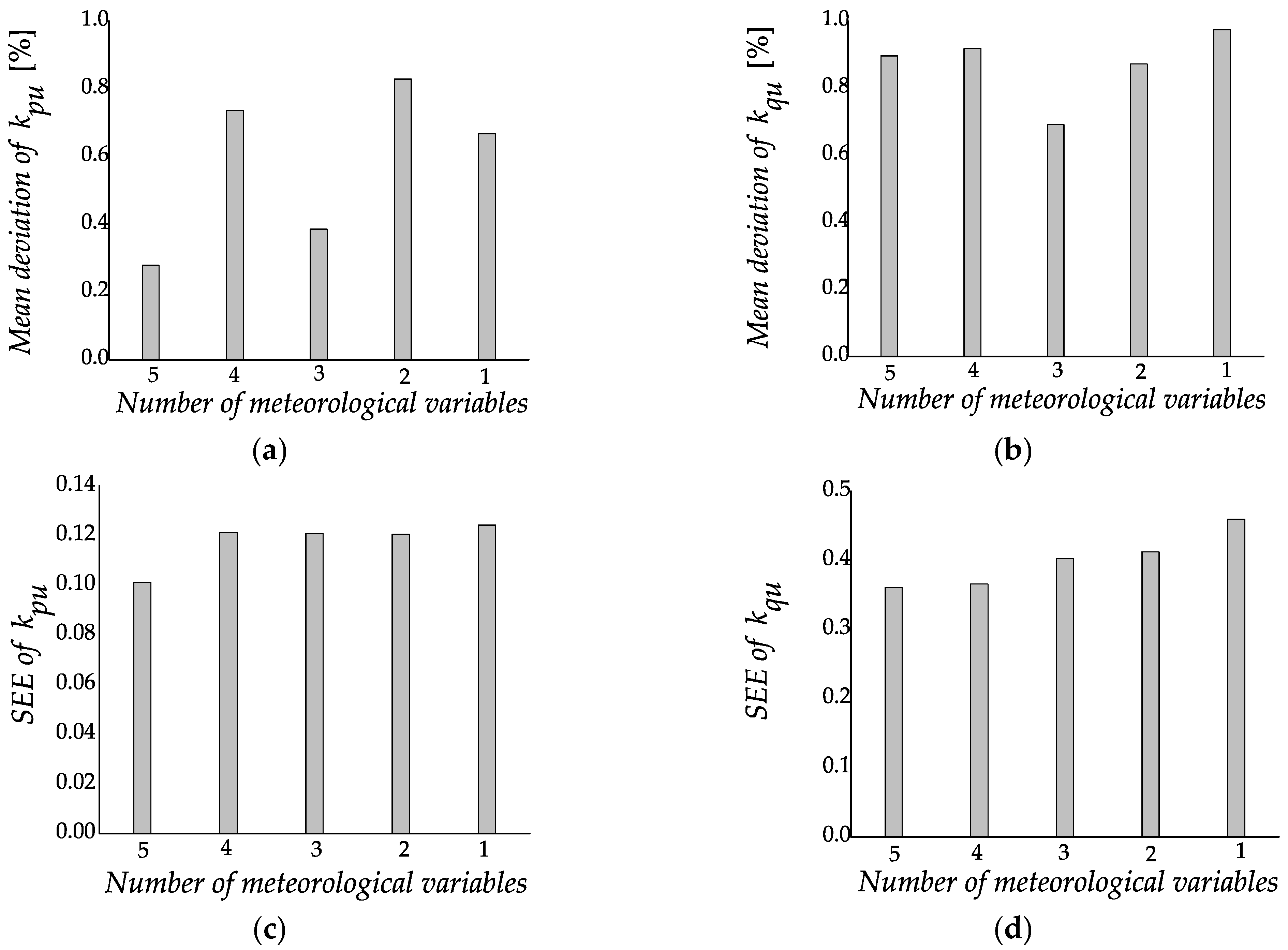
From the 36 comparisons of k_pu values, the following results are obtained. First, in 34 points (i.e., in 94.4% of all comparisons), the deviations of k_{pu_5} values in Table 5 from the corresponding values for fitting curves are less than ±15%. Secondly, in 2 points (5.6% of comparisons), deviations are within the range from ±15% to ±25%, with a maximum deviation of 21.8%. Furthermore, a mean value of all 36 deviations is 0.28%, while the standard error of estimate is 0.101.

A comparison of the parameters k_qu from Table 5 (denoted as k_{qu_5}) with the corresponding k_qu values from fitting curves yields the following number of points within the ranges of deviations: 30 points (83.3% of all comparisons) when deviations are less than ±15%, and 6 points (16.7% of comparisons) when deviations are from ±15% to ±25%. A mean value of all 36 deviations is 0.90%, while the standard error of estimate is 0.361.

3.3.2. Comparison of the Results When Applying Fewer Than Five Meteorological Variables

Generally, when a smaller number of meteorological variables is applied for estimating k_pu and k_qu, somewhat larger deviations from the values in Table 3 are obtained. Thus, when k_pu is estimated from the models with four, three, two and only one meteorological variable, the mean values of deviations are 0.74%, 0.386%, 0.829%, and 0.67%, respectively, while standard errors of estimates are almost the same (around 0.12), and the largest value of 0.124 is obtained when one meteorological variable is used. It means that the best results of k_pu are obtained from the five meteorological variables, and that the simpler models with smaller number of meteorological variables can be used with tolerable errors. For example, the results of the models with only one meteorological variable represented by almost identical k_pu values in particular season (

Table 6. Parameters k_pu and k_qu in different seasons and day intervals calculated from average meteorological variable A_p (k_{pu_1} and k_{qu_1}), of a working weekday, Saturday, and Sunday, as listed successively.

Season	Day Interval	0 h–6 h	6 h–12 h	12 h–18 h	18 h–24 h
Winter	kpu_1	1.47, 1.46, 1.47	1.47, 1.47, 1.46	1.42, 1.46, 1.46	1.47, 1.46, 1.47
	kqu_1	3.87, 3.75, 3.92	3.87, 3.77, 3.69	3.04, 3.17, 2.75	3.31, 3.48, 3.77
Spring/Autumn	kpu_1	1.37, 1.37, 1.36	1.37, 1.37, 1.37	1.36, 1.37, 1.36	1.37, 1.36, 1.37
	kqu_1	3.42, 3.42, 3.41	3.42, 3.42, 3.41	3.40, 3.42, 3.40	3.42, 3.41, 3.41
Summer	kpu_1	1.33, 1.34, 1.33	1.33, 1.33, 1.33	1.33, 1.33, 1.33	1.33, 1.33, 1.33
	kqu_1	3.67, 3.68, 3.68	3.67, 3.67, 3.67	3.66, 3.66, 3.66	3.66, 3.68, 3.66

) and denoted as k_{pu_1}, deviate from the corresponding values from the fitting curves for less than ±15% in 31 points (86.1% of all 36 comparisons), and in 5 points (13.9% of comparisons) deviations are greater than ±15% but less than 23.3%.

Reduction of the number of meteorological variables used for k_qu estimation also has a negative influence on deviations of the estimated k_qu values from the k_qu values that are from fitting curves. Thus, k_qu values obtained by models with four, three, two, and one meteorological variable yield the deviations whose mean values are close to the value obtained when five meteorological variables are used, i.e., 0.92%, 0.698%, 0.87%, and 0.97%, respectively, but standard errors of estimates increase with the reduction of the number of input variables, i.e., 0.366, 0.403, 0.412, and 0.460. Thus, when the simplest models with only one meteorological variable are applied (k_qu values, k_{qu_1}, in Table 6), in 29 points (80.6% of all 36 comparisons) the deviations from the values that belong to k_qu fitting curves are less than ±15%; in 5 points (13.9% of comparisons) the deviations are within the range between ±15% and ±25%, while in another 2 points the deviations are greater than ±25% but less than 32.2%.

Figure 1 summarizes the mean values of deviations (mean deviations) and the standard errors of estimates (SEEs) obtained when different numbers of meteorological variables is used for k_pu and k_qu estimations. The general trends of increased mean deviation of k_pu and standard errors of estimates of both k_pu and k_qu can be seen.

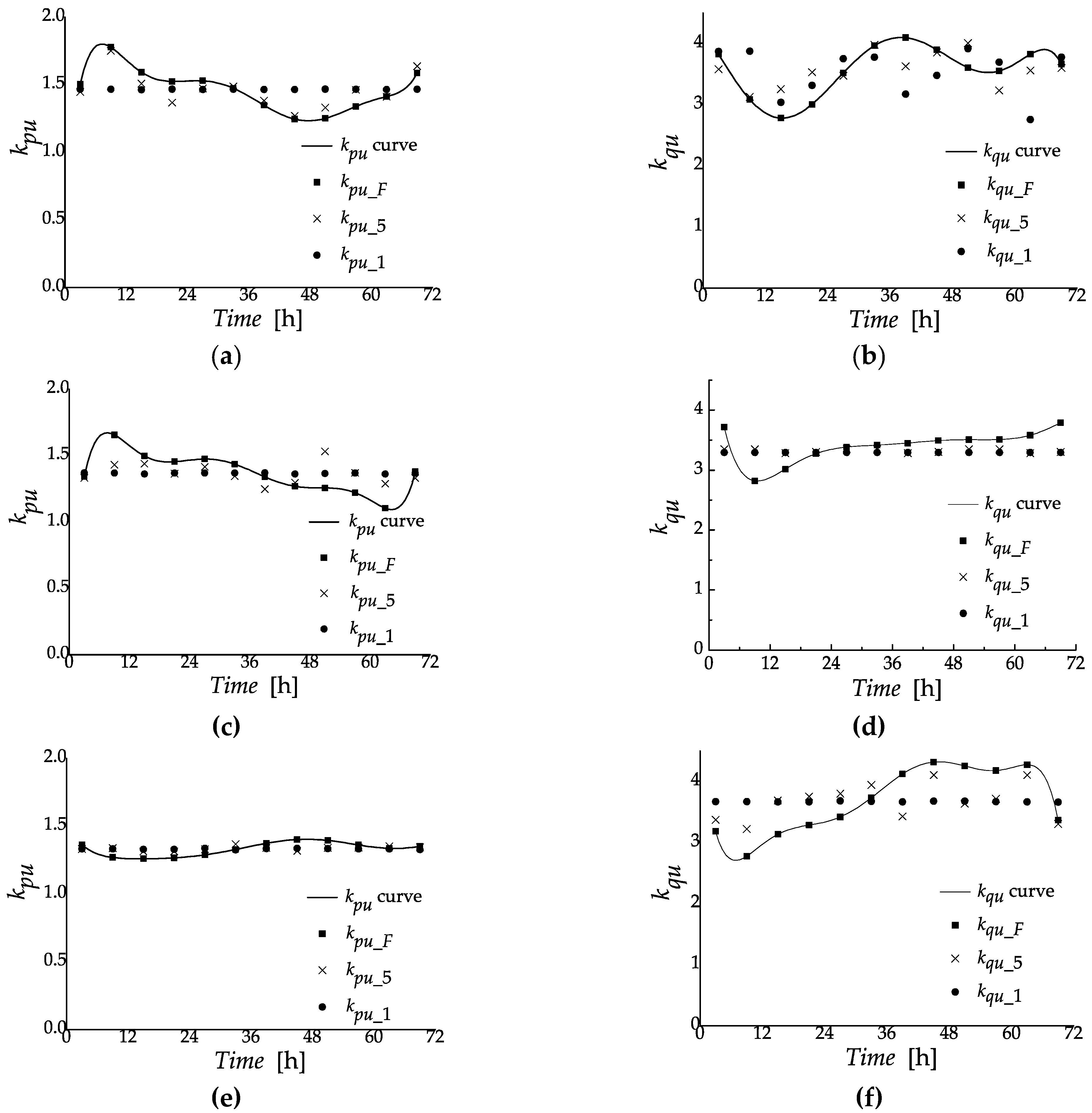
For better insight into the influence of the considered number of meteorological variables on load model parameter estimation, Figure 2 presents the fitting curves of load model parameters, with the corresponding k_pu and k_qu values from these curves, and k_{pu_5} and k_{qu_5}, and k_{pu_1} and k_{qu_1}, for all three seasons. Generally, the values of k_pu are greater in winter and the smallest in summer, no matter what type of variables, i.e., electrical or meteorological, are used for their determination. Taking into account the deviations of estimated values from the corresponding values from the fitting curves (Section 3.3.1 and Section 3.3.2) and Figure 2a,c,e, the meteorological variables can be used for k_pu estimation of the examined demand of administrative buildings. The estimation on the basis of five meteorological variables is more accurate than the estimation by using one meteorological variable.

The applications of different numbers of meteorological variables for k_qu estimation also influence the accuracy of the estimations of k_qu during the year. The most accurate results are also obtained by using five meteorological variables, while the applications of a fewer number of input variables, including the application of only one variable, can be used for only rough k_qu estimations.

3.3.3. Comparison of the Results with the Results Obtained from the Validation Set of Measurements

Further, we checked whether it is possible to use models (7)–(36) for the estimation of load model parameters of the examined demand when electrical variables are not available. For this purpose, the aforementioned validation set of measurements is used, as well as the corresponding average meteorological variables in different seasons and time intervals of any day (values inside parentheses in Table 4). These average values are used to calculate k_pu and k_qu in different seasons from different numbers of meteorological variables, according to (7)–(36), for characteristic days and time intervals.

The values of k_pu and k_qu obtained using one to five meteorological variables were compared successively with averages of corresponding k_pu and k_qu values derived from electrical variables from the validation set of measurements (k_pu and k_qu values inside parentheses in Table 3). In this way, we checked what is the accuracy of the estimates in the case when the electrical variables that are necessary for load model parameter identification are not available. Distributions of the deviations of k_pu and k_qu from the corresponding values inside parentheses were worse than the distributions discussed in Section 3.3.1 and Section 3.3.2. For example, when equations with five meteorological variables are applied, in 30 points the deviations are from 0% to ±15% and in 6 points the deviations are from ±15% to ±25%. When the models with five meteorological variables are used for parameter k_qu determination, in 25, 8, and 3 points the k_qu deviations are in the ranges from 0% to ±15%, from ±15% to ±25%, and from ±25% to ±27.4%, respectively. Similar distributions of deviations for both k_pu and k_qu are obtained when the models with only one meteorological variable are applied.

The mean values of the deviations of k_pu values from Table 3 (inside parentheses) when the models with different numbers of meteorological variables are used are up to 3%, and the standard errors of estimate are in a relatively narrow range from 0.179 to 0.215. These results indicate that the parameter k_pu can be estimated with almost the same accuracy from the presented models with one to five meteorological variables tested in descending order. Rough estimation of k_qu values is also possible, despite the number of used meteorological variables, since the mean value of k_qu deviations from the corresponding values inside the parentheses is less than or equal to 1.83% when different numbers of meteorological variables are used, while standard errors of estimate belong to a relatively narrow range, i.e., from 0.454 to 0.509.

3.4. Estimation by Using Ambient Temperature and Validation of the Results

Since the ambient temperature is the most commonly available meteorological data listed in weather reports, a linear regression is performed in order to obtain relationships between the load model parameters of the examined demand of administrative buildings and the temperature as the only independent variable. Thus, linear regressions for different seasons are applied to datasets of average load model parameter values and the average values of ambient temperatures, in 6 h intervals of a working weekday, Saturday, and Sunday. Thus, the results (37) and (38) are obtained for winter:

$$k_{pu}=1.48384-0.00818T ,$$

(37)

$$k_{qu}=3.58671-0.00755T ,$$

(38)

for spring/autumn:

$$k_{pu}=1.45848-0.00976T ,$$

(39)

$$k_{qu}=3.38635+0.00281T ,$$

(40)

and for summer:

$$k_{pu}=1.34441-5.8545\times {10}^{-4}T ,$$

(41)

$$k_{qu}=3.08539+0.0272T .$$

(42)

Relationships (37), (39), and (41) are obtained with correlation coefficients 0.600, 0.575 and 0.351, respectively, indicating the existence of correlation between ambient temperature and k_pu in all seasons. Linear relationships of k_qu, (38), (40) and (42), are obtained with correlation coefficients 0.500, 0.071 and 0.844, respectively, i.e., there is no correlation between k_qu and ambient temperature only in spring/autumn.

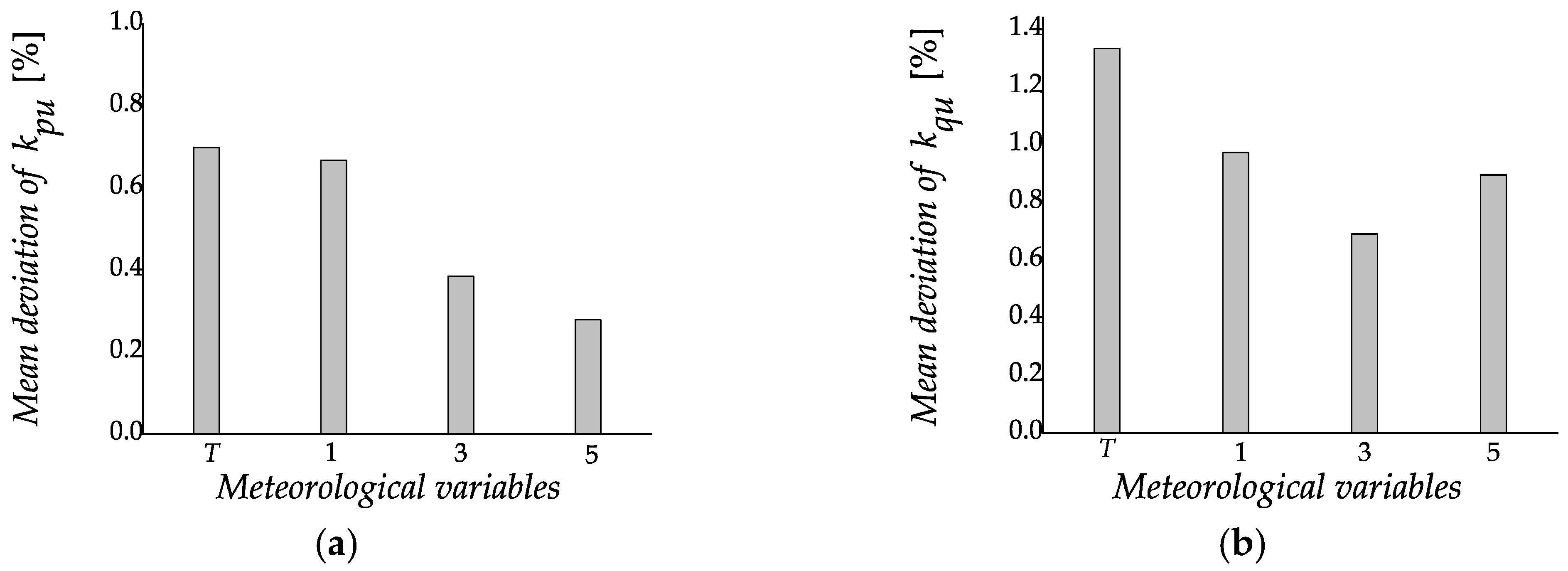
The average values of ambient temperature in particular season, and day intervals of three characteristic days are inserted in corresponding linear relationships, and estimated load model parameter values are obtained. These values are compared with corresponding data from fitting curves, and deviations are calculated. Regarding the distribution of k_pu deviations, in 31 and 5 points the deviations belong to the ranges from 0% to ±15% and from ±15% to ±25%, respectively, while for the distribution of k_qu deviations, in 28, 6, and 2 points the deviations belong to the ranges from 0% to ±15%, from ±15% to ±25%, and from ±25% to ±29.4%, respectively. The mean value of all 36 deviations of k_pu is 0.70%, and standard error of estimate is 0.120, which are similar to values obtained in the cases when less than five meteorological variables are included in linear regression. Mean value of all k_qu deviations is 1.33% and standard error of estimate is 0.426. These values are also similar to those obtained when a smaller number of meteorological variables is applied in k_qu models.

For comparison, Figure 3 presents the mean deviations of k_pu and k_qu when only ambient temperature is applied for parameter estimations, and when the minimum (1), average (3), and maximum number of meteorological variables (5) are used according to the procedure described in Section 2. The mean values of deviations when ambient temperature is used are the largest and the most similar to those when only one meteorological variable is used.

The validation of (37)–(42) is performed in the same manner as explained in Section 3.3.3. The mean value of k_pu deviations is small, i.e., at about 0.49%, and the standard error of estimate is 0.185, which are similar values to the k_pu values from the mentioned section. The mean value of k_qu deviations is 1.77%, and the standard error of estimate is 0.460; these values are also similar to the values obtained during the validation of models with different numbers of meteorological variables. Thus, both k_pu and k_qu can be estimated on the basis of only ambient temperature when the electrical variables that are necessary for load model parameter identification are not available.

4. Conclusions

Unlike other studies that present the results of load model parameter identification from electrical variables, this paper deals with determining the parameters of a static load model from meteorological variables. After assuming linear relationships between load model parameters of an administrative class of customers and meteorological variables, it was found that the voltage exponents of active and reactive power can be estimated from different numbers of meteorological variables during the year. The most accurate estimates were obtained when all five considered meteorological variables were included in the models, resulting in a k_pu mean value of deviations and a standard error of estimate of 0.28% and 0.101, respectively, and a k_qu mean value of deviations and a standard error of estimate of 0.90% and 0.361, respectively.

The results presented in the paper also showed that when lacking time-consuming measurements of the electrical variables in the network, which have to be performed in order to obtain reliable load model parameters, the meteorological variables commonly listed in weather reports can be used for the estimation of static load model parameters. This implies an application of previously established linear relationships between k_pu and k_qu and the meteorological variables for the examined load. The estimation of load model parameters can be also performed by simple linear relationships between load model parameters and ambient temperature. These relationships can be applied instead of more complex linear models with less than five meteorological variables with similar accuracy. In this case, the mean value of deviations of k_pu is 0.70% and the standard error of its estimate is 0.120, while the mean value of deviations of k_qu is 1.33% and the standard error of its estimate is 0.426.

Further research should include an investigation of the influence of meteorological variables on load model parameters of other load classes, as this may provide further guidelines for a fast and simple estimation of load model parameters from nonelectrical variables.

References

- Korunović, L.M.; Sterpu, S.; Djokić, S.; Yamashita, K.; Villanueva, S.M.; Milanović, J.V. Load Parameters Based on Existing Load Models. In Proceedings of the IEEE PES ISGT Europe 2012, Berlin, Germany, 14–17 October 2012; pp. 1–5. [Google Scholar]
- Milanović, J.V.; Yamashita, K.; Villanueva, S.M.; Djokić, S.Ž.; Korunović, L.M. International Industry Practice on Power System Load Modelling. IEEE Trans. Power Syst. 2013, 28, 3038–3046. [Google Scholar] [CrossRef]
- CIGRE WG C4.605. Modelling and Aggregation of Loads in Flexible Power Networks; Rep. TB 566; CIGRE: Paris, France, 2013. [Google Scholar]
- Arif, A.; Wang, Z.; Wang, J.; Mather, B.; Bashualdo, H.; Zhao, D. Load Modeling—A Review. IEEE Trans. Smart Grid 2018, 9, 5986–5999. [Google Scholar] [CrossRef]
- Korunović, L.M.; Rašić, M.; Floranović, N.; Aleksić, V. Load Modelling at Low Voltage using Continuous Measurements. Facta Univ. Ser. Electron. Energ. 2014, 27, 455–465. [Google Scholar] [CrossRef]
- Korunović, L.; Nikolić, B.; Nikolić, D.; Petronijević, M. Load Modelling by using Normal Operation Data. In Proceedings of the ICEST 2011, Niš, Serbia, 29 June–1 July 2011; pp. 473–476. [Google Scholar]
- Retty, H.A. Load Modeling Using Synchrophasor Data for Improved Contingency Analysis. Ph.D. Thesis, State University, Blacksburg, Virginia, 30 November 2015. [Google Scholar]
- Danković, B.; Antić, D.; Jovanović, Z. Process Control–Process Identification; Faculty of Electronic Engineering: Niš, Serbia, 1996. (In Serbian) [Google Scholar]
- Qian, A.; Shrestha, G.B. An ANN-based load model for fast transient stability calculations. Electr. Power Syst. Res. 2006, 76, 217–227. [Google Scholar] [CrossRef]
- Renmu, H.; Jin, M. Composite Load Modeling via Measurement Approach. IEEE Trans. Power Syst. 2006, 21, 663–672. [Google Scholar] [CrossRef]
- Zhao, J.; Wang, Z.; Wang, J. Robust Time-Varying Load Modeling for Conservation Voltage Reduction Assessment. IEEE Trans. Smart Grid 2018, 9, 3304–3312. [Google Scholar] [CrossRef]
- Mota, L.T.M.; Mota, A.A. Load modeling at electric power distribution substations using dynamic load parameters estimation. Int. J. Elec. Power 2004, 26, 805–811. [Google Scholar] [CrossRef]
- Korunović, L.M.; Stojanović, D.P.; Milanović, J.V. Identification of static load characteristics based on measurements in medium voltage distribution network. IET Gener. Transm. Distrib. 2008, 2, 227–234. [Google Scholar] [CrossRef]
- Tang, X.; Hasan, K.N.; Milanović, J.V.; Bailey, K.; Stott, S.J. Estimation and Validation of Characteristic Load Profile Through Smart Grid Trials in a Medium Voltage Distribution Network. IEEE Trans. Power Syst. 2018, 33, 1848–1859. [Google Scholar] [CrossRef]
- Carne, G.D.; Liserre, M.; Vournas, C. On-Line Load Sensitivity Identification in LV Distribution Grids. IEEE Trans. Power Syst. 2017, 32, 1570–1571. [Google Scholar] [CrossRef] [Green Version]
- Marchgraber, J.; Xypolytou, E.; Lupandina, I.; Gawlik, W.; Stifter, M. Measurement-based determination of static load models in a low voltage grid. In Proceedings of the IEEE PES ISGT Europe 2016, Ljubljana, Slovenia, 9–12 October 2016; pp. 1–6. [Google Scholar]
- Korunović, L.M.; Jović, A.S.; Djokic, S.Z. Measurement-based evaluation of static load characteristics of demands in administrative buildings. Int. J. Electr. Power Energy Syst. 2020, 118, 1–8. [Google Scholar] [CrossRef]
- Lam, J.C.; Tang, H.L.; Li, D.H.W. Seasonal variations in residential and commercial sector electricity consumption in Hong Kong. Energy 2008, 33, 513–523. [Google Scholar] [CrossRef]
- Weather2Umbrella History. Available online: https://www.weather2umbrella.com/istorijski-podaci-leskovac-serbia-sr (accessed on 5 May 2020).
- Radmila, N.J.; Mileva, Ž.; Miodrag, L.; Dubravka, P. Basics of Statistical Analysis; Savremena Administracija: Beograd, Serbia, 1989; pp. 276–384. (In Serbian) [Google Scholar]
- Multicollinearity and Other Problems of Linear Regression. Available online: http://www.matf.bg.ac.rs/p/files/69-Multikolinearnost.html (accessed on 3 September 2020).
- Merkle, M. Probability and Statistics for Engineers and Students of Technical Sciences; Akademska Misao: Belgrade, Serbia, 2006. (In Serbian) [Google Scholar]
- OriginLab Tutorials. Available online: https://www.originlab.com/doc/Tutorials (accessed on 8 August 2020).
Figure 1.
Mean values of deviations of (a) kpu, (b) kqu; standard errors of estimate of (c) kpu, (d) kqu. Values are obtained when 5, 4, 3, 2 and 1 meteorological variable is used.
Figure 2.
Fitting curves of kpu and kqu with the corresponding values (kpu_F and kqu_F) in three characteristic days obtained by using electrical variables, and kpu and kqu obtained by using five (kpu_5 and kqu_5) and one (kpu_1 and kqu_1) meteorological variable, in (a,b) winter; (c,d) spring/autumn; (e,f) summer.
Figure 3.
Mean values of deviations of: (a) kpu, (b) kqu; obtained when ambient temperature T and 1, 3 and 5 meteorological variables are used.