
On the Effect of CO2 on Seismic and Ultrasonic Properties: A Novel Shale Experiment


1
Department of Geoscience and Petroleum, Norwegian University of Science and Technology (NTNU), NO-7034 Trondheim, Norway
2
SINTEF Industry, NO-7465 Trondheim, Norway
3
Aker BP, NO-7011 Trondheim, Norway
*
Author to whom correspondence should be addressed.
Energies 2021, 14(16), 5007; https://0-doi-org.brum.beds.ac.uk/10.3390/en14165007
Submission received: 28 June 2021
/
Revised: 10 August 2021
/
Accepted: 12 August 2021
/
Published: 15 August 2021
(This article belongs to the Special Issue Geomechanics Applied to Carbon Capture and Storage)
Abstract
:Carbon capture and storage (CCS) by geological sequestration comprises a permeable formation (reservoir) for CO2 storage topped by an impermeable formation (caprock). Time-lapse (4D) seismic is used to map CO2 movement in the subsurface: CO2 migration into the caprock might change its properties and thus impact its integrity. Simultaneous forced-oscillation and pulse-transmission measurements are combined to quantify Young’s modulus and Poisson’s ratio as well as P- and S-wave velocity changes in the absence and in the presence of CO2 at constant seismic and ultrasonic frequencies. This combination is the laboratory proxy to 4D seismic because rock properties are monitored over time. It also improves the understanding of frequency-dependent (dispersive) properties needed for comparing in-situ and laboratory measurements. To verify our method, Draupne Shale is monitored during three consecutive fluid exposure phases. This shale appears to be resilient to CO2 exposure as its integrity is neither compromised by notable Young’s modulus and Poisson’s ratio nor P- and S-wave velocity changes. No significant changes in Young’s modulus and Poisson’s ratio seismic dispersion are observed. This absence of notable changes in rock properties is attributed to Draupne being a calcite-poor shale resilient to acidic CO2-bearing brine that may be a suitable candidate for CCS.
1. Introduction
Despite its recently gained momentum and level of awareness, how exactly mankind is supposed to overcome the challenge that is the reduction of anthropogenic carbon dioxide (CO2) in the atmosphere is still a question left unanswered. Considered an indispensable technology to reach the Paris Agreement targets among commonly proposed solutions, Carbon Capture and Storage (CCS) has manifested itself as a force to be reckoned with. The International Panel on Climate Change (IPCC) [1] defined CCS as “a process consisting of the separation of CO2 from industrial and energy-related sources, transport to a storage location and long-term isolation from the atmosphere”. The feasibility of geological storage of CO2 is demonstrated [2,3,4] but it is impossible to eliminate all pathways between the subsurface and the atmosphere due to the porous nature of rocks, let alone the wells themselves. Thus, it becomes a question of time as to whether CCS may be considered an option, as the injected CO2 is supposed to remain in the subsurface for the year timescales needed to avoid climate impacts [5,6,7]. In CCS context, geological storages are predominantly reservoir sands enveloped by impermeable shales. This configuration is the primary mechanism for ensuring secure and effective storage.
Mapping the movement of CO2 in the subsurface to demonstrate its secure retention is paramount but it is uncertain whether the integrity of the seal is compromised (and to what extent) due to continued exposure to CO2. Busch et al. [8] identified storage conformance and seal integrity as key in risk of leakage determination as well as storage capacity and injectivity limitations. Kampman et al. [7] named low permeability and capillary entry pressure as two mechanisms that retard CO2 migration. Direct and indirect observations are not only possibilities but also necessities. The former is expensive and technically difficult while the latter (mostly based on seismic surveillance) is both cost-effective and non-intrusive [9]. Seismic monitoring is associated with a certain degree of ambiguity from being influenced by a multitude of factors (e.g., mineralogical composition, porosity, pore fluid, pore pressure, degree of saturation, and in-situ state of stress) [10].
When injected into a reservoir, CO2 displaces the pore fluid (water or brine) and with time either dissolves into the pore fluid or remains as free CO2. It will also react to make more stable phases. Buoyancy generates a plume-like structure due to the concentration of free CO2 at the reservoir-caprock interface, accompanied by a pressure difference that depends on in-situ pressure and temperature conditions [11] for a normal hydrostatic situation. Espinoza and Santamarina [11] provided a threefold explanation of plausible causes of caprock sealing capacity degradation: “(i) hydraulic fracture and fault (re)activation by reservoir overpressure, (ii) aqueous CO2 diffusion into caprock water (without bulk CO2 invasion) and consequent water acidification and mineral dissolution, and (iii) CO2 invasion into caprock, capillary breakthrough, and CO2 advection”. The primary mechanism of cause (i) is alterations in effective stress that may change the mechanical and petrophysical properties of rocks (strength, stiffness, deformation, permeability, and porosity). Cause (ii) is due to concentration gradients combined with pH being inversely proportional to CO2-dissolution, and cause (iii) is prevented when the buoyancy-induced fluid pressure is lower than the capillary entry pressure of the seal.
Other less known coupled processes that could impair the integrity of the seal include [11]: “reactivity of water dissolved in CO2, CO2 intercalation in clays, changes in electrical interaction between clay particles due to water acidification and displacement by CO2, and caprock dehydration and capillary-driven volumetric contraction”. These fluid–rock reactions are ambiguous as mineral precipitation-induced self-sealing phenomena that limit the diffusion of CO2 are numerically predicted, while self-enhancing mineral dissolution and porosity generation that create a continuous increase in transport properties are experimentally observed [7]. CO2-dissolution in brine has been experimentally proven to increase with pressure at given temperature and NaCl-concentration, decrease with temperature for given pressure and brine compositions, and decrease with NaCl concentration for a given temperature and pressure [12,13]. Minerals such as feldspar, calcite, and pyrite may succumb to precipitation and dissolution induced by decreasing pore fluid pH [14]. Chlorite and illite are partly transformed into smectite in the aftermath of interaction with supercritical CO2 (scCO2) [15]. scCO2 also impacts the swelling of shales to a greater extent than pure water and brine [16]. Clay minerals adsorb vast quantities of CO2, with Ca-exchanged smectite adsorbing the most, followed by Na-exchanged smectite, illite, and kaolinite, while the contribution from chlorite is negligible [17]. Since illite and kaolinite also adsorb CO2, adsorption must be a mineral surface phenomenon rather than an interlayer one: most adsorption tests involve powdered specimens in which the surface area in contact with CO2 is significantly increased [18]. Klewiah et al. [19] recently reviewed experimental sorption studies of CO2 (and CH4) in shales where the influence of organic matter, thermal maturity, kerogen type, inorganic components, moisture, and temperature are elaborated.
Uniaxial compressive strength (UCS) experiments on shales exposed to CO2-water or CO2-brine feature a reduction of Young’s modulus E and Poisson’s ratio [16,20,21,22,23,24,25]. If only exposed to scCO2, Choi et al. [25] measured an increased Young’s modulus. Tensile strength is determined by the Brazilian test, in which different shales were found to be both sensitive (decrease and increase in strength) [25,26,27,28,29] and insensitive (constant strength) [30] to CO2 exposure. The common denominator in both experiment types is that the specimens are submitted to mechanical testing at ambient temperature and pressure conditions after being exposed to CO2. Reintroducing specimens to ambient conditions post CO2 exposure could influence their mechanical properties due to microstructure damages caused by CO2 exsolution [31]. It is thus difficult to attribute any observed changes in Young’s modulus and Poisson’s ratio to the effect of CO2 alone. Triaxial compression tests (UCS plus confining and pore pressure) are able to counter these artifacts by maintaining constant temperatures and pressure close to in-situ conditions. Decreasing triaxial strength [26] and increasing Young’s modulus [29] are also measured with increasing scCO2 exposure time. Agofack et al. [32] detected a decrease in Young’s modulus and Poisson’s ratio for a triaxial compressed Draupne Shale. Their results are however inconclusive due to procedural flaws related to limited number of measurements that made statistical analysis difficult, and CO2 exsolution that could affect the undrained bulk modulus via pore fluid compressibility caused by decreasing pore pressure during loading. Choi et al. [25], Al-Ameri et al. [33], Elwegaa et al. [34] measured decreasing ultrasonic P- and S-wave velocities post-CO2 exposure which the two latter converted to decreasing dynamic Young’s modulus assuming isotropy. Lebedev et al. [35] considered anisotropy for their shaley sandstones that also decreased in P-wave velocity upon scCO2 injection into brine-occupied pore space. Consistent with their compressive and tensile strength results, Choi et al. [25] measured increasing P-wave velocity if only exposed to scCO2. Dewhurst et al. [18] reiterated that shale dehydration may alter the rock properties being measured: strength and elastic properties (Young’s modulus and Poisson’s ratio) from triaxial testing are particularly impacted by pore fluid loss. Bhuiyan et al. [31], Fatah et al. [36] neatly summarized CO2–shale interactions in terms of CCS implications.
Upon being recognized as a potential CCS candidate due to its extension over planned CCS reservoirs, Draupne’s mechanical properties are studied in the absence and presence of CO2 [32,37,38,39]. Draupne Shale is associated with high capillary sealing (from a permeability viewpoint) but Skurtveit et al. [37] questioned its formation and sealing capacity by indirect tensile strength and undrained shear strength experiments. Zadeh et al. [38] observed increasing P- and S-wave velocities but decreasing Thomsen’s parameters with increasing mean effective stress. To the best of our knowledge, Draupne’s mechanical properties are unprobed at seismic frequencies. It is also unexplored at different fluid exposure phases (including CO2 exposure) over an elongated period of time within the same experiment.
Most studies involve post-CO2-interaction experiments at ambient conditions devoid of CO2 in its experimental condition at either subseismic or ultrasonic frequencies. There is a paucity of studies involving CO2 experiments under continuous in situ conditions at seismic frequencies. We present a method to monitor the mechanical responses of a specimen exposed to CO2 over an elongated period of time using the forced-oscillation (FO) and pulse-transmission (PT) techniques. PT is the dominant dynamic technique but FO and resonant bar (RB) studies also exist albeit limited to sandstones exposed to CO2 [40,41,42,43,44,45]. The novelty of our approach is that our specimen is exposed to three different fluids while confined under continuous stress, pressure, and temperature regimes. We attempt to answer the question whether CO2 changes the mechanical properties of a caprock and thus present a risk for efficient, long-term containment in the reservoir below. To this end, we determine whether Draupne Shale is suitable candidate for CCS by monitoring Young’s modulus and Poisson’s ratio at seismic as well as P- and S-wave velocities at ultrasonic frequencies over 575 h. Since no significant changes are observed, Draupne Shale may be a suitable candidate.
2. Theory
2.1. Anisotropy
Anisotropic or isotropic is the material whose elastic properties change or do not change with direction. Anisotropy in shales is caused by the alignment of minerals (particularly clays). The number of independent stiffnesses for anisotropic rocks exceeds the two required to describe isotropic rocks: shales are commonly considered to be transversely isotropic (TI) which increases this number to five [10]. Hooke an theory relates stress and strain (notation for TI symmetry by Voigt [46]) via “ut tensio, sic vis” [47] as
with , , , , and being the five independent stiffnesses. Triaxial cells generate biaxial stress conditions () with confining pressure and axial stress , which enable the determination of all five stiffnesses if three differently oriented samples are considered. To this end, 0 and 90° specimens are required, whereas the third specimen orientation is not required to be 45° but often is for consistency. Thomsen [48] defined three anisotropic parameters to simplify anisotropy
where and denote P- and S-wave anisotropy, while is referred to as the moveout parameter (a critical factor that depends on the shape of the wavefronts). implies isotropy for these dimensionless, ratio-based parameters.
2.2. Cole–Cole Model
Ref. [49] extended the Cole–Cole model [50] from the realm of dielectric constants of liquids to the realm of viscoelastic rocks with a distribution of relaxation times
with and being the real and imaginary parts of the complex modulus ; and its low- and high-frequency (or relaxed and unrelaxed) limits. Not to be confused with any specific modulus, M is a general modulus. with being the angular frequency and being the characteristic time. describes the width of the distribution of relaxation times. reduces it to the underlying Debye model [51]. M is the magnitude of the modulus and is its corresponding attenuation
If the application of the Cole–Cole model for anisotropic rocks is a valid assumption (the anelasticity satisfies the Kramers-Kronig relations (KKR) [52,53], the system is linear, and the attenuation can be described by a single mechanism), it is possible to use this model to perform a qualitative fit based on mathematically solving a least-squares function [49,54,55].
3. Materials and Methods
The versatile nature of our apparatus accommodates simultaneous FO and PT measurements at seismic and ultrasonic frequencies, respectively. Strain amplitudes between and apply not only to FO and the field but also to PT [56,57].
3.1. Mechanical Measurements
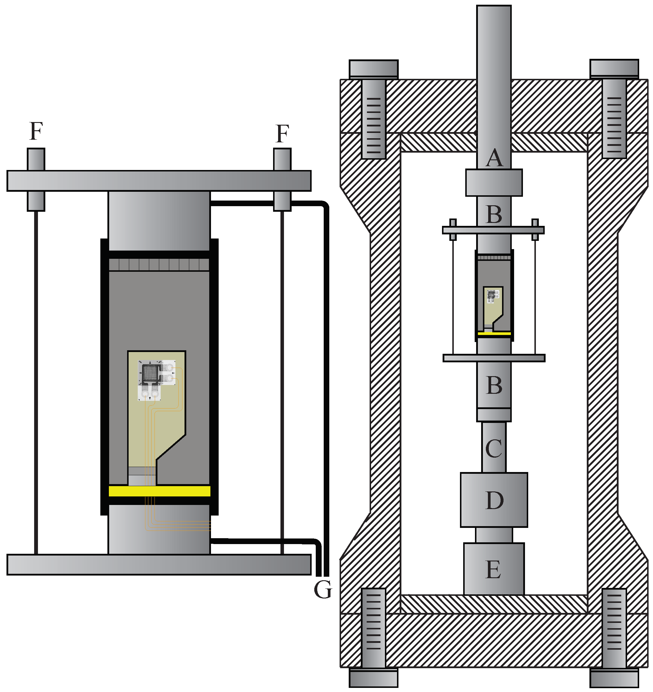
Szewczyk et al. [58] described the apparatus as “a technique for the complete characterization of the frequency-dependent elastic properties of anisotropic rocks under stress”. It was designed to accommodate specimens with 2.54 cm diameter and 5.08 cm length. To this end, (i) quasistatic specimens deformations, (ii) Young’s modulus and Poisson’s ratio [49,54] at seismic frequencies, and (iii) P- and S-wave velocities [59,60,61,62] at ultrasonic frequencies are measurable at different temperature, stress, and pressure conditions (Figure 1). Stress and pressure are controlled by an electromechanical frame (MTS Criterion C45 300 kN) and high-accuracy pumps (Vindum VP-Series), respectively. A CO2 flow loop (described in Section 3.4) enabled CO2 effects to be studied [44,45].
3.1.1. Forced-Oscillation (FO) Measurements
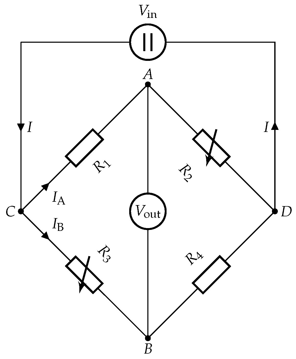
Five Stanford Research SR850 lock-in amplifiers (internal sampling rate of 256 kHz) measure amplitudes and phases of harmonic signals. Uniaxial-stress modulations are generated by a piezoelectric actuator (PI P-235.1S) controlled by a sinusoidal reference signal from one lock-in amplifier and amplified by a voltage amplifier (PI E-421). A piezoelectric force sensor (Kistler 9323AA combined with Kistler 5015A) measures the resulting force signal returned to the lock-in amplifier which determines its amplitude and phase shift relative to the reference signal. Four biaxial strain gauges (Micro-Measurements CEA-06-125WT-350) with eight different gauge elements (four axial and four radial) are connected to four unbalanced Wheatstone bridges [64]. Each Wheatstone bridge is connected to two equidistantly strain gauges elements 180° apart (Figure 2) which averages the signals from both. Four lock-in amplifiers (two axial and two radial) measure amplitudes and phase shifts of the resulting strain signals relative to the reference signal. Axial stress plus axial and radial strains ( is or ) are then
where F, A, , , and are force (amplitude multiplied with sensitivity ), cross-sectional area, measured voltage signals across the unbalanced Wheatstone bridges ( is total axial or radial amplitude), input activation voltage, and gauge factor, respectively. Note that circumferential strain is equal to radial strain () within the isotropic plane of an TI medium: and are used for simplicity. Averaging multiple strain measurements at different positions approximates the bulk mechanical properties of a rock [65]. All recordings from the lock-in amplifier are simultaneously sampled by an in-house acquisition software designed to detect stability (within a pre-defined tolerance) and average up to 50 recordings.
Young’s modulus [66] and Poisson’s ratio [67] as electrical signals transformed into mechanical responses become
in which and since only a 0° specimen is considered (Figure 3). Equation (12) combines Equations (10) and (11) to provide the total amplitude from the stress–strain hysteresis loop (e.g., Lakes [68]). However, since phase shifts for shales are small [69,70,71,72], . Since the force sensor and strain gauges differ in electronic circuitry, electronics-induced phase shifts are greater than the rock specimen-induced ones [58]. Attempts to use an aluminum standard as force sensor [54] with similar circuitry were temporarily abandoned [73,74] until a design flaw causing unreliable phase measurements due to minor misalignments [75] was ultimately discovered [76].
3.1.2. Pulse-Transmission (PT) Measurements
Four P- and S-wave piezoceramics (500 kHz) integrated in both endcaps measure P- and S-wave velocities based on the time of flight principle
where L is the specimen length, t is the travel time, and is the system travel time. The ultrasonic signals are acquired by a system comprising a signal generator (Agilent 33220A), an amplifier (T&C Power Conversion AG 1017L), a switch unit (Agilent 34970A), and an oscilloscope (Tektronix TDS3012B) that are connected to a computer and controlled by another in-house software that also stores the data. The sampling frequency is 10 MHz. To improve the signal-to-noise ratio, the amplified ( dB) waveforms are averaged (64 times) by the oscilloscope. is either or which combined with density yields
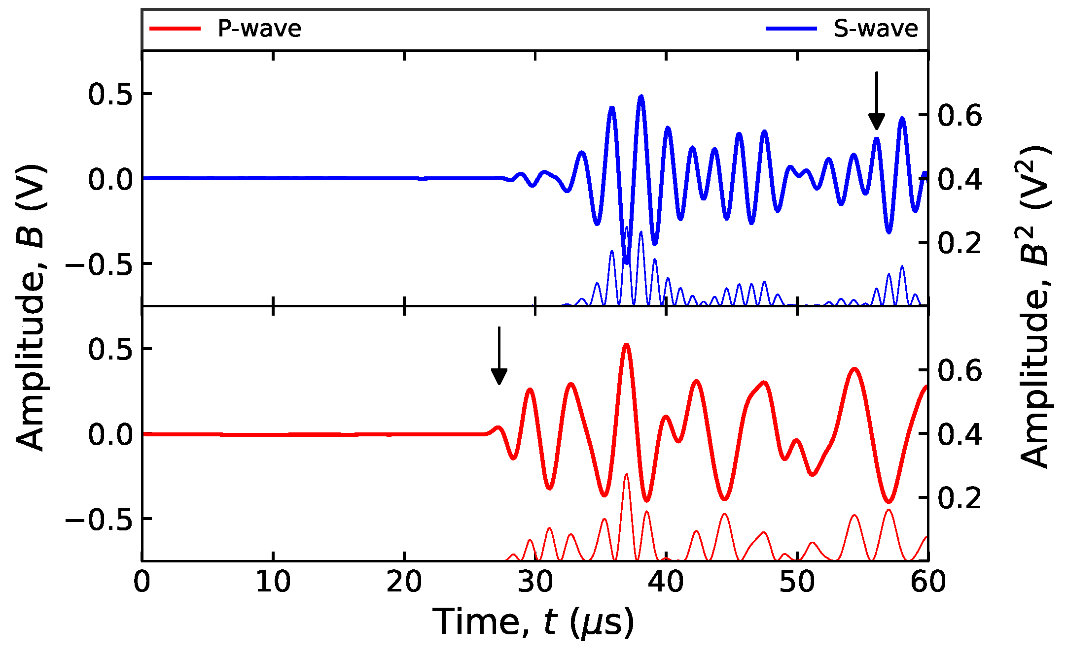
with 0 implying the considered 0° specimen (Figure 3) and its corresponding stiffnesses and . Figure 4 exemplifies P- and S-waveforms at 500 kHz. Szewczyk et al. [77] described the arrival picking procedure in which aluminum 7075 was used for calibration purposes. The S-wave signal is disfigured by faster P-waves that spawn from initial S-waves at every acoustic impedance interface. There is thus more ambiguity in picking the first S- than P-wave arrivals.
3.2. Draupne Shale
In the ongoing large-scale CCS demonstration project in Norway, several potential storage reservoirs have been chosen in the vicinity of the Troll gas field. Draupne Shale is the caprock in this area [78]. The specimen used herein originates from well -3S within the Ling Depression located in the central North Sea [32,37,38,39]. Considered an anisotropic and homogeneous shale, Zadeh et al. [38] described the Draupne Formation while investigating specimens from the same well as this study. Table 1 and Table 2 tabulate Draupne’s pre-CO2 exposure mineralogical composition and physical properties. Extracted from a 13.0 cm interval between 2574.86 and 2576.99 m depth, the specimen experienced minimum exposure to ambient conditions due to our accelerated mounting procedure. Diffusion time was reduced by drilling a 1.50 mm hole along its axis at the center of the specimen that also reduced the diffusion length from 12.7 to ∼6 mm. Since we measure local strains at the surfaces of the specimen, we assume that this action has negligible effect on the overall stiffness of the material.
3.3. Experimental Protocol
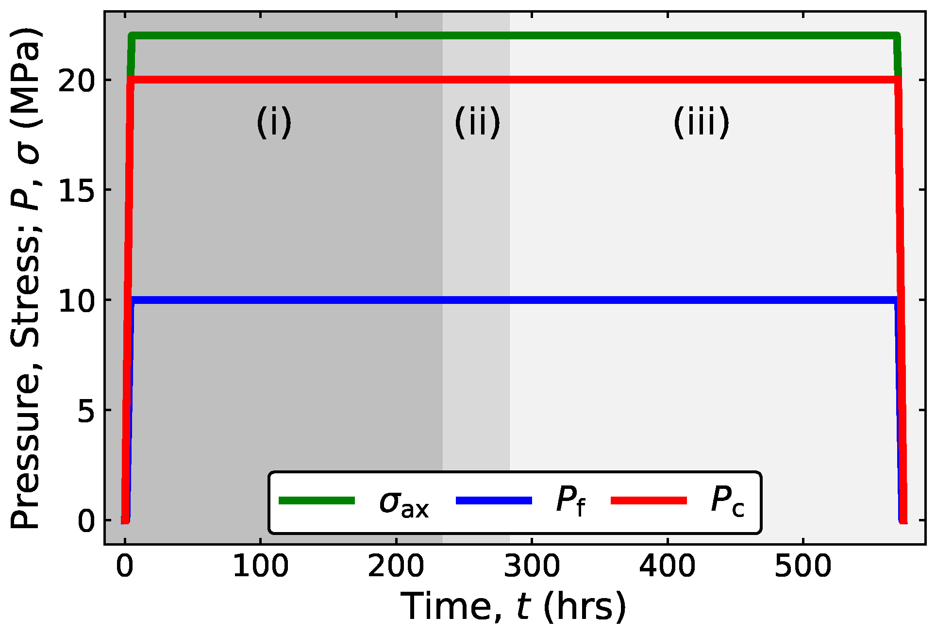
Although our apparatus is able to perform measurements at elevated temperatures [79], the current experiment occurred at room temperature to concentrate on CO2-driven mechanisms that may influence the mechanical properties of our specimen. Confining pressure , pore pressure , and axial stress were kept constant, respectively, at 20, 10, and 12 MPa from the outset and throughout (Figure 5). Adequate system–specimen coupling is ensured by a finite deviatoric stress ( MPa). The specimen was left to consolidate while LVDTs and strain gauges were constantly monitored and analyzed before initiating FO. Three fluid exposure phases are implemented: constant pressure without (closed system for the specimen to consolidate (Phase (i))) and with fluid flow (open system regulated by a back pressure connected to a pump administrating brine (Phase (ii)) or the CO2 flow loop (Phase (iii))) at mL/min. Fluids are distributed around the specimen by a surrounding mesh, two sintered plates at each specimen–endcap interface, and the hole at its center. In other words, there is no flow through the specimen but instead around it and within the hole. For all intents and purposes, roman numbering indicates the respective phases of flow in terms of the previously defined (i), (ii), and (iii) in all graphs with time as the x-axis (exemplified by Figure 5). Three dynamic test procedures were planned and executed with the objectives being to (a) monitor the elastic response of our specimen at a constant frequency with time, (b) complete dispersion characterization tests with frequency before and after the former, and (c) PT recordings at ultrasonic frequencies:
- (a)
- Frequency sweeps were performed once the specimen was adequately consolidated (by analyzing deformation) in order to identify the optimal frequency to be used for the duration of the experiment. 25 Hz was proven to generate the optimum signal with a sampling interval of 60 s to constrain the data size.
- (b)
- A total of three dispersion tests (full frequency sweeps from 1 to 144 Hz) at two different exposure phases were sequentially conducted: (i) and (ii) during consolidation in Phase (i), and (iii) at the of end of the experiment in Phase (iii).
- (c)
- A third test was also simultaneously executed as P- and S-wave ultrasonic signals were recorded every 900 s during the entirety of the test.
3.4. CO2 Flow Loop
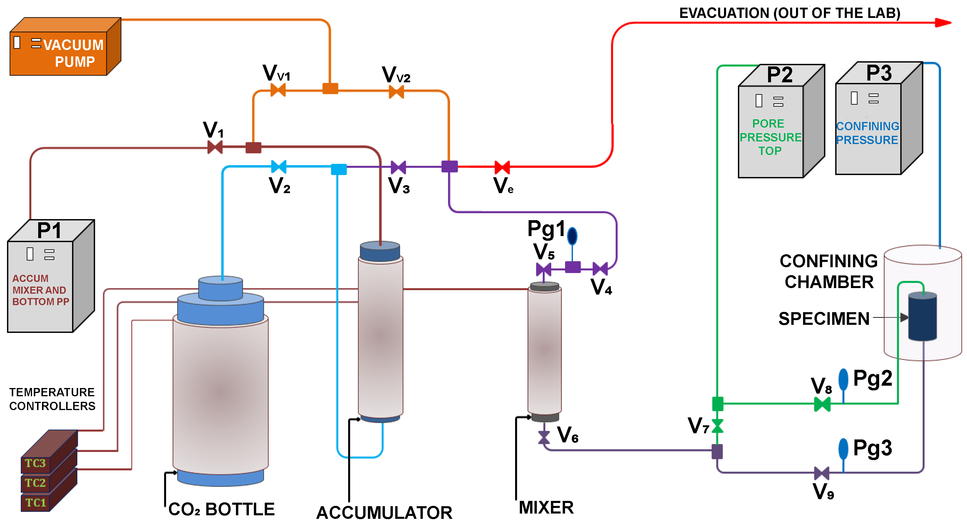
The CO2 flow loop system comprises a CO2 container ( L capacity), an accumulator (1 L capacity), a mixing unit (1 L capacity), two pumps (Quizix and vacuum), as well as three Eurotherm temperature controllers (Figure 6) [44,45]. Integrated in the accumulator is a movable seal membrane that separates CO2 in the lower part from oil in the upper part. The mixing unit was filled with 80% brine of wt% NaCl concentration. CO2 exsolution during wave-induced pressure changes is prevented by heating the mixing unit to 40 °C for the brine to be slightly undersaturated with CO2. All parts of the mixing unit and flow loop are evacuated using the vacuum pump pre-CO2 introduction. Closing valves Vv1, Vv2, V6, and Ve plus opening valve V2 allow for both the accumulator and mixing unit to be filled with CO2 to a pressure corresponding to that of the CO2 container (10 MPa). When valve V2 is closed, CO2 is forced by pump P1 into the mixing unit due to the increased top pressure in the accumulator. CO2 diffusion is facilitated via manual rotation (±90°) of the mixing unit during the mixing process in which CO2 is administered by pump P1 at a pressure equivalent to the pore pressure . CO2 dissolution into brine coincides with a pressure drop observed on pressure gauge Pg1. To counter this pressure drop, valve is reopened for the mixing unit to be re-pressurized by injecting additional CO2, whereupon it was re-rotated back and forth 50 times. This procedure was repeated until the pressure drop was less than 1%. Once the brine was fully saturated with CO2 at elevated temperature, the mixing unit, accumulator and pump P1 were connected and kept at constant pressure equal to and temperatures greater than the FO apparatus.
3.5. Error Analysis
Rørheim et al. [79] elaborated on the potential errors associated with FO. Systematic errors in strain and stress measurements are caused by misalignments, heterogeneities, bulging, deviations from TI symmetry, electronic noise, temperature and transverse sensitivities, cross-sectional changes, Wheatstone bridge input voltage, and strain gauge curvature and possible slip. Random errors in Young’s modulus and Poisson’s ratio correlate with that of the axial and the radial strain amplitudes and . FO measured Young’s moduli and Poisson’s ratios errors are and , respectively. PT depends on three variables—L, t, and —defined by Equation (14). Ultrasonic errors are primarily related to t but also secondary to and tertiary to L. t and are based on the accuracy of the manual waveform picking in which t is more erroneous than . L depends on the precision of the LVDTs. Possible transducer-bedding misalignments are also potential sources of error. PT measured ultrasonic velocity relative errors are estimated to be between and .
4. Results
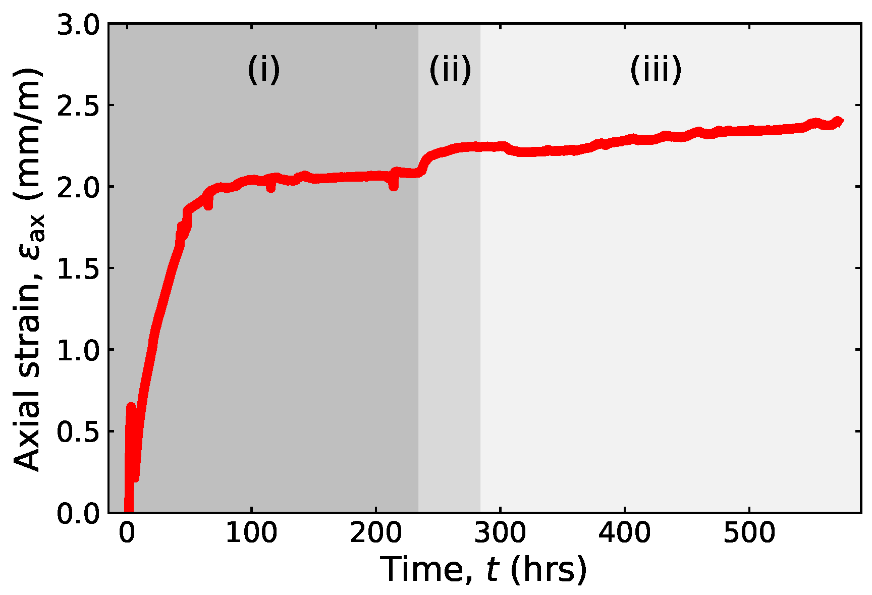
Draupne’s mechanical properties are determined by three independent measurements integrated into a single test with another three different phases of fluid exposure applied under identical stress, pressure, and temperature conditions. The duration of Phases (i), (ii), and (iii) as well as their impact on the axial strain are featured in Figure 7. Phase (i) is categorized into two dominant features based on the expansion rate of the specimen: rapid expansion from 4 to 70 h after the desired pressure and stress levels are enforced, and slow expansion after 70 h until the initiation of the next phase. Phase (ii) is similar to Phase (i) in trend but not in amplitude since the specimen also initially expands before it eventually slows down again (at a lower rate than the previous phase). Phase (iii) saw an initial decrease in as CO2 was introduced at 283 h. Compaction turned into expansion at 320 h, whereupon the specimen expanded at a continuously decreasing rate until the end of the experiment.
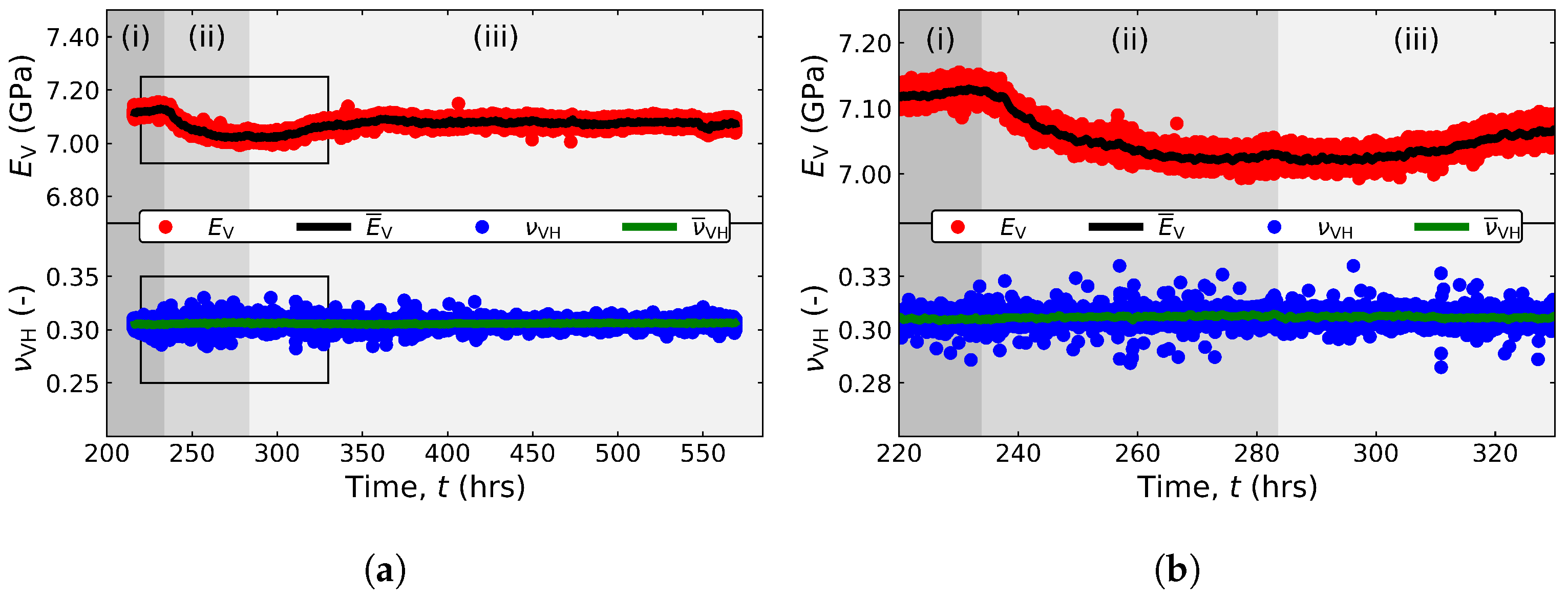
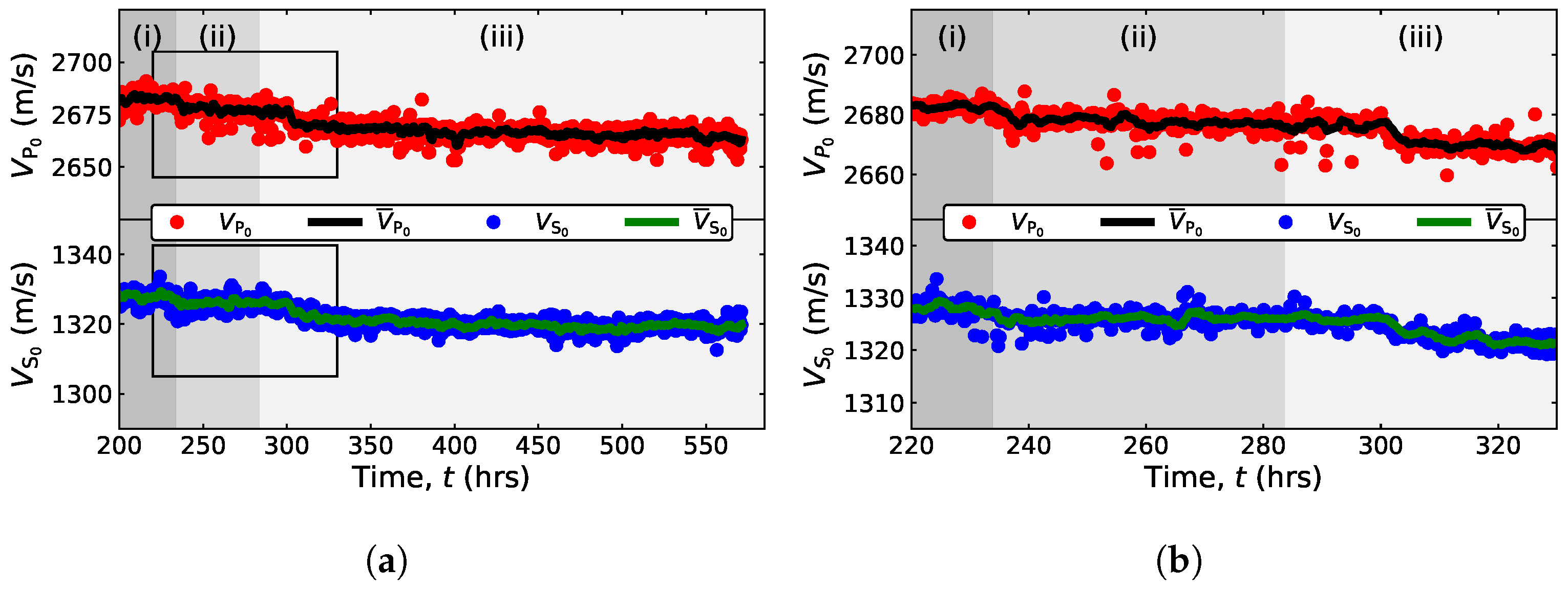
Figure 8 features Young’s modulus and Poisson’s ratio as a function of time: (a) includes the entire experiment while (b) is superimposed from 220 to 330 h with narrower y-axes. As the signals are stabilized with time (Figure 8b), subsequent phases are sequentially initiated. Phase (i) is primarily used for stability and as reference to determine changes in mechanical properties. Phase (ii) introduced at approximately 234 h decreased by %. Phase (iii) introduced at 283 h had an initial stiffening effect ( increased by %) for the first 80 h after influx before plateauing at 364 h with approximately constant until the end. Poisson’s ratio remained resilient to the different phases as a function of time without any noteworthy changes. Figure 9 includes ultrasonic P- and S-wave velocities at 500 kHz recorded every 900 s for the entirety of the test. Despite an accelerated reduction after introducing the brine–CO2 combination, a proclivity towards steady declination of both and is the noteworthiest feature during all three phases.
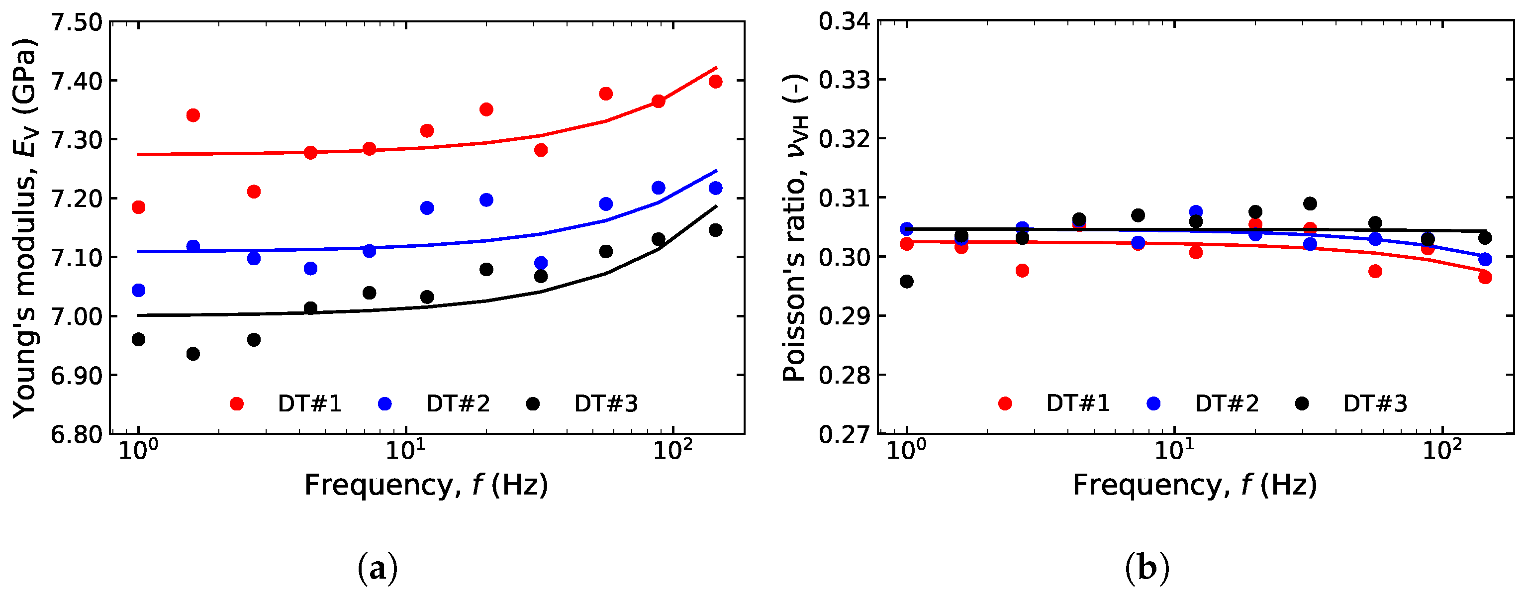
Dispersion is a phenomenon that is a common feature in fluid-saturated rocks. DT#1, DT#2, and DT#3 (dispersion tests numbering from 1 to 3) were executed at 43, 64, and 570 h, respectively. In other words, DT#1 and DT#2 occurred at the initial stage of Phase (i) plus DT#3 at the tail-end of Phase (iii). No dispersion measurements were conducted during Phase (ii) in order to continuously focus on changes in and at 25 Hz. Despite being reduced in terms of magnitude (DT#1 eclipses both DT#2 and DT#3) as a function of time, regression reveals that seismic dispersion appears unaffected by CO2 exposure, with the increase from 1 to 144 Hz being within –. Figure 10b shows Poisson’s ratio as a function of frequency without any noteworthy aspects in need of elaboration beyond the evident continuity.
5. Discussion
5.1. Analysis
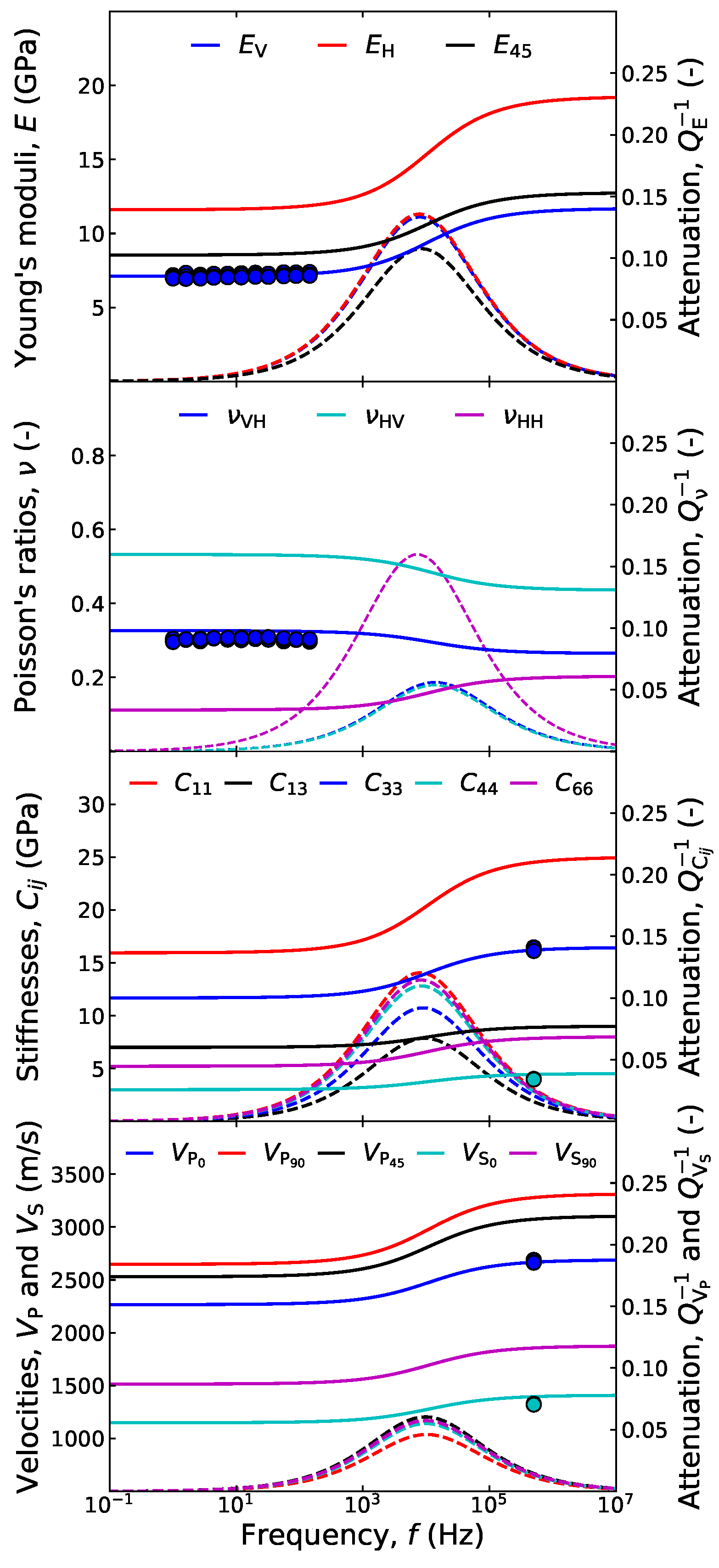
Cole–Cole modelling is a mathematical solution to a physical problem that estimates dispersive properties at unprobed frequencies. Figure 11 combines these assumptions with a least-squares-based joint-fit routine [79,80] which uses , , , , and at and plus Cole–Cole’s and as fit parameters. Fit ambiguity is related to the limited input data: the more inputs, the less ambiguity. Since there are no common parameters measured at both seismic and ultrasonic frequencies, the model is constrained by assuming and to be true [81]. Figure 11 features (until now undefined) anisotropic Young’s moduli , , and , Poisson’s ratios , , and , and P- and S-wave velocities ( is P or S depending on ± being + or − and is 0, 45, or 90)
where , , , , and are the predefined stiffnesses. Figure 11 also includes (absolute value) Cole–Cole modeled attenuation (dashed lined) to compliment dispersion (solid lines) but remains unelaborated due unreliable phase measurements (caused by minor misalignments [75]) that were later resolved [76,80].
5.2. Interpretation
Achieving full saturation is challenging for any field specimens submitted to laboratory experiments. Shale specimens expand when exposed to brine irrespective of the activity of the exposed fluid and pore fluid [82]. Figure 7 shows initial expansion (at ambient conditions) explained by the adsorption of water. Despite briefly being mechanically compacted, the specimen begins to swell again probably due to continued adsorption of water. The specimen eventually becomes fully saturated and the swelling rate subsides at approximately 100 h. Aside from water adsorption, since the osmotic membrane efficiency of shales is typically low, it is possible that ions are simultaneously allowed in and out. However, the effect of ion movement on shale swelling is lower than water adsorption [82]. It is difficult to replicate formation brines synthetically [29]: pore fluid disequilibrium may cause swelling- or shrinkage-induced damage to shales [83,84]. Osmotic pressure-induced changes caused by significant differences in ionic concentrations close to the clay surfaces and in the pore fluid [85] may thus be triggered. Smectite is predominantly prone to osmotic processes. The difference between synthetic and native pore fluid is, however, assumed to be insignificant with osmotic swelling only playing a minor part in the observed swelling. Moreover, Ewy and Stankovic [86] found that sufficient effective stress prevents chemically induced swelling which is an indication that water adsorption in an undersaturated shale is the main mechanism.
Santos and da Fontoura [87] argued that the observed swelling of laboratory shale specimens comprising all types of clay minerals is caused by surface hydration relatable to the amount and distribution of water within the shale. Overall electrical neutrality in fluid–clay interaction is maintained by the distribution of the cationic fluid being concentrated at the surface of the anionic clay particle. Universal for all types of clay minerals is the resulting layer named the diffuse double layer (DDL) that may induce swelling because the adsorbed layer thickness surrounding the clay particles increases [88]. Schaef et al. [89] observed shrinkage of the interlayer spacing at higher hydration states corresponding to shallow burial depths. Compaction turned into expansion at 320 h, whereupon the specimen expanded at a continuously decreasing rate until the end of the experiment. Clay minerals charged with CO2 experience different levels of swelling depending on their water content and interlayer cations [8]. CO2 adsorption within the smectite interlayer is believed to be the main contributor causing the observed swelling. CO2 adsorption capacity may affected by decompaction during coring. Best fit to in situ adsorption conditions is however ensured because the specimen is at in situ stress conditions before being exposed to CO2.
Based on previous studies, Young’s modulus and Poisson’s ratio [16,20,21,22,23,24,25,32,33,34], tensile strength [25,26,27,28], and P- and S-wave velocities [25,33,34] generally decrease with CO2 exposure. Reductions with CO2 exposure are primarily attributed to adsorption-induced swelling of clay minerals and dissolution-induced pore structure changes primarily affecting calcite but secondarily also feldspar. A common denominator is that these shales are calcite-rich. Exceptions that prove the rule do however exist: constant or increasing Young’s modulus and Poisson’s ratios [25,29], tensile strength [25,29,30], and P- and S-wave velocities [25]. Dewhurst et al. [29] considered stiffening and strengthening caused by dissolution and re-precipitation of minerals unlikely and instead opted for an explanation involving water loss. It appears as though it depends on whether (i) or not (ii) CO2 coexists with water or brine: (i) softening and weakening are explained by dissolution being more dominant than precipitation but (ii) stiffening and strengthening are instead attributed to water dehydration. CO2 and water or brine coexistence implies lower pH. Choi et al. [25] measured both increments and decrements depending on (i) or (ii) being enforced.
and changes at 25 Hz are observed to be minimal irrespective of phase: is slightly affected and is virtually nonaffected (Figure 8). In fact, the overall reduction of amounts to less than and occurs during Phase (ii) before CO2 is introduced during Phase (iii). Figure 9 is comparatively different due to and constantly decreasing during all phases. is related to and in the sense that greater stiffness typically implies higher velocities. Temperature outside the sleeve has been recorded in previous tests but was not a priority in this test due to it being found to only vary by ±0.25 °C. and from hypersensitive strain gauges are more likely to be affected by temperature than and from piezoceramics if the temperature-elevated mixing unit imposes temperature variations at specimen level. It is, however, unlikely that temperature variations of these small magnitudes would amount to great errors. DT#1 and DT#2 are thought to provide stiffer responses than DT#3 due to the rapid expansion of our specimen observed until 70 h in Figure 7. Neither stiffening nor weakening appears to affect the seismic dispersion (Figure 10) though. It is, however, unknown whether the dispersion at unprobed frequencies (between seismic and ultrasonic) is affected or also remains unaffected. Dispersion is notably sensitive to fluid mobility: small permeability or viscosity changes could explain seismic and ultrasonic and behaving differently. Since it is unobserved at seismic frequencies, the Cole–Cole model (Figure 11) is unaffected. Bound water with finite shear stiffness [90,91] and enhanced viscosity [90,92,93,94] could also possibly be affected by CO2. Other possibilities are differing pH values for the different fluids, amount of diffusion into the shale bulk, associated changes in surface energy, and desiccation effects.
Neither and nor and are greatly impacted by the different fluids for reasons that remain unclear. CO2 was expected to change the properties [95] to a greater extent than what is observed but was perhaps limited due to Draupne’s lack of calcite and feldspar (Table 1). and plus and are also close to the experimental errors which questions as to whether the changes are physical or artificial. It is, however, an indication that Draupne Shale is suitable for CCS purposes because the changes would not be as negligible if its integrity was greatly impacted. If neither dissolution nor precipitation is dominant but instead they counteract each other, no significant stiffness or strength changes would be observed. Changes in stiffness need not be of the same sign as changes in compressive strength: loss of point cementation at grain contacts with no loss of large volumes of minerals or grains may lead to a weaker bulk but stiffer specimen if finer material is trapped in the pore volume. Time is another aspect to consider because our 24-day experiment is incomparable to in situ timescales. Despite the length scales also being incomparable, diffusion is a notoriously slow process at any scale. Figure 11 is one out of an infinite number of solutions. and are criteria that most shales obey although exceptions do exist [96]. The amount of data obtainable from a single specimen is, however, shown. It is by no means any substitution from performing all three experiments (0, 45, and 90 specimens) required for full characterization assuming TI symmetry but it still offers valuable information. In situ caprock shales are also mostly 0 relative to the reservoir rocks they cover.
Interesting is also the duration of this experiment despite being incomparable to in situ timescales. To our knowledge, it is the longest FO experiment with its 575 operational hours. It was also the only known experiment that performed FO measurement as a function of time instead of frequency at its time of completion. Our primary intention is to describe a technique that monitors changes in elastic properties at seismic and ultrasonic frequencies with time. As such, it is analogous to time-lapse (4D) surveillance in the field. Continuous FO and PT measurement over time could also be extended to conventional creep measurements in the absence of CO2. Chavez et al. [97] later studied FO-measured creep effects on a limestone, a sandstone, and a shale at 2 Hz but at room-dry and uniaxial conditions. Instead of 575 h, they measured for 120 h. It appears as though they did not consider anisotropy because they did not specify the orientation of their Eagle Ford Shale and only included isotropic calculations. They did, however, specify that the largest observed changes occurred in their shale. These results were later also included in Mikhaltsevitch et al. [71].
6. Conclusions
We propose using FO and PT for simultaneous and as well as and measurements over an elongated period of time (in the presence and in the absence of CO2) at constant seismic and ultrasonic frequencies. Three successive phases of fluid exposure are implemented without exposing the specimen to ambient conditions between phases during a single 575 h experiment. This method provides a better understanding of in situ versus laboratory measurements because both frequencies are simultaneously probed at in situ pressure conditions despite the omnipresent up-scaling issue. Shale-dehydration that may alter the rock properties as a consequence of exposure to ambient conditions is avoided because pore fluid loss is eliminated (except during the initial mounting). Draupne Shale appears to be resilient to CO2 exposure as its integrity is neither compromised by notable and nor and changes. CO2 appear to not impact the observed and dispersion beyond minor amplitude variations with time. These changes are attributed to the initial swelling of the specimen. CO2 dissolved in brine is acidic and thus prone to primarily dissolve calcite. However, calcite is a diminutive component of Draupne Shale which could explain its resilience to acidic CO2-brine. For significant changes to occur in the presence of CO2, calcite-rich shale specimens that are poor candidates for CCS purposes need to be tested. This combination of seismic and ultrasonic measurements is, however, useful in proposing a 4D surveillance plan to reservoirs covered by Draupne Shale. Small transient changes in stiffness when CO2 comes into contact with new sections of caprock could map the progress of the plume front.
Author Contributions
Conceptualization, A.B. and P.R.C.; methodology, S.R. and A.B.; formal analysis, S.R. and M.H.B.; investigation, S.R.; writing—original draft preparation, S.R.; writing—review and editing, M.H.B., A.B. and P.R.C.; visualization, S.R.; supervision, A.B. and P.R.C.; project administration, A.B. and P.R.C.; funding acquisition, P.R.C. All authors have read and agreed to the published version of the manuscript.
Funding
This research was funded by the ROck SEismic (ROSE) research project (grant number 228400) as part of the scholarship of S.R. The experiment was funded by Stress Path and Hysteresis effects on Integrity of CO2 Storage Sites (SPHINCCS) (grant number 268445).
Data Availability Statement
All experimental measurements are available upon request from the corresponding author.
Acknowledgments
We thank SINTEF for granting us access to their Formation Physics Laboratory. We also thank SINTEF employees Jørn F. Stenebråten, Eyvind F. Sønstebø, Andreas N. Berntsen, Lars-Erik Walle, Serhii Lozovyi, Dawid Szewczyk, Anna M. Stroisz, and Nicolaine Agofack for technical support. Three anonymous reviewers are also acknowledged for elevating the quality of this manuscript.
Conflicts of Interest
The authors declare no conflict of interest.
Abbreviations
Abbreviations used in this manuscript by order of appearance:
| CO2 | Carbon Dioxide |
| CCS | Carbon Capture and Storage |
| IPCC | International Panel on Climate Change |
| IPCC | Intergovernmental Panel on Climate Change |
| NaCl | Sodium Chloride |
| pH | Potential of Hydrogen |
| scCO2 | Supercritical Carbon Dioxide |
| Ca | Calcium |
| Na | Sodium |
| CH4 | Methane |
| UCS | Uniaxial Compressive Strength |
| FO | Forced Oscillation |
| PT | Pulse Transmission |
| TI | Transverse Isotropy |
| LVDTs | Linear Variable Displacement Transducers |
| KKR | Kramers–Kronig Relations |
| XRD | X-ray Diffraction |
| PEEK | Polyetheretherketone |
| DDL | Diffuse Double Layer |
References
- Metz, B.; Davidson, O.; De Coninck, H.; Loos, M.; Meyer, L. IPCC Special Report on Carbon Dioxide Capture and Storage; Cambridge University Press: Cambridge, UK, 2005. [Google Scholar]
- Torp, T.; Gale, J. Demonstrating storage of CO2 in geological reservoirs: The Sleipner and SACS projects. Energy 2004, 29, 1361–1369. [Google Scholar] [CrossRef]
- Gislason, S.; Wolff-Boenisch, D.; Stefansson, A.; Oelkers, E.; Gunnlaugsson, E.; Sigurdardottir, H.; Sigfusson, B.; Broecker, W.; Matter, J.; Stute, M.; et al. Mineral sequestration of carbon dioxide in basalt: A pre-injection overview of the CarbFix project. Int. J. Greenh. Gas Control 2010, 4, 537–545. [Google Scholar] [CrossRef]
- Lu, J.; Kharaka, Y.; Thordsen, J.; Horita, J.; Karamalidis, A.; Griffith, C.; Hakala, J.A.; Ambats, G.; Cole, D.; Phelps, T.; et al. CO2–rock–brine interactions in Lower Tuscaloosa Formation at Cranfield CO2 sequestration site, Mississippi, U.S.A. Chem. Geol. 2012, 291, 269–277. [Google Scholar] [CrossRef]
- Wilson, E.; Gerard, D. Carbon Capture and Sequestration: Integrating Technology, Monitoring, Regulation; U. S. Department of Energy Office of Scientific and Technical Information: Oak Ridge, TN, USA, 2007.
- Bennaceur, K.; Gielen, D.; Kerre, T.; Tam, C. CO2 Capture and Storage: A Key Carbon Abatement Option; International Energy Agency: Paris, France, 2008; p. 264. [CrossRef]
- Kampman, N.; Busch, A.; Bertier, P.; Snippe, J.; Hangx, S.; Pipich, V.; Di, Z.; Rother, G.; Harrington, J.; Evans, J.; et al. Observational evidence confirms modelling of the long-term integrity of CO2-reservoir caprocks. Nat. Commun. 2016, 7, 12268. [Google Scholar] [CrossRef] [Green Version]
- Busch, A.; Bertier, P.; Gensterblum, Y.; Rother, G.; Spiers, C.; Zhang, M.; Wentinck, H. On sorption and swelling of CO2 in clays. Geomech. Geophys. Geo-Energy Geo-Resour. 2016, 2, 111–130. [Google Scholar] [CrossRef] [Green Version]
- Wang, Z.; Nur, A. Effects of CO2 Flooding on Wave Velocities in Rocks With Hydrocarbons. SPE-17345-PA 1989, 4, 429–436. [Google Scholar] [CrossRef]
- Mavko, G.; Mukerji, T.; Dvorkin, J. The Rock Physics Handbook; Cambridge university press: Cambridge, UK, 2020. [Google Scholar]
- Espinoza, D.; Santamarina, J. CO2 breakthrough—Caprock sealing efficiency and integrity for carbon geological storage. Int. J. Greenh. Gas Control 2017, 66, 218–229. [Google Scholar] [CrossRef] [Green Version]
- Peng, C.; Crawshaw, J.; Maitland, G.; Trusler, J.; Vega-Maza, D. The pH of CO2-saturated water at temperatures between 308K and 423K at pressures up to 15MPa. J. Supercrit. Fluids 2013, 82, 129–137. [Google Scholar] [CrossRef]
- Haghi, R.K.; Chapoy, A.; Peirera, L.; Yang, J.; Tohidi, B. pH of CO2 saturated water and CO2 saturated brines: Experimental measurements and modelling. Int. J. Greenh. Gas Control 2017, 66, 190–203. [Google Scholar] [CrossRef]
- Gaus, I. Role and impact of CO2–rock interactions during CO2 storage in sedimentary rocks. Int. J. Greenh. Gas Control 2010, 4, 73–89. [Google Scholar] [CrossRef]
- Alemu, B.; Aagaard, P.; Munz, I.; Skurtveit, E. Caprock interaction with CO2: A laboratory study of reactivity of shale with supercritical CO2 and brine. Appl. Geochem. 2011, 26, 1975–1989. [Google Scholar] [CrossRef]
- Choi, C.S.; Song, J.J. Swelling and Mechanical Property Change of Shale and Sandstone in Supercritical CO2; ISRM-ARMS7-2012-104; International Society for Rock Mechanics and Rock Engineering: Seoul, Korea, 2012; p. 11. [Google Scholar]
- Busch, A.; Alles, S.; Gensterblum, Y.; Prinz, D.; Dewhurst, D.; Raven, M.; Stanjek, H.; Krooss, B. Carbon dioxide storage potential of shales. Int. J. Greenh. Gas Control 2008, 2, 297–308. [Google Scholar] [CrossRef]
- Dewhurst, D.; Delle Piane, C.; Esteban, L.; Sarout, J.; Josh, M.; Pervukhina, M.; Clennell, M. Microstructural, Geomechanical, and Petrophysical Characterization of Shale Caprocks. In Geological Carbon Storage Subsurface Seals and Caprock Integrity; Vialle, S., Ajo-Franklin, J., Carey, J.W., Eds.; Wiley Online Library: Hoboken, NJ, USA, 2019; Chapter 10; pp. 1–30. [Google Scholar]
- Klewiah, I.; Berawala, D.; Walker, H.; Andersen, P.; Nadeau, P. Review of experimental sorption studies of CO2 and CH4 in shales. J. Nat. Gas Sci. Eng. 2020, 73, 103045. [Google Scholar] [CrossRef]
- Lyu, Q.; Ranjith, P.; Long, X.; Ji, B. Experimental Investigation of Mechanical Properties of Black Shales after CO2-Water-Rock Interaction. Materials 2016, 9, 663. [Google Scholar] [CrossRef]
- Zhang, S.; Xian, X.; Zhou, J.; Zhang, L. Mechanical behaviour of Longmaxi black shale saturated with different fluids: An experimental study. RSC Adv. 2017, 7, 42946–42955. [Google Scholar] [CrossRef] [Green Version]
- Yin, H.; Zhou, J.; Xian, X.; Jiang, Y.; Lu, Z.; Tan, J.; Liu, G. Experimental study of the effects of sub-and super-critical CO2 saturation on the mechanical characteristics of organic-rich shales. Energy 2017, 132, 84–95. [Google Scholar] [CrossRef]
- Lyu, Q.; Long, X.; Ranjith, P.; Tan, J.; Kang, Y.; Wang, Z. Experimental investigation on the mechanical properties of a low-clay shale with different adsorption times in sub-/super-critical CO2. Energy 2018, 147, 1288–1298. [Google Scholar] [CrossRef]
- Lu, Y.; Chen, X.; Tang, J.; Li, H.; Zhou, L.; Han, S.; Ge, Z.; Xia, B.; Shen, H.; Zhang, J. Relationship between pore structure and mechanical properties of shale on supercritical carbon dioxide saturation. Energy 2019, 172, 270–285. [Google Scholar] [CrossRef]
- Choi, C.S.; Kim, J.; Song, J.J. Analysis of shale property changes after geochemical interaction under CO2 sequestration conditions. Energy 2021, 214, 118933. [Google Scholar] [CrossRef]
- Ao, X.; Lu, Y.; Tang, J.; Chen, Y.; Li, H. Investigation on the physics structure and chemical properties of the shale treated by supercritical CO2. J. CO2 Util. 2017, 20, 274–281. [Google Scholar] [CrossRef]
- Zou, Y.; Li, S.; Ma, X.; Zhang, S.; Li, N.; Chen, M. Effects of CO2–brine–rock interaction on porosity/permeability and mechanical properties during supercritical-CO2 fracturing in shale reservoirs. J. Nat. Gas Sci. Eng. 2018, 49, 157–168. [Google Scholar] [CrossRef]
- Feng, G.; Kang, Y.; Sun, Z.D.; Wang, X.C.; Hu, Y.Q. Effects of supercritical CO2 adsorption on the mechanical characteristics and failure mechanisms of shale. Energy 2019, 173, 870–882. [Google Scholar] [CrossRef]
- Dewhurst, D.; Raven, M.; Shah, S.; Ali, S.; Giwelli, A.; Firns, S.; Josh, M.; White, C. Interaction of super-critical CO2 with mudrocks: Impact on composition and mechanical properties. Int. J. Greenh. Gas Control 2020, 102, 103163. [Google Scholar] [CrossRef]
- Ojala, I. The effect of CO2 on the mechanical properties of reservoir and cap rock. Energy Procedia 2011, 4, 5392–5397. [Google Scholar] [CrossRef] [Green Version]
- Bhuiyan, M.; Agofack, N.; Gawel, K.; Cerasi, P. Micro-and Macroscale Consequences of Interactions between CO2 and Shale Rocks. Energies 2020, 13, 1167. [Google Scholar] [CrossRef] [Green Version]
- Agofack, N.; Cerasi, P.; Stroisz, A.; Rørheim, S. Sorption of CO2 and Integrity of Caprock Shale; ARMA-2019-257; American Rock Mechanics Association: New York, NY, USA, 2019; p. 9. [Google Scholar]
- Al-Ameri, W.; Abdulraheem, A.; Mahmoud, M. Long-term effects of CO2 sequestration on rock mechanical properties. J. Energy Resour. Technol. 2016, 138, 012201. [Google Scholar] [CrossRef]
- Elwegaa, K.; Emadi, H.; Soliman, M.; Gamadi, T.; Elsharafi, M. Improving oil recovery from shale oil reservoirs using cyclic cold carbon dioxide injection—An experimental study. Fuel 2019, 254, 115586. [Google Scholar] [CrossRef]
- Lebedev, M.; Pervukhina, M.; Mikhaltsevitch, V.; Dance, T.; Bilenko, O.; Gurevich, B. An experimental study of acoustic responses on the injection of supercritical CO2 into sandstones from the Otway Basin. Geophysics 2013, 78, D293–D306. [Google Scholar] [CrossRef] [Green Version]
- Fatah, A.; Bennour, Z.; Ben Mahmud, H.; Gholami, R.; Hossain, M. A Review on the Influence of CO2/Shale Interaction on Shale Properties: Implications of CCS in Shales. Energies 2020, 13, 3200. [Google Scholar] [CrossRef]
- Skurtveit, E.; Grande, L.; Ogebule, O.; Gabrielsen, R.; Faleide, J.; Mondol, N.; Maurer, R.; Horsrud, P. Mechanical Testing and Sealing Capacity of the Upper Jurassic Draupne Formation, North Sea; ARMA-2015-331; American Rock Mechanics Association: San Francisco, CA, USA, 2015; p. 8. [Google Scholar]
- Zadeh, M.; Mondol, N.; Jahren, J. Velocity anisotropy of Upper Jurassic organic-rich shales, Norwegian Continental Shelf. Geophysics 2017, 82, C61–C75. [Google Scholar] [CrossRef]
- Mondol, N. Geomechanical and Seismic Behaviors of Draupne Shale: A Case Study from the Central North Sea; European Association of Geoscientists and Engineers: London, UK, 2019; p. 4. [Google Scholar] [CrossRef]
- Nakagawa, S.; Kneafsey, T.; Daley, T.; Freifeld, B.; Rees, E. Laboratory seismic monitoring of supercritical CO2 flooding in sandstone cores using the Split Hopkinson Resonant Bar technique with concurrent X-ray computed tomography imaging. Geophys. Prospect. 2013, 61, 254–269. [Google Scholar] [CrossRef]
- Mikhaltsevitch, V.; Lebedev, M.; Gurevich, B. Measurements of the elastic and anelastic properties of sandstone flooded with supercritical CO2. Geophys. Prospect. 2014, 62, 1266–1277. [Google Scholar] [CrossRef]
- Tisato, N.; Quintal, B.; Chapman, S.; Podladchikov, Y.; Burg, J.P. Bubbles attenuate elastic waves at seismic frequencies: First experimental evidence. Geophys. Res. Lett. 2015, 42, 3880–3887. [Google Scholar] [CrossRef]
- Spencer, J.; Shine, J. Seismic wave attenuation and modulus dispersion in sandstonesSeismic wave attenuation in sandstones. Geophysics 2016, 81, D211–D231. [Google Scholar] [CrossRef]
- Massaad, J. The Effect of Partial CO2 Saturation on the Elastic Properties of Castlegate Sandstone Measured at Seismic and Ultrasonic Frequencies. Master’s Thesis, NTNU, Trondheim, Norway, 2016. [Google Scholar]
- Agofack, N.; Lozovyi, S.; Bauer, A. Effect of CO2 on P- and S-wave velocities at seismic and ultrasonic frequencies. Int. J. Greenh. Gas Control 2018, 78, 388–399. [Google Scholar] [CrossRef]
- Voigt, W. Lehrbuch der Kristallphysik: (Mit Ausschluss der Kristalloptik); B.G. Teubners Sammlung von Lehrbüchern auf dem Gebiete der Mathematischen Wissenschaften; B.G. Teubner: Wiesbaden, Germany, 1910. [Google Scholar]
- Hooke, R. De Potentia Restitutiva; John Martyn: London, UK, 1678. [Google Scholar]
- Thomsen, L. Weak elastic anisotropy. Geophysics 1986, 51, 1954–1966. [Google Scholar] [CrossRef]
- Spencer, J. Stress relaxations at low frequencies in fluid-saturated rocks: Attenuation and modulus dispersion. J. Geophys. Res. Solid Earth 1981, 86, 1803–1812. [Google Scholar] [CrossRef]
- Cole, K.; Cole, R. Dispersion and Absorption in Dielectrics I. Alternating Current Characteristics. J. Chem. Phys. 1941, 9, 341–351. [Google Scholar] [CrossRef] [Green Version]
- Debye, P. Polar Molecules; The Chemical Catalog Company: New York, NY, USA, 1929. [Google Scholar]
- Kronig, R. On the theory of dispersion of x-rays. J. Opt. Soc. Am. 1926, 12, 547–557. [Google Scholar] [CrossRef]
- Kramers, H. La diffusion de la lumiere par les atomes. Atti Cong. Intern. Fisica Trans. Volta Centen. Congr. Como 1927, 2, 545–557. [Google Scholar]
- Batzle, M.; Han, D.H.; Hofmann, R. Fluid mobility and frequency-dependent seismic velocity - Direct measurements. Geophysics 2006, 71, N1–N9. [Google Scholar] [CrossRef] [Green Version]
- Szewczyk, D.; Bauer, A.; Holt, R. Stress-dependent elastic properties of shales—laboratory experiments at seismic and ultrasonic frequencies. Geophys. J. Int. 2018, 212, 189–210. [Google Scholar] [CrossRef]
- Tutuncu, A.; Podio, A.; Gregory, A.; Sharma, M. Nonlinear viscoelastic behavior of sedimentary rocks, Part I: Effect of frequency and strain amplitude. Geophysics 1998, 63, 184–194. [Google Scholar] [CrossRef]
- Fjær, E.; Holt, R.; Raaen, A.; Horsrud, P. Petroleum Related Rock Mechanics; Elsevier: Amsterdam, The Netherlands, 2008. [Google Scholar]
- Szewczyk, D.; Bauer, A.; Holt, R. A new laboratory apparatus for the measurement of seismic dispersion under deviatoric stress conditions. Geophys. Prospect. 2016, 64, 789–798. [Google Scholar] [CrossRef] [Green Version]
- Hughes, D.; Pondrom, W.; Mims, R. Transmission of Elastic Pulses in Metal Rods. Phys. Rev. 1949, 75, 1552–1556. [Google Scholar] [CrossRef]
- Birch, F. The velocity of compressional waves in rocks to 10 kilobars: 1. J. Geophys. Res. (1896–1977) 1960, 65, 1083–1102. [Google Scholar] [CrossRef]
- Toksöz, M.; Johnston, D.; Timur, A. Attenuation of seismic waves in dry and saturated rocks: I. Laboratory measurements. Geophysics 1979, 44, 681–690. [Google Scholar] [CrossRef]
- Winkler, K. Frequency dependent ultrasonic properties of high-porosity sandstones. J. Geophys. Res. Solid Earth 1983, 88, 9493–9499. [Google Scholar] [CrossRef]
- Lozovyi, S.; Bauer, A. Velocity dispersion in rocks: A laboratory technique for direct measurement of P-wave modulus at seismic frequencies. Rev. Sci. Instrum. 2019, 90, 024501. [Google Scholar] [CrossRef] [PubMed]
- Wheatstone, C. An Account of Several New Processes for Determining the Constants of a Voltaic Circuit. R. Soc. 1843, 4, 469–471. [Google Scholar] [CrossRef]
- Adam, L.; Batzle, M.; Lewallen, K.; van Wijk, K. Seismic wave attenuation in carbonates. J. Geophys. Res. Solid Earth 2009, 114. [Google Scholar] [CrossRef] [Green Version]
- Young, T. A Course of Lectures on Natural Philosophy and the Mechanical Arts: In Two Volumes; Johnson: London, UK, 1807; Volume 2. [Google Scholar]
- Poisson, S. Note sur l’extension des fils et des plaques élastiques. Ann. Chim. Phys. 1827, 36, 384–387. [Google Scholar]
- Lakes, R. Viscoelastic Materials; Cambridge University Press: Cambridge, UK, 2009. [Google Scholar] [CrossRef]
- Delle Piane, C.; Sarout, J.; Madonna, C.; Saenger, E.H.; Dewhurst, D.N.; Raven, M. Frequency-dependent seismic attenuation in shales: Experimental results and theoretical analysis. Geophys. J. Int. 2014, 198, 504–515. [Google Scholar] [CrossRef] [Green Version]
- Huang, Q.; Han, D.H.; Li, H. Laboratory measurement of dispersion and attenuation in the seismic frequency. In SEG Technical Program Expanded Abstracts 2015; Society of Exploration Geophysicists (SEG): New Orleans, LA, USA, 2015; pp. 3090–3094. [Google Scholar]
- Mikhaltsevitch, V.; Lebedev, M.; Chavez, R.; Vargas, E.; Vasquez, G. A Laboratory Forced-Oscillation Apparatus for Measurements of Elastic and Anelastic Properties of Rocks at Seismic Frequencies. Front. Earth Sci. 2021, 9, 155. [Google Scholar] [CrossRef]
- Mikhaltsevitch, V.; Lebedev, M.; Pervukhina, M.; Gurevich, B. Seismic dispersion and attenuation in Mancos shale – laboratory measurements. Geophys. Prospect. 2021, 69, 568–585. [Google Scholar] [CrossRef]
- Szewczyk, D. Frequency Dependent Elastic Properties of Shales—Impact of Partial Saturation and Stress Changes. Ph.D. Thesis, Norwegian University of Science and Technology (NTNU), Trondheim, Norway, 2017. [Google Scholar]
- Lozovyi, S. Seismic Dispersion and the Relation between Static and Dynamic Stiffness of Shales. Ph.D. Thesis, Norwegian University of Science and Technology (NTNU), Trondheim, Norway, 2018. [Google Scholar]
- Liu, H.P.; Peselnick, L. Investigation of internal friction in fused quartz, steel, plexiglass, and westerly granite from 0.01 to 1.00 Hertz at 10−6 to 10−7 strain amplitude. J. Geophys. Res. Solid Earth 1983, 88, 2367–2379. [Google Scholar] [CrossRef]
- Rørheim, S.; Holt, R. How to avoid pitfalls in laboratory measured seismic attenuation. In AGU Fall Meeting Abstracts; American Geophyiscal Union (AGU): San Francisco, CA, USA, 2019; p. 1. [Google Scholar]
- Szewczyk, D.; Holt, R.; Bauer, A. Influence of subsurface injection on time-lapse seismic: Laboratory studies at seismic and ultrasonic frequencies. Geophys. Prospect. 2018, 66, 99–115. [Google Scholar] [CrossRef] [Green Version]
- Rahman, M.; Fawad, M.; Mondol, N. Organic-rich shale caprock properties of potential CO2 storage sites in the northern North Sea, offshore Norway. Mar. Pet. Geol. 2020, 122, 104665. [Google Scholar] [CrossRef]
- Rørheim, S.; Bauer, A.; Holt, R. On The Low-Frequency Elastic Response of Pierre Shale During Temperature Cycles. Geophys. J. Int. 2021. submitted. [Google Scholar]
- Rørheim, S.; Bauer, A.; Holt, R. On Experimentally Determined Seismic Dispersion and Attenuation—Pierre Shale Measurements and Review. Unpublished.
- Yan, F.; Han, D.H.; Yao, Q. Physical constraints on C13 and δ for transversely isotropic hydrocarbon source rocks. Geophys. Prospect. 2015, 64, 1524–1536. [Google Scholar] [CrossRef]
- Ewy, R. Shale swelling/shrinkage and water content change due to imposed suction and due to direct brine contact. Acta Geotech. 2014, 9, 869–886. [Google Scholar] [CrossRef]
- Ewy, R. Shale/claystone response to air and liquid exposure, and implications for handling, sampling and testing. Int. J. Rock Mech. Min. Sci. 2015, 80, 388–401. [Google Scholar] [CrossRef]
- Ewy, R. Practical approaches for addressing shale testing challenges associated with permeability, capillarity and brine interactions. Geomech. Energy Environ. 2018, 14, 3–15. [Google Scholar] [CrossRef]
- Lal, M. Shale Stability: Drilling Fluid Interaction and Shale Strength; SPE-54356-MS; Society of Petroleum Engineers (SPE): Caracas, Venezuela, 1999; p. 10. [Google Scholar] [CrossRef]
- Ewy, R.; Stankovic, R. Shale swelling, osmosis, and acoustic changes measured under simulated downhole conditions. SPE Drill. Complet. 2010, 25, 177–186. [Google Scholar] [CrossRef]
- Santos, H.; da Fontoura, S. Concepts and Misconceptions of Mud Selection Criteria: How to Minimize Borehole Stability Problems? SPE-38644-MS; Society of Petroleum Engineers (SPE): San Antonio, CA, USA, 1997; p. 16. [Google Scholar] [CrossRef]
- Puppala, A.; Pedarla, A.; Pino, A.; Hoyos, L. Diffused Double-Layer Swell Prediction Model to Better Characterize Natural Expansive Clays. J. Eng. Mech. 2017, 143, 04017069. [Google Scholar] [CrossRef]
- Schaef, H.; Ilton, E.; Qafoku, O.; Martin, P.; Felmy, A.; Rosso, K. In situ XRD study of Ca2+ saturated montmorillonite (STX-1) exposed to anhydrous and wet supercritical carbon dioxide. Int. J. Greenh. Gas Control 2012, 6, 220–229. [Google Scholar] [CrossRef]
- Antognozzi, M.; Humphris, A.; Miles, M. Observation of molecular layering in a confined water film and study of the layers viscoelastic properties. Appl. Phys. Lett. 2001, 78, 300–302. [Google Scholar] [CrossRef] [Green Version]
- Holt, R.; Kolstø, M. How does water near clay mineral surfaces influence the rock physics of shales? Geophys. Prospect. 2017, 65, 1615–1629. [Google Scholar] [CrossRef]
- Major, R.; Houston, J.; McGrath, M.; Siepmann, J.; Zhu, X.Y. Viscous water meniscus under nanoconfinement. Phys. Rev. Lett. 2006, 96, 177803. [Google Scholar] [CrossRef] [Green Version]
- Goertz, M.; Houston, J.; Zhu, X.Y. Hydrophilicity and the viscosity of interfacial water. Langmuir 2007, 23, 5491–5497. [Google Scholar] [CrossRef]
- Ulcinas, A.; Valdre, G.; Snitka, V.; Miles, M.; Claesson, P.; Antognozzi, M. Shear response of nanoconfined water on muscovite mica: Role of cations. Langmuir 2011, 27, 10351–10355. [Google Scholar] [CrossRef] [PubMed]
- Prasad, M.; Glubokovskikh, S.; Daley, T.; Oduwole, S.; Harbert, W. CO2 messes with rock physics. Lead. Edge 2021, 40, 424–432. [Google Scholar] [CrossRef]
- Sarout, J. Comment on “Physical constraints on C13 and δ for transversely isotropic hydrocarbon source rocks” by F. Yan, D.-H. Han and Q. Yao, Geophysical Prospecting 57, 393–411. Geophys. Prospect. 2016, 65, 379–380. [Google Scholar] [CrossRef] [Green Version]
- Chavez, R.; Mikhaltsevitch, V.; Lebedev, M.; Gurevich, B.; Vargas, E.; Vasquez, G. Influence of the Creep Effect on the Low-Frequency Measurements of the Elastic Moduli of Sedimentary Rocks. In Proceedings of the 81st EAGE Conference and Exhibition 2019, London, UK, 3–6 June 2019; European Association of Geoscientists & Engineers (EAGE): London, UK, 2019; Volume 2019, pp. 1–6. [Google Scholar]
Figure 1.
Apparatus schematics with letters indicating the different components: piston (A), top and bottom endcaps with embedded P- and S-wave transducers (B), piezoelectric force sensor (C), piezoelectric actuator (D), internal load cell (E), linear variable displacement transducers (LVDTs) (F), and pore fluid lines (G). Added to that, the specimen (regular and superimposed) with attached strain gauges (but without any letter indicators) mediates two sintered plates, as well as being covered by a mesh to ensure pore pressure equilibrium inside the enclosing rubber sleeve. Lozovyi and Bauer [63] further elaborate on the different components.

Figure 2.
Diagonally configured Wheatstone bridge with two variable resistors (strain gauges) and and two passive resistors and . This configuration measures normal strain independently of bending strain. in Equation (11).
Figure 2.
Diagonally configured Wheatstone bridge with two variable resistors (strain gauges) and and two passive resistors and . This configuration measures normal strain independently of bending strain. in Equation (11).

Figure 3.
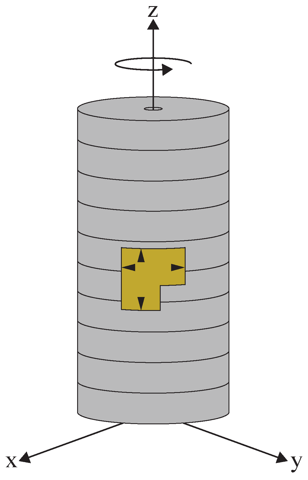
Geometry of a 0° specimen assuming TI symmetry featuring a biaxial strain gauge with triangles indicating measurement directions.
Figure 3.
Geometry of a 0° specimen assuming TI symmetry featuring a biaxial strain gauge with triangles indicating measurement directions.

Figure 4.
Examples of PT measured P- (red) and S-waveform (blue) amplitudes R (thick) and (thin) versus time t, respectively. Arrows indicate first arrivals.
Figure 4.
Examples of PT measured P- (red) and S-waveform (blue) amplitudes R (thick) and (thin) versus time t, respectively. Arrows indicate first arrivals.

Figure 5.
Confining pressure , pore pressure , and axial stress versus time t. Roman numbering combined with the grayscale background indicates the respective phases of fluid exposure: Phase (i), Phase (ii), and Phase (iii).
Figure 5.
Confining pressure , pore pressure , and axial stress versus time t. Roman numbering combined with the grayscale background indicates the respective phases of fluid exposure: Phase (i), Phase (ii), and Phase (iii).

Figure 6.
Schematics of the CO2 flow loop system that was used during the experiment under triaxial conditions. Modified from Agofack et al. [45].
Figure 6.
Schematics of the CO2 flow loop system that was used during the experiment under triaxial conditions. Modified from Agofack et al. [45].

Figure 7.
Axial strain versus time t. Roman numbering combined with the grayscale background indicates the respective phases of fluid exposure: Phase (i), Phase (ii), and Phase (iii).
Figure 7.
Axial strain versus time t. Roman numbering combined with the grayscale background indicates the respective phases of fluid exposure: Phase (i), Phase (ii), and Phase (iii).

Figure 8.
FO measured Young’s modulus (EV and its averaged namesake ) and Poisson’s ratio (vVH and its averaged namesake ) versus time t at 25 Hz. Roman numbering combined with the grayscale background indicates the respective phases of fluid exposure: Phase (i), Phase (ii), and Phase (iii). Rectangles in (a) indicate x- and y-limits in (b). Fifty measurements were averaged.

Figure 9.
PT measured P-wave velocity (VP0 and its averaged namesake ) and S-wave velocity (VP0 and its averaged namesake ) versus time t at 500 kHz. Roman numbering combined with the grayscale background indicates the respective phases of fluid exposure: Phase (i), Phase (ii), and Phase (iii). Rectangles in (a) indicate x- and y-limits in (b). Rectangles in (a) indicate x- and y-limits in (b). Ten measurements were averaged.

Figure 10.
FO measured Young’s modulus EV (a) and Poisson’s ratio vVH (b) versus frequency f with their respective regression lines at 43, 64, and 570 h corresponding to DT#1, DT#2, and DT#3.
Figure 10.
FO measured Young’s modulus EV (a) and Poisson’s ratio vVH (b) versus frequency f with their respective regression lines at 43, 64, and 570 h corresponding to DT#1, DT#2, and DT#3.

Figure 11.
Young’s moduli (, , and ), Poisson’s ratios (, , and ), stiffnesses (, , , , and ), and P- and S-wave velocities (, , , , and ) versus frequency f. Circles are measurements. Solid (dispersion) and dashed (attenuation) are modeled.
Figure 11.
Young’s moduli (, , and ), Poisson’s ratios (, , and ), stiffnesses (, , , , and ), and P- and S-wave velocities (, , , , and ) versus frequency f. Circles are measurements. Solid (dispersion) and dashed (attenuation) are modeled.


Table 1.
Mineralogical composition of Draupne Shale from X-ray diffraction (XRD) analysis.
| Mineralogy | Content (wt.%) |
|---|---|
| Quartz | |
| K-Feldspar | |
| Plagioclase | |
| Chlorite | |
| Kaolinite | |
| Mica-Illite | |
| Calcite | |
| Illite-Smcetite | |
| Siderite | |
| Dolomite | |
| Pyrite |
Table 2.
Physical properties of Draupne Shale provided by Skurtveit et al. [37] and SINTEF.
Table 2.
Physical properties of Draupne Shale provided by Skurtveit et al. [37] and SINTEF.
| Parameter(s) | Units | Values |
|---|---|---|
| Porosity | % | |
| Permeability | nD | |
| Grain density | g/cc | |
| Pore throat size | nm | |
| Pore fluid composition | % NaCl | |
| Water content | % |
Publisher’s Note: MDPI stays neutral with regard to jurisdictional claims in published maps and institutional affiliations. |
© 2021 by the authors. Licensee MDPI, Basel, Switzerland. This article is an open access article distributed under the terms and conditions of the Creative Commons Attribution (CC BY) license (https://creativecommons.org/licenses/by/4.0/).
Share and Cite
MDPI and ACS Style
Rørheim, S.; Bhuiyan, M.H.; Bauer, A.; Cerasi, P.R. On the Effect of CO2 on Seismic and Ultrasonic Properties: A Novel Shale Experiment. Energies 2021, 14, 5007. https://0-doi-org.brum.beds.ac.uk/10.3390/en14165007
AMA Style
Rørheim S, Bhuiyan MH, Bauer A, Cerasi PR. On the Effect of CO2 on Seismic and Ultrasonic Properties: A Novel Shale Experiment. Energies. 2021; 14(16):5007. https://0-doi-org.brum.beds.ac.uk/10.3390/en14165007
Chicago/Turabian StyleRørheim, Stian, Mohammad Hossain Bhuiyan, Andreas Bauer, and Pierre Rolf Cerasi. 2021. "On the Effect of CO2 on Seismic and Ultrasonic Properties: A Novel Shale Experiment" Energies 14, no. 16: 5007. https://0-doi-org.brum.beds.ac.uk/10.3390/en14165007
Note that from the first issue of 2016, this journal uses article numbers instead of page numbers. See further details here.