
Adaptive Cost Function FCSMPC for 6-Phase IMs


1
Systems Engineering and Automation Department, University of Seville, 41092 Seville, Spain
2
Electronic Engineering Department, University of Seville, 41092 Seville, Spain
*
Author to whom correspondence should be addressed.
Energies 2021, 14(17), 5222; https://0-doi-org.brum.beds.ac.uk/10.3390/en14175222
Submission received: 19 July 2021
/
Revised: 11 August 2021
/
Accepted: 19 August 2021
/
Published: 24 August 2021
(This article belongs to the Special Issue Control, Operation and Protection of Multiphase Machines and Drives)
Abstract
:In this paper, an adaptive cost function FCSMPC is derived from newly obtained results concerning the distribution of figures of merits used for the assessment of stator current model-based control of multi-phase induction machines. A parameter analysis of FCSMPC is carried out for the case of a six-phase motor. After extensive simulation and Pareto screening, a new structure has been discovered linking several figures of merit. This structure provides an simple explanation for previously reported results concerning the difficulty of cost function tuning for FCSMPC. In addition, the newly discovered link among figures of merit provides valuable insight that can be used for control design. As an application, a new cost function design scheme is derived and tested. This new method avoids the usual and cumbersome procedure of testing many different controller parameters.
1. Introduction
Multi-phase systems are preferred in some applications due to lower torque oscillations and harmonic content compared with conventional systems. Model-based control has found a new niche in multi-phase drives, under different schemes. Among them, Finite Control Set Model Predictive Control (FCSMPC) for stator current tracking is a popular one. In FCSMPC current control stator current control is the objective, whereas additional controllers are needed for flux and speed regulation [1]. The model-based controller computes the best Voltage Source Inverter (VSI) state by minimizing a function referred to as cost function.
The multi-phase VSI holds more configurations (switching states) than three-phase ones. Usually, a decomposition into () and () subspaces is considered to ease control design as these subspaces are related to different output variables such as torque production and losses [2].
In addition to current tracking and current rejection, the FCSMPC for current control can accommodate other objectives by an appropriate choice of the objective function. For multi-phase IM, arguably the most sought-after trait is that of low switching frequency. Such trait is, however, not easy to acquire as the tuning of the objective function is not trivial [3].
In this paper and continuing with the seminal work of [4], a selected number of variables for assessment (performance criteria) is used. The locus of these variables for different tunings of the FCSMPC reveals a not previously reported structure that links them. This finding means that a certain conservation law is in place, preventing the control system from simultaneously improving more than one performance criteria. This has implications for cost function design as will be discussed later. The methodology followed in the paper is to produce a large number of experimental values for the performance criteria obtained from different FCSMPC tunings; then, the data is fitted to a relatively simple mathematical expression. This structure provides an simple explanation for reported results. In addition, the newly discovered links among figures of merit provides valuable insight for the task of control design. An asymmetrical six-phase drive is considered for this study although the analysis can be carried out for other topologies.
The next section provides a background on previous works that are related to this one. In Section 3, the FCSMPC for current control is summarized to provide the basis for the analysis of the figures of merit. The newly discovered link between figures of merit is presented in Section 4, where Pareto analysis and cubic titeica approximation are shown. The discovery is then applied, in Section 5, to derive a new FCSMPC cost function design scheme that is experimentally tested.
2. Related Works
Control systems assessment is an important part of the engineering practice; however, it seldom appears in most journals. In the case of FCSMPC for the broader field of electric machines, assessment is reduced to a few operating points and a parameter analysis is seldom performed. For instance, ref. [5] presents the surfaces of some figures of merit for a distribution of operating points covering the speed and load range. Similarly, refs. [1,6] presents a large set laboratory and simulated experiments enabling the assessment of the FCSMPC using a five-phase IM. In [7], four current controllers for the six-phase IM are thoroughly compared using the Root Mean Squared (RMS) value of tracking error and Total Harmonic Distortion (THD) of the stator currents as performance indices. More recently, ref. [8] presents an analysis of predictive current control for six-phase IM with alternate winding configurations.
Another related topic is that of cost function design for FCSMPC systems. This topic is mainly concerned with finding adequate cost function parameters so that the closed-loop IM behavior meets requirements. This task is not easy as the cost function parameters affect every aspect of the IM behavior. In particular, the design for current controllers must face conflicting objectives. As an example consider that tracking in leads to some content due to the use of voltage vectors with projection. Of course, a high content is undesirable as copper losses increase. But, on the other hand, a poor tracking can produce speed ripple. This has been studied in the seminal paper [4] where trade-offs are discussed and recently in [9] where Pareto analysis is used.
Instead of the cumbersome trial and error process, usually found in the above cited works, other methods have been proposed such as neural approximations, changes in the cost function to avoid weighting factors and replacement of the cost function by decision making schemes such as fuzzy inference. For instance, in [2] an automated method is used to select the weights of the cost function for the control of a Shunt Filter of Active Power. In [3] the MPC formulation is used to include soft constraints for a nine-phase IM drive and the effect of cost function parameters is discussed. In [10] a fuzzy adaptive speed controller and adaptive weighting factors are used to reduce the speed, torque and flux ripples. Other proposals can be found in the review of [11].
Regarding weighting factor elimination, in [12] a predictive direct torque control without cost function weighting factors is presented. A multi-objective ranking is used to decide the voltage vector to be applied from a limited set. AS a result the switching frequency and computational effort can be ameliorated. In a different approach, ref. [13] presents a dynamic virtual voltage vectors strategy designed to attain zero (on average) voltage production; as a result the MPC cost function can be simplified and the parameter eliminated. In this paper the opposite approach is taken following the hypothesis that cost function parameters provide some flexibility that is lost otherwise.
3. Predictive Current Control of Multi-Phase IM
Multi-phase IM speed regulation can be done using a classical control loop. For the stator current control, accurate tracking of components and rejection of currents are needed. The electro-mechanical power conversion is due solely to components. The plane does not contribute to torque and its components must be minimized.
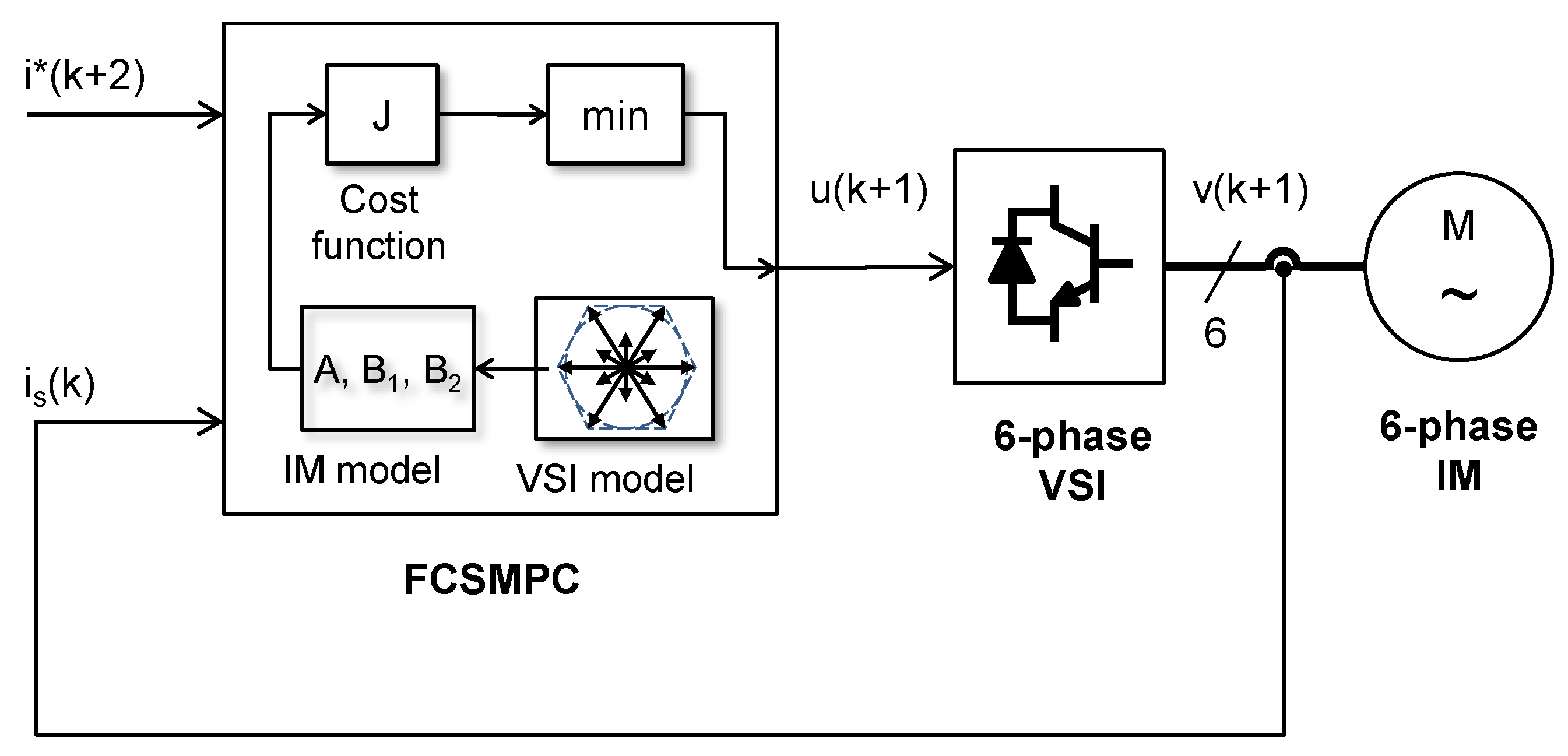
Figure 1 illustrates FCSMPC for stator current of a six-phase motor. It works by providing the control signal u that sets the state of the VSI for a whole sampling period. This is done computing, at discrete time k, the optimal switch configuration for the period. The voltage is impressed on the IM with the objective of producing currents following a reference trajectory .
The objective function considers predictions for since will not affect the measurements made until that time. The predictions are supplied by a mathematical model of the drive which is derived from the IM equations. After some manipulation, the predictive model takes the form
In (1), , and result from discretization of the continuous time dynamics [1]. The actual angular speed must be measured along with the components of the state space vector . Also, in (1) the quantity is due to rotor currents (unmeasurable in most cases). This term is thus estimated using a backtracking method [1] as follows
In the above equations, is the sampling time and is a vector of VSI switch states .
The actual control action is computed at discrete time k minimizing a cost function J. In this paper J is made up of terms corresponding to the penalization of tracking errors in , rejection of components and a term penalizing the number of switch changes in the VSI. This number is computed as
Then the objective function can be expressed as
where is the quadratic deviation of predictions from reference in plane and is the quadratic deviation of predictions from reference in plane. The temporal index k has been omitted for clarity.
3.1. Cost Function Tuning
Combining previous Equations (1)–(4) it is possible to derive as the VSI state that minimizes J. In FCSMPC and related approaches this is usually done by exhaustive (or restrained) exploration of the possible VSI states.
In this scenario, tuning of the FCSMPC consists on selecting the values for parameters and . This is usually done by trial and error, having as guidance some performance indices or figures of merit as the ones presented later on in the paper.
The problem of cost function tuning (selection of cost functions weights) has appeared in the literature associated with stator current control of multi-phase machines, but it also appears in connection with Predictive Torque Control and in other applications where conflicting criteria must be dealt with. In fact, it has received considerable attention in recent works. The approach taken in this paper is that cost function tuning dictates the future behavior of the IM drive. Figures of merit are usually used, in the broader context of automatic control and also in the particular case of FCSMPC, to quantify such behavior in a useful way. Having this in mind, the problem of cost function tuning is viewed as the selection of weights to produce adequate figures of merit or performance indices such as the ones presented in the following.
3.2. Performance Indices
Controllers for drives can be assessed by different figures of merit such as harmonic content [14,15,16], speed of response [17], steady state torque ripple [18,19], current imbalance [20], commutation losses [21,22], and total losses [23]. Of course these figures of merit are not independent. Consider as an example the usual case of sinusoidal references for stator currents. The quality of tracking is then inversely proportional to Total Harmonic Distortion (THD) so both quantities are somehow linked. Another example is current content in the being linked to copper losses and current THD. Oscillations in drive speed are produced by ripples in torque that are produced by imperfect tracking in plane. Finally, average switching frequency is larger for tunings where current tracking requirements are more stringent, so better tracking usually requires more commutations.
Continuing with the work [4], three measures (, and ) will be used as they are directly related to most of the issues above presented. Their values are computed from experiments where references for are sinusoidal and zero for . After the experiment is performed, data from N sampling periods is used to compute the values as follows
From the definition it is clear that is the RMS value of the stator current tracking error in . From the considerations made above, this value is directly related to stator current THD and to torque ripple, so, a low provides not only better tracking, but also less THD and less torque ripple. Similarly, is the RMS value of the stator current tracking error in plane and is related to THD and copper losses. Clearly, the lower the better from an energy efficiency stand-point. Finally, is the average commutation frequency for the VSI. Please notice that in FCSMPC there is not fixed commutation rate, so one must rely on averaged values such as . This commutation frequency must be kept low due to VSI limits and due to energy efficiency considerations as commutation losses are related to this quantity.
In any application one can think of, the FCSMPC designer would try to minimize all , and . A good predictive model and low sampling period are key factors to achieve this objective. This route has been explored in many papers dealing with identification [6,24,25], different kinds of models (including models with observers) and schemes for diminishing the application period such as in-sample or space-vector modulation [5,26,27,28] and virtual voltage modulation [13,29].
Tuning of the cost function J also plays a crucial role in the observed values of the indices. This paper analyzes the links between the values when and are varied over a wide range of values. The distribution of values shows a remarkable pattern never reported before that links the three figures of merit. As an application, the paper also proposes an adaptive scheme for automatic cost function tuning.
3.3. Six-Phase Drive
The multi-phase IM used in this paper is a motor with two three-phase sets of windings in an asymmetrical configuration. Two three-phase VSI connected as depicted in Figure 2 are used to supply voltage to the motor.
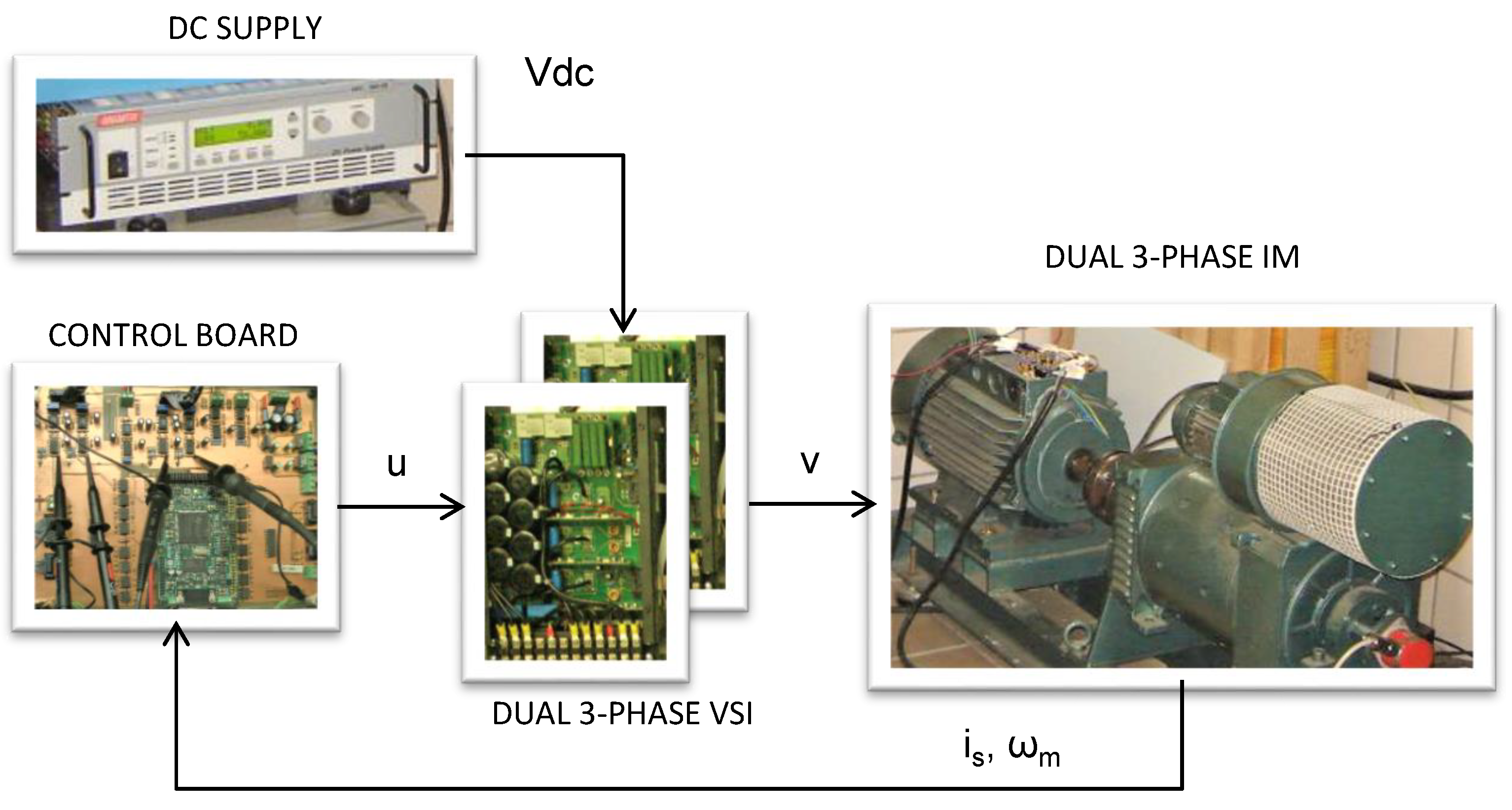
Table 1 presents the main data from the name-plate and the identified parameters for the motor. The VSI are SKS21F (Semikron) inverters commanded using the TMS320F28335 Texas Instruments DSP on a MSK28335 board. Two neutral points are used and the stator currents measured with four hall-effect sensors. The speed is measured using quadrature encoders. Load can be applied independently thanks to a DC-motor sharing the shaft. Figure 3 depicts the main components of the experimental setup.
4. Cubic Titeica Approximation
The aim of this section is showing that the already reported links among figures of merit (the values) follow a simple formula that has been experimentally derived. This discovery is by itself interesting as it show that some sort of conservation law is in place, meaning that it is impossible to obtain better results in terms of without altering the other two figures of merit and . This is important as in any application one can think of, all three indices are important, so a compromise or trade-off solution must be sought. In this section, the procedure followed for data-gathering and processing will be presented, this will lead to the discovery that the values lie in a surface and thus are tied to one another. The particular surface will be identified leading the way for an application for FCSMPC design.
4.1. Data Gathering
The first step for the analysis is collecting data from the operation of the 6-phase motor driven by the FCSMPC in current control mode. For the analysis, thousands of data points have to be collected corresponding to various tunings of the cost function (i.e., to different combinations of . To do so, an adequate model must be derived to be used in simulation. Sinusoidal excitation methods have been used to identify the parameters of the IM [24]. A Runge-Kutta method for the numerical integration of the continuous-time differential equations has then be deployed. In the simulations, the controller runs at (s) and it is treated as a discrete-time subsystem. The reference signal for stator current traking uses an amplitude (A) and a frequency (Hz); thus
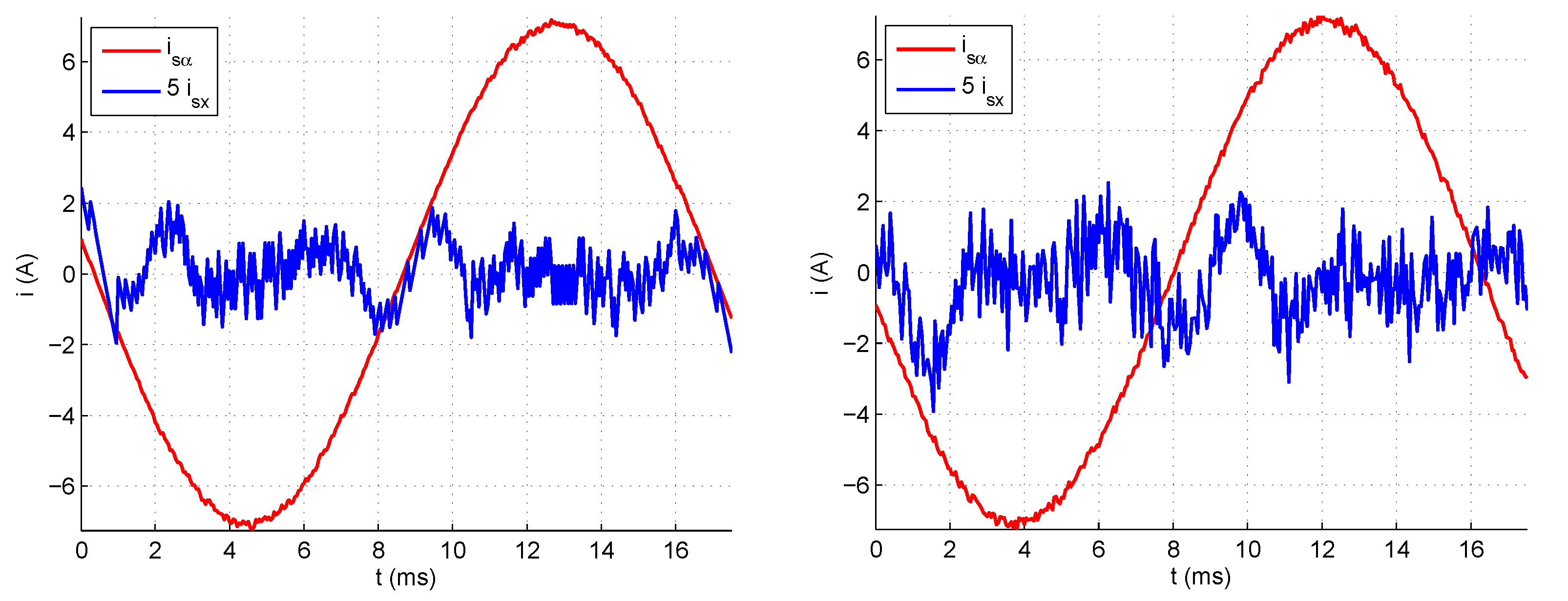
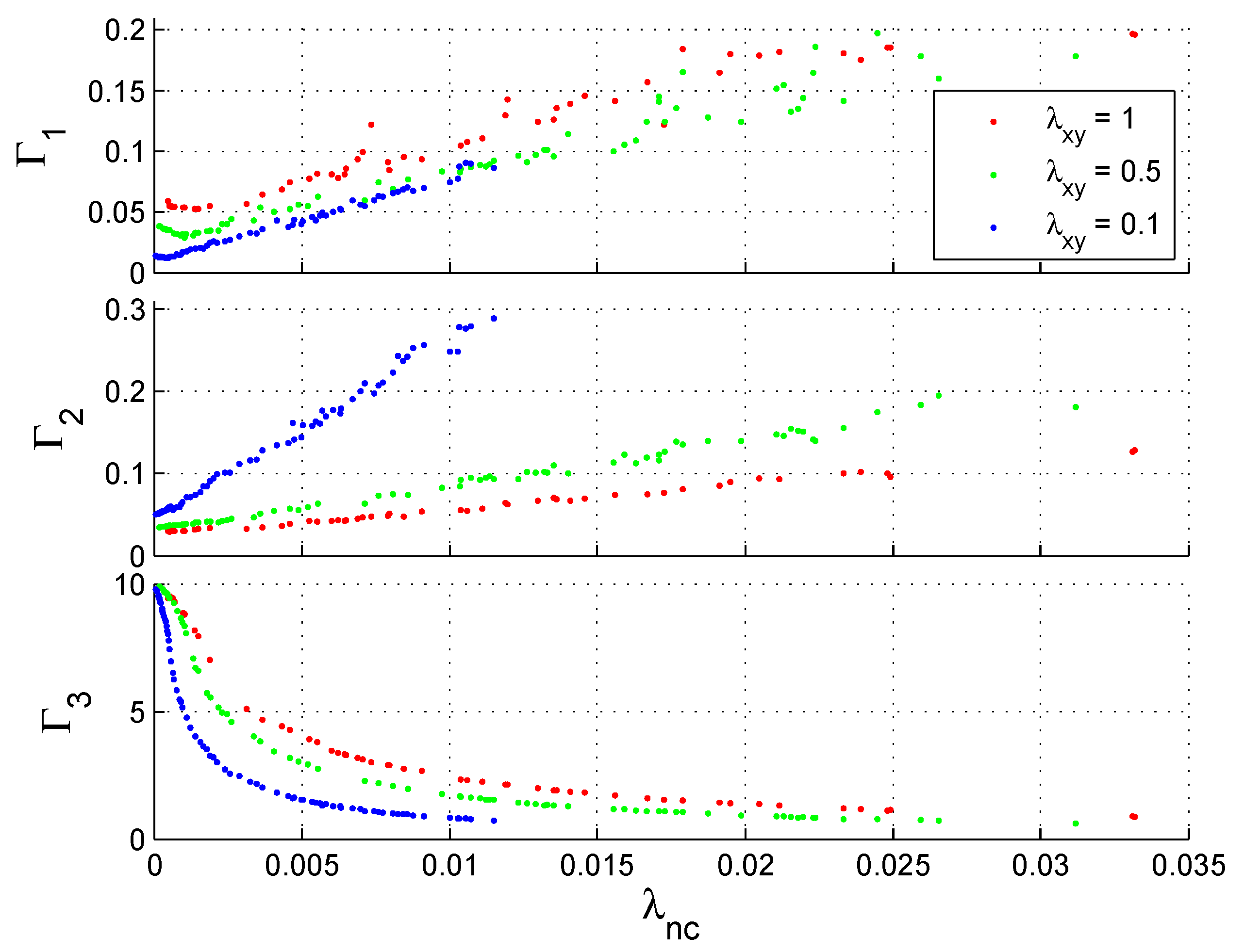
For each the simulation is run for a number of sampling periods N including some electrical cycles enough to compute the quantities to as averages according to their definition. The fit of the simulations to actual measurements has been checked using the figures of merit as shown in [4]. Figure 4 shows the experimental waveforms for two choices of . Notice that the vertical axis for the curve has been scaled to provide a 5× zoom for readability. It can be seen that the effect of increasing is noticeable in stator current tracking, mainly (for this particular example) in components. This kind of representation is useful to compare few cases and to gain insight into the problem. However, to advance in the analysis one needs to resort to some quantification as provided by the indices. Then new information arises, as shown in Figure 5, that will be discussed later.
4.2. Pareto Optimality
The values found for a combination might have different merits for different applications. It is clear, however, that the lower their value, the better. What one finds in many cases is that, for some tunings, one of the values decreases at the expense of an increase in the other two.
The concept of Pareto optimality allows us to derive a reduced set of combinations that are of interest for design in many fields. Recall that a combination is deemed Pareto-optimal if it is not dominated by other combination. A combination is said to be dominated by if for all i and for a particular m, holds. These conditions indicate that is at least as good as regarding all of their indices i, and at least for some index (m) the combination is actually better.
The Pareto frontier is the set of all combinations that are Pareto-optimal (i.e., not dominated). In this paper, Pareto-optimality has been used to exclude combinations that are not optimal regardless of the application. From a set of 4923 combinations of just 1415 turned out to be on the Pareto frontier. This screening not only reduces the number of data points to be considered but also allow for a more focused search for links among figures of merit.
4.3. Data Surface
The relationship between and is not straightforward. It must be noted that the controller aims to minimize the cost function that includes three terms that are related to the three components of ; however, the point to point minimization of J (4) does not imply a similar minimization of the three components of . This can be checked in Figure 5, where the various performance indices found in the simulations are plotted against some of the combinations used in said simulations. Some general tendencies can be seen, but not much more; in fact, the data points seem to follow intricate paths. A low order approximation (e.g., linear, quadratic) seems useless. Please note that there are gaps in the distribution. This is due to the pruning of data points performed by the Pareto screening. In particular, the line of points for ends abruptly at around , this is not a mistake, is just a reflection of the fact that not all tunings yield Pareto-optimal results.
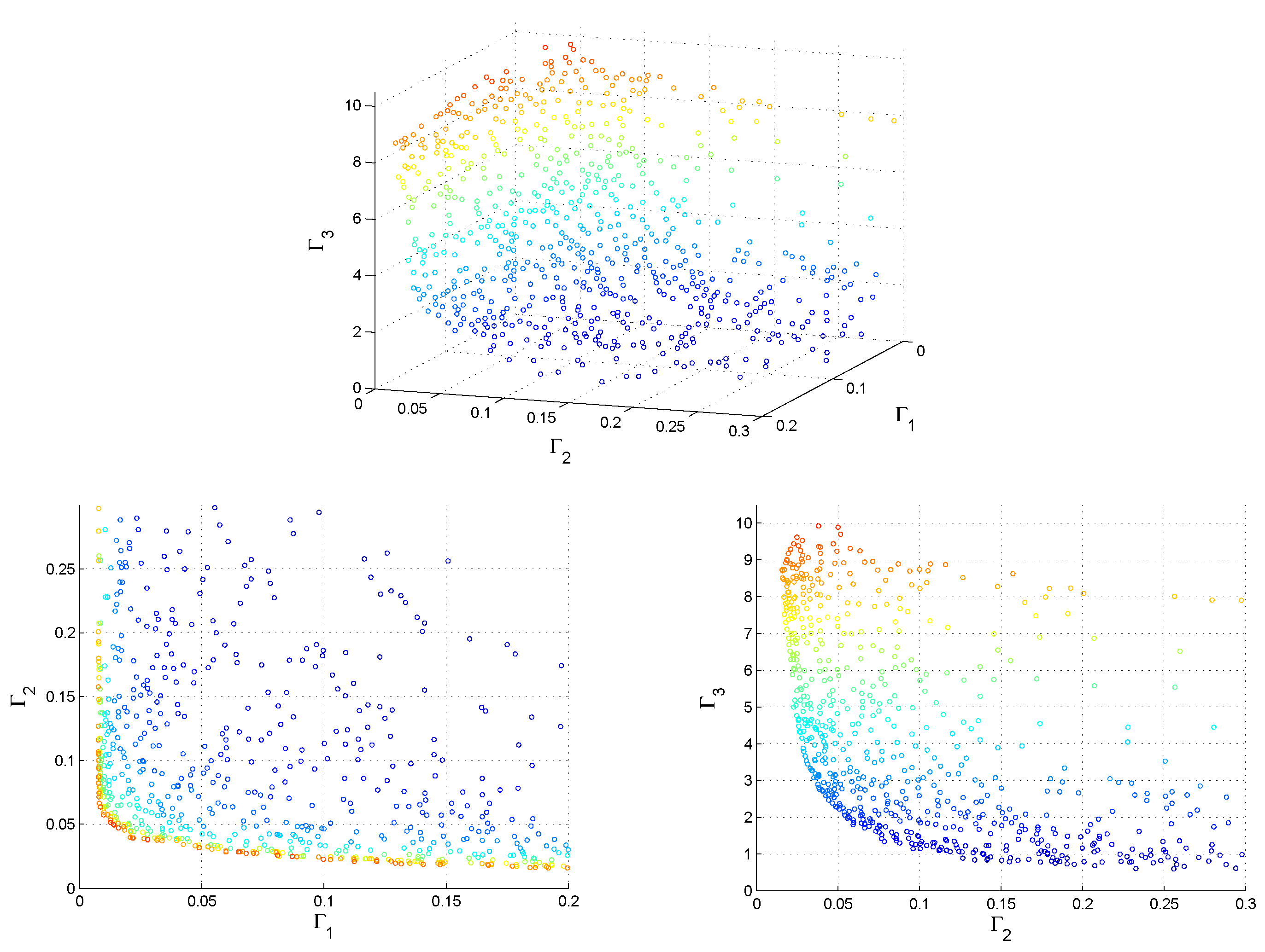
On closer inspection, the 3D distribution of the values seem to fit a smooth surface as shown in Figure 6. A total of 671 points have been chosen from the Pareto optimal set in order to provide a graphical representation that is not too dense or too sparse. The points are represented with marks with a different color for each value of , in this way it is easier to relate points in the projections. It can be seen that the distribution seems to be asymptotic for large values of , indicating a 3D generalization of the hyperbola. Such generalization has the amazingly simple expression
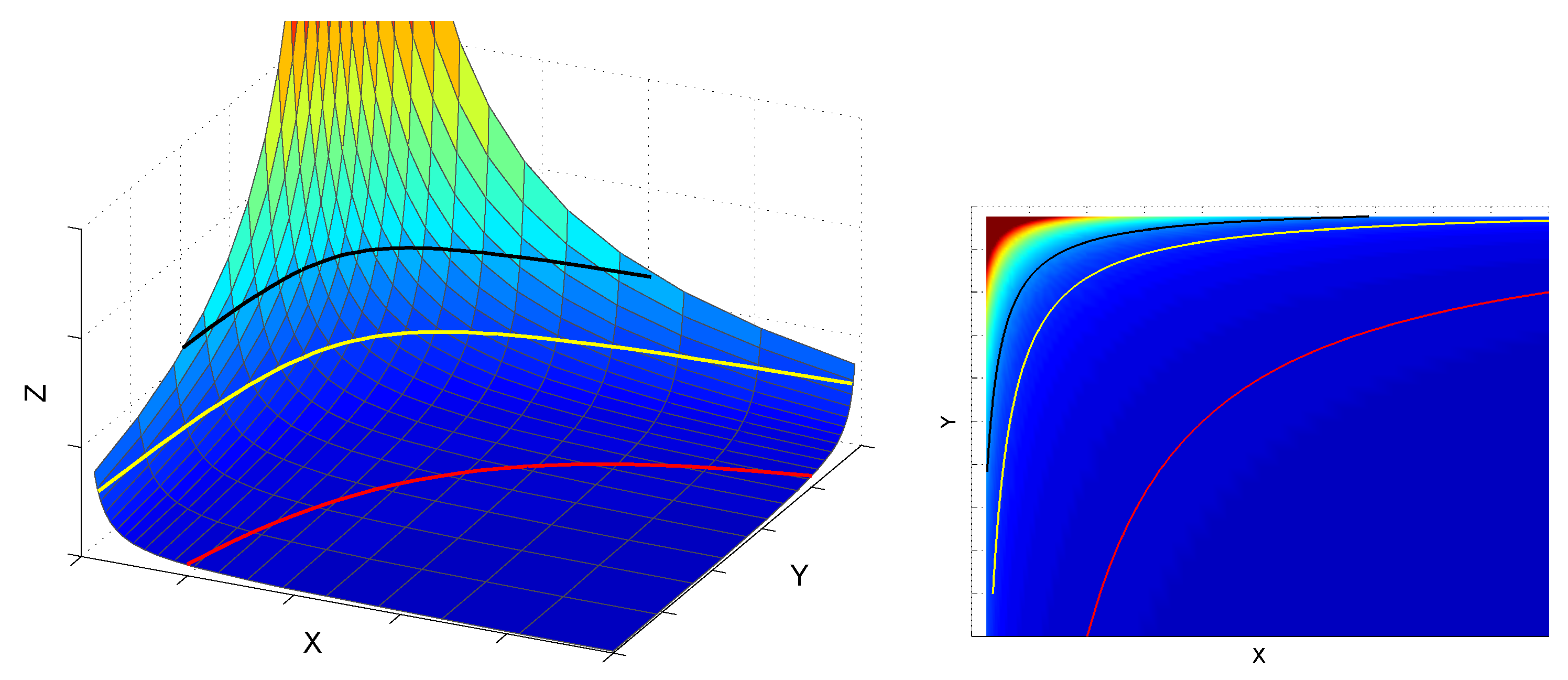
where represent the coordinates of a point in 3D space and K denotes a constant. The cubic Equation (9) yields a titeica surface studied by G. Tzitzéica [30]. Figure 7 presents the titeica surface; several cuts have been performed by horizontal planes for some showing the resulting hyperbolas of the form .
It is possible to fit the values to the model (9) by allowing some translation of the axis. Thus, if one takes , , and then the observed value for K is obtained for . This is a remarkable finding as it links the performance indices to one another via a simple expression.
This clearly shows that it is impossible to improve one index without degrading at least one of the other two. Further implications will be discussed later.
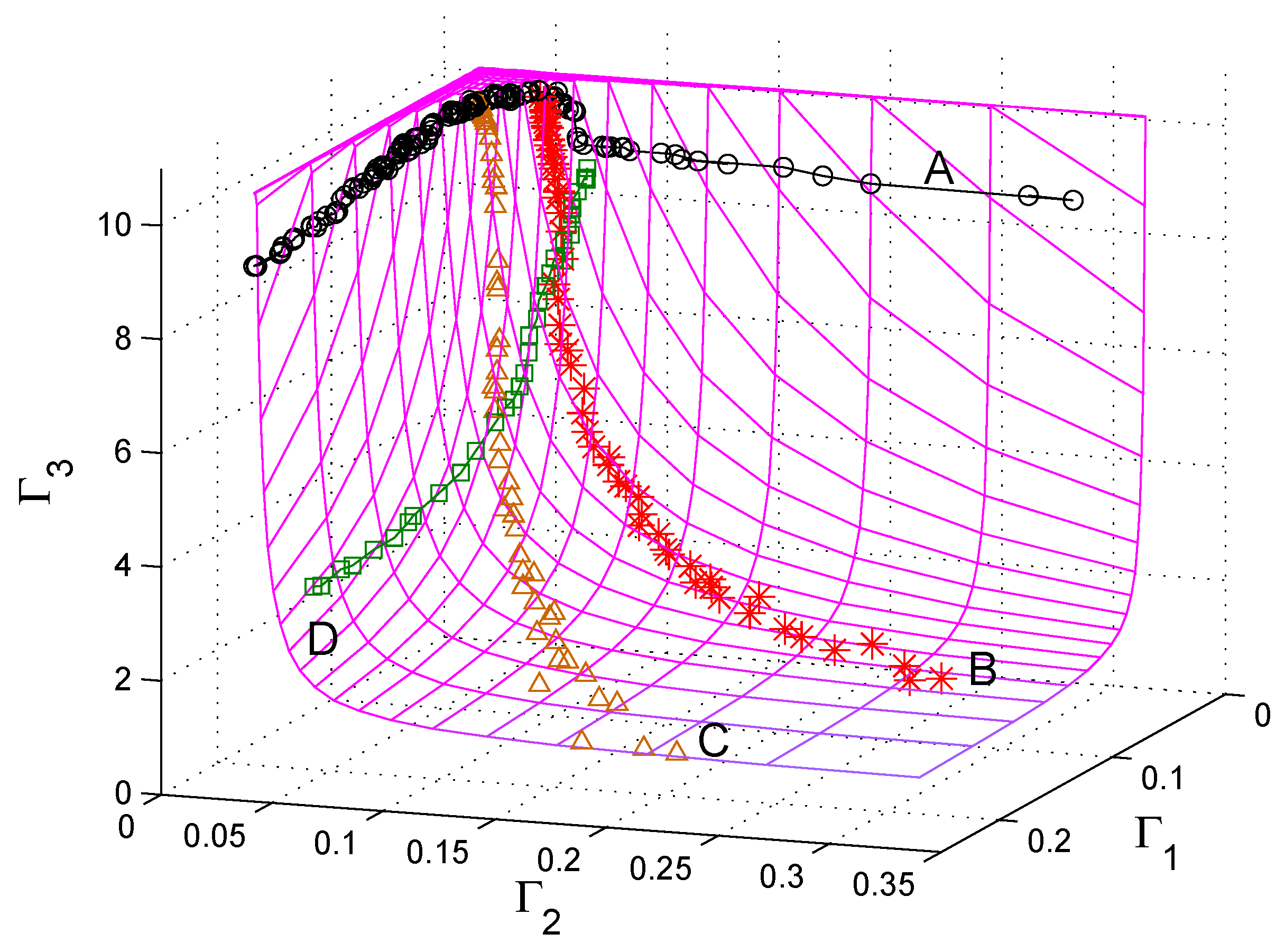
Figure 8 shows the titeica surface fitted to data represented by Equation (10). Please notice that the upper part of the surface has been trimmed for ease of presentation. In addition, some values are presented to further study the distribution. These values are commented in the following.
- Line A is made up of values from simulations where . The values gather close to a line placed on the surface in the upper region. In fact this line is the upper limit of . The line is not an hyperbola (although its general shape resembles one, specially viewed from above) as it contains some wiggles or bumps specially for low values of . increases from right to left producing increasing values of and decreasing values of according to (10).
- Line B corresponds to tunings where . The value of goes from at the intersection with line A to a value of near the bottom. The switching frequency goes down as both increase.
- Line C corresponds to tunings where . The line found is similar to that of the previous case. Please note that both and have been proposed in the literature combined with low values of . This tuning produces values that are close to the Z axis, meaning that have both a low value even with a decrease in as the surface is very steep at that region. These two choices are adequate in cases where current tracking is the main concern leaving little allowance for lowering losses.
- Line D, finally, is made up of values from simulations where . The line is almost parallel to the XZ plane. It provides tunings where changes little at the expense of pronounced changes in the other two indices.
The cases commented above are easy to implement as they just require selecting values of the design parameters and . These cases provide insight into the cubic surface and the underlying relationship of Equation (10). In particular, they show that the relationship between and is far from trivial.
5. Application to FCSMPC Design
The above results highlight two aspects that difficult FCSMPC design for multi-phase IM: (1) cost function parameters have not a straightforward link to figures of merit and (2) figures of merit are not free to take any combination.
In the following, a novel scheme for FCSMPC design is presented. A commonplace scenario is chosen to illustrate the procedure but the method can be applied to other situations. In many applications the main concern is that of performance with losses being a secondary objective. Losses are linked to high values of , whereas performance is achieved with low values of . Then, for this scenario, it makes sense to design the FCSMPC cost function as the solution to the following optimization problem:
where is the maximum value of that one is willing to accept and, similarly, is the maximum value for .
The optimization of (11) is still a time-consuming task, so it seems that nothing has been gained. However, from the first constraint it is clear that minimization of means taking the extreme values for the other two figures of merit, that is: and . Still it is not clear how to derive the value for . An observation can be made here, the tuning with will most likely produce the smallest value of but producing large values for the other two figures of merit. Now, the MIT rule can be used to set up an adaptive scheme where the values will evolve until the conditions , are met.
It is well known that the MIT rule requires the derivatives of the error to be computed. A simplified version has been used sometimes to avoid such computation, the derivatives are substituted by average values. Then the values can be updated in the following way
where , are adaptation gains that affect the convergence speed.
5.1. Implementation Details
It is important to notice that (12) and (13) require measurement of , . But these values are computed as averaged measures over a temporal horizon. This means that the adaptation should not be run at the same speed as the FCSMPC. This is not much of a drawback for two reasons: first, in adaptive systems the adaptation is in most cases slow to avoid instability issues due to the coupling of dynamics; second, the time required for adaptation is still low compared with the mechanical time constant for much applications (except perhaps for ultra-fast tiny motors).
In addition, note that the initial value taken for the FCSMPC parameter vector is not special and can be replaced with other values. The only particular consideration is that should make the IM run, even with higher losses.
The amount of extra computations needed for the implementation of the adaptive procedure is low if it is carried out by averaging quantities for each sampling time k in accordance with (5)–(7). Then a particular sampling period can be devoted to update . The procedure is then repeated.
With this in mind, the parameter adaptation can be done every N sampling periods as
where the arrow operator is to be realized as an assignment in the particular programming language of the DSP.
5.2. Experimental Results
The FCSMPC scheme with cost function (4) has been modified to include adaptation of parameters every sampling periods (0.025 s) according to (14) and (15). The adaptation gains have been set to and .
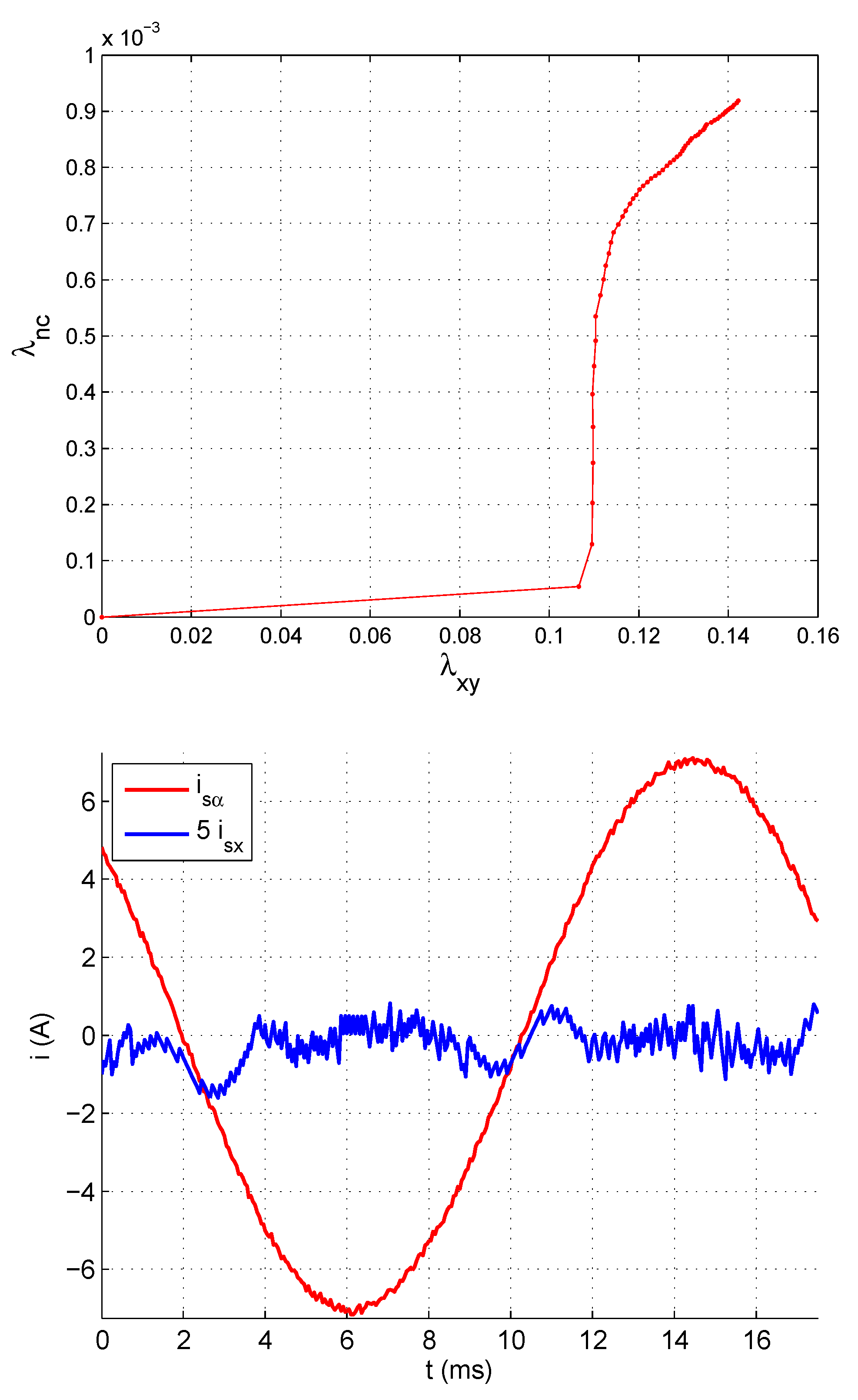
Figure 9 (top graph) shows the results obtained for the adaptation. The initial value is (lower left) yielding which does not comply with the specifications. As the adaptation progresses, the parameters change values, first more steeply because of the larger value of the error , and later on more slowly as is the usual case with gradient-based schemes such as the MIT rule.
It can be seen that the sequence converges to 9 × 10. After 20 adaptation steps (0.5 s), the figures of merit take values that are already close enough to the design values. It can be seen that performance is guaranteed by the relatively low value of whereas the other figures of merit lie in their specified region.
The lower part of Figure 9 shows the waveforms for stator currents in and x axis for the final values of the adapted parameters. Similar results are obtained for and x and are omitted for brevity. The adequacy of the tuning can be checked by visual inspection.
6. Discussion
The problem of cost function design for FCSMPC of multi-phase IM has been tackled taking a six-phase motor as an example.
The Pareto analysis of the figures of merit and posterior fitting to a cubic titeica surface has resulted in the, not previously reported, mathematical expression of (10). This expression allows a simple explanation of the complex behavior found in previously reported results. In particular, the often-mentioned tedious task of cost function tuning is clearly shown to be a difficult problem. But perhaps the most striking result is the simple formula found for the figures of merit (8). This experimentally-derived expression clearly shows that, once in the Pareto frontier, improving one figure of merit must come in detriment of the other two in a drastic way as indicated by the hyperbolic inverse law embedded in (8).
The Pareto analysis and the cubic titeica approximation also provide support for developing new techniques. As an example, an adaptive method for the tuning of FCSMPC cost function parameters has been presented. With this approach, the problem of cost function design no longer imply the cumbersome trial and error process of past approaches. Also, thanks to the analysis performed previously, optimality (with respect to the figures of merit) is taken care of. The experiments and analysis of the proposed adaptive cost function show its feasibility and flexibility to accommodate different design criteria. In particular the case in which one is mainly concerned with performance (provided by accurate tracking) and a bit less by energy efficiency ( content and commutations) has been used as an example. The experimental waveforms confirm the validity of the proposed scheme and its adaptation law.
Author Contributions
Methodology/Conceptualization M.R.A. and F.B.; software, M.G.S.; validation, M.R.A., M.G.O. and M.G.S.; formal analysis, investigation, resources and data curation M.R.A. and M.G.S.; writing, review, editing, and visualization, M.R.A., M.G.O. and F.B.; supervision, project administration and funding acquisition, M.G.O. and M.R.A. All authors have read and agreed to the published version of the manuscript.
Funding
The current research has been funded with grant Proyecto RTI2018-101897-B-I00 by FEDER/Ministerio de Ciencia e Innovación—Agencia Estatal de Investigación. Spain.
Conflicts of Interest
The authors declare no conflict of interest.
Abbreviations
| IM variables | |
| i | Current |
| v | Voltage |
| Angular speed | |
| Electrical frequency | |
| Subscripts | |
| Subspace for energy conversion | |
| Subspace not related to energy conversion | |
| Superscripts | |
| * | Reference |
| Prediction or estimated value | |
| Control parameters and variables | |
| J | Cost function |
| Weighting factor penalizing currents | |
| Weighting factor penalizing commutations | |
| Vector of FCSMPC parameters | |
| Vector containing figures of merit | |
| Sampling period | |
References
- Martín, C.; Bermúdez, M.; Barrero, F.; Arahal, M.R.; Kestelyn, X.; Durán, M.J. Sensitivity of predictive controllers to parameter variation in five-phase induction motor drives. Control Eng. Pract. 2017, 68, 23–31. [Google Scholar] [CrossRef] [Green Version]
- Zanchetta, P. Heuristic multi-objective optimization for cost function weights selection in finite states model predictive control. In Proceedings of the 2011 Workshop on Predictive Control of Electrical Drives and Power Electronics (PRECEDE), Munich, Germany, 14–15 October 2011; pp. 70–75. [Google Scholar]
- Gonzalez-Prieto, I.; Zoric, I.; Duran, M.J.; Levi, E. Constrained model predictive control in nine-phase induction motor drives. IEEE Trans. Energy Convers. 2019, 34, 1881–1889. [Google Scholar] [CrossRef]
- Arahal, M.R.; Barrero, F.; Duran, M.J.; Ortega, M.G.; Martin, C. Trade-offs analysis in predictive current control of multi-phase induction machines. Control Eng. Pract. 2018, 81, 105–113. [Google Scholar] [CrossRef]
- Barrero, F.; Arahal, M.R.; Gregor, R.; Toral, S.; Durán, M.J. One-Step Modulation Predictive Current Control Method for the Asymmetrical Dual Three-Phase Induction Machine. Ind. Electron. IEEE Trans. 2009, 56, 1974–1983. [Google Scholar] [CrossRef]
- Lim, C.S.; Levi, E.; Jones, M.; Rahim, N.A.; Hew, W.P. FCS-MPC-based current control of a five-phase induction motor and its comparison with PI-PWM control. IEEE Trans. Ind. Electron. 2014, 61, 149–163. [Google Scholar] [CrossRef]
- González, O.; Ayala, M.; Romero, C.; Rodas, J.; Gregor, R.; Delorme, L.; González-Prieto, I.; Durán, M.J.; Rivera, M. Comparative Assessment of Model Predictive Current Control Strategies applied to Six-Phase Induction Machines. In Proceedings of the 2020 IEEE International Conference on Industrial Technology (ICIT), Buenos Aires, Argentina, 26–28 February 2020; pp. 1037–1043. [Google Scholar]
- Shawier, A.; Habib, A.; Mamdouh, M.; Abdel-Khalik, A.S.; Ahmed, K.H. Assessment of predictive current control of six-phase induction motor with different winding configurations. IEEE Access 2021, 9, 81125–81138. [Google Scholar] [CrossRef]
- Fretes, H.; Rodas, J.; Doval-Gandoy, J.; Gomez, V.; Gomez, N.; Novak, M.; Rodriguez, J.; Dragičević, T. Pareto Optimal Weighting Factor Design of Predictive Current Controller of a Six-Phase Induction Machine based on Particle Swarm Optimization Algorithm. IEEE J. Emerg. Sel. Top. Power Electron. 2021. [Google Scholar] [CrossRef]
- Zhang, Z.; Wei, H.; Zhang, W.; Jiang, J. Ripple Attenuation for Induction Motor Finite Control Set Model Predictive Torque Control Using Novel Fuzzy Adaptive Techniques. Processes 2021, 9, 710. [Google Scholar] [CrossRef]
- Mamdouh, M.; Abido, M.; Hamouz, Z. Weighting Factor Selection Techniques for Predictive Torque Control of Induction Motor Drives: A Comparison Study. Arab. J. Sci. Eng. 2018, 43, 433–445. [Google Scholar] [CrossRef]
- Ipoum-Ngome, P.G.; Mon-Nzongo, D.L.; Song-Manguelle, J.; Flesch, R.C.; Jin, T. Optimal finite state predictive direct torque control without weighting factors for motor drive applications. IET Power Electron. 2019, 12, 1434–1444. [Google Scholar] [CrossRef]
- Aciego, J.J.; Prieto, I.G.; Duran, M.J.; Bermudez, M.; Salas-Biedma, P. Model predictive control based on dynamic voltage vectors for six-phase induction machines. IEEE J. Emerg. Sel. Top. Power Electron. 2020, 9, 2710–2722. [Google Scholar] [CrossRef]
- Luo, Y.; Liu, C. A Simplified Model Predictive Control for a Dual Three-Phase PMSM Motor with Reduced Harmonic Currents. IEEE Trans. Ind. Electron. 2018, 65, 9079–9089. [Google Scholar] [CrossRef]
- Hachi, N.; Kouzou, A.; Hafaifa, A.; Iqbal, A. Application of the Model Predictive Control and the SVPWM Techniques on Five-phase Inverter. Electroteh. Electron. Autom. 2019, 67, 17–28. [Google Scholar]
- Kindl, V.; Cermak, R.; Ferkova, Z.; Skala, B. Review of time and space harmonics in multi-phase induction machine. Energies 2020, 13, 496. [Google Scholar] [CrossRef] [Green Version]
- Mohamed, Y.A.R.I.; El-Saadany, E.F. Robust high bandwidth discrete-time predictive current control with predictive internal model—A unified approach for voltage-source PWM converters. IEEE Trans. Power Electron. 2008, 23, 126–136. [Google Scholar] [CrossRef]
- Xia, C.; Wang, Y.; Shi, T. Implementation of finite-state model predictive control for commutation torque ripple minimization of permanent-magnet brushless DC motor. IEEE Trans. Ind. Electron. 2013, 60, 896–905. [Google Scholar] [CrossRef]
- Zhang, Y.; Yang, H.; Xia, B. Model predictive torque control of induction motor drives with reduced torque ripple. IET Electr. Power Appl. 2015, 9, 595–604. [Google Scholar] [CrossRef]
- Hu, Y.; Zhu, Z.Q.; Liu, K. Current control for dual three-phase permanent magnet synchronous motors accounting for current unbalance and harmonics. IEEE J. Emerg. Sel. Top. Power Electron. 2014, 2, 272–284. [Google Scholar]
- Preindl, M.; Schaltz, E.; Thogersen, P. Switching frequency reduction using model predictive direct current control for high-power voltage source inverters. IEEE Trans. Ind. Electron. 2011, 58, 2826–2835. [Google Scholar] [CrossRef]
- Li, Z.; Guo, Y.; Xia, J.; Li, H.; Zhang, X. Variable sampling frequency model predictive torque control for VSI-fed im drives without current sensors. IEEE J. Emerg. Sel. Top. Power Electron. 2020, 9, 1507–1517. [Google Scholar] [CrossRef]
- Rivas, J.J.R.; Montiel, J.P.; Badaoui, M.; Farias, J.M.A.; Castillo, O.C.; González, R.O. Optimization of the efficiency in an induction machine drive by algorithm based on the interior point method. Rev. Iberoam. Autom. Inform. Ind. 2021. [Google Scholar] [CrossRef]
- Yepes, A.G.; Riveros, J.A.; Doval-Gandoy, J.; Barrero, F.; López, O.; Bogado, B.; Jones, M.; Levi, E. Parameter identification of multiphase induction machines with distributed windings—Part 1: Sinusoidal excitation methods. IEEE Trans. Energy Convers. 2012, 27, 1056–1066. [Google Scholar] [CrossRef]
- Heydari, R.; Young, H.; Rafiee, Z.; Flores-Bahamonde, F.; Savaghebi, M.; Rodriguez, J. Model-Free Predictive Current Control of a Voltage Source Inverter based on Identification Algorithm. In Proceedings of the IECON 2020 The 46th Annual Conference of the IEEE Industrial Electronics Society, Singapore, 18–21 October 2020; pp. 3065–3070. [Google Scholar]
- Difi, D.; Halbaoui, K.; Boukhetala, D. Hybrid control of five-phase permanent magnet synchronous machine using space vector modulation. Turk. J. Electr. Eng. Comput. Sci. 2019, 27, 921–938. [Google Scholar] [CrossRef]
- Difi, D.; Halbaoui, K.; Boukhetala, D. High Efficiency and Quick Response of Torque Control for a Multi-Phase Machine Using Discrete/Continuous Approach: Application to Five-phase Permanent Magnet Synchronous Machine. System 2021, 1, 2. [Google Scholar]
- Song, Z.; Hu, S.; Bao, Z. Variable Action Period Predictive Flux Control Strategy for Permanent Magnet Synchronous Machines. IEEE Trans. Power Electron. 2019, 35, 6185–6197. [Google Scholar] [CrossRef]
- Yuan, Q.; Li, A.; Qian, J.; Xia, K. Dc-link capacitor voltage control for the NPC three-level inverter with a newly MPC-based virtual vector modulation. IET Power Electron. 2020, 13, 1093–1102. [Google Scholar] [CrossRef]
- Tzitzéica, M.G. Sur une nouvelle classe de surfaces. Rend. Circ. Mat. Palermo 1908, 25, 180–187. [Google Scholar] [CrossRef] [Green Version]
Figure 1.
Diagram of FCSMPC of a six-phase IM.

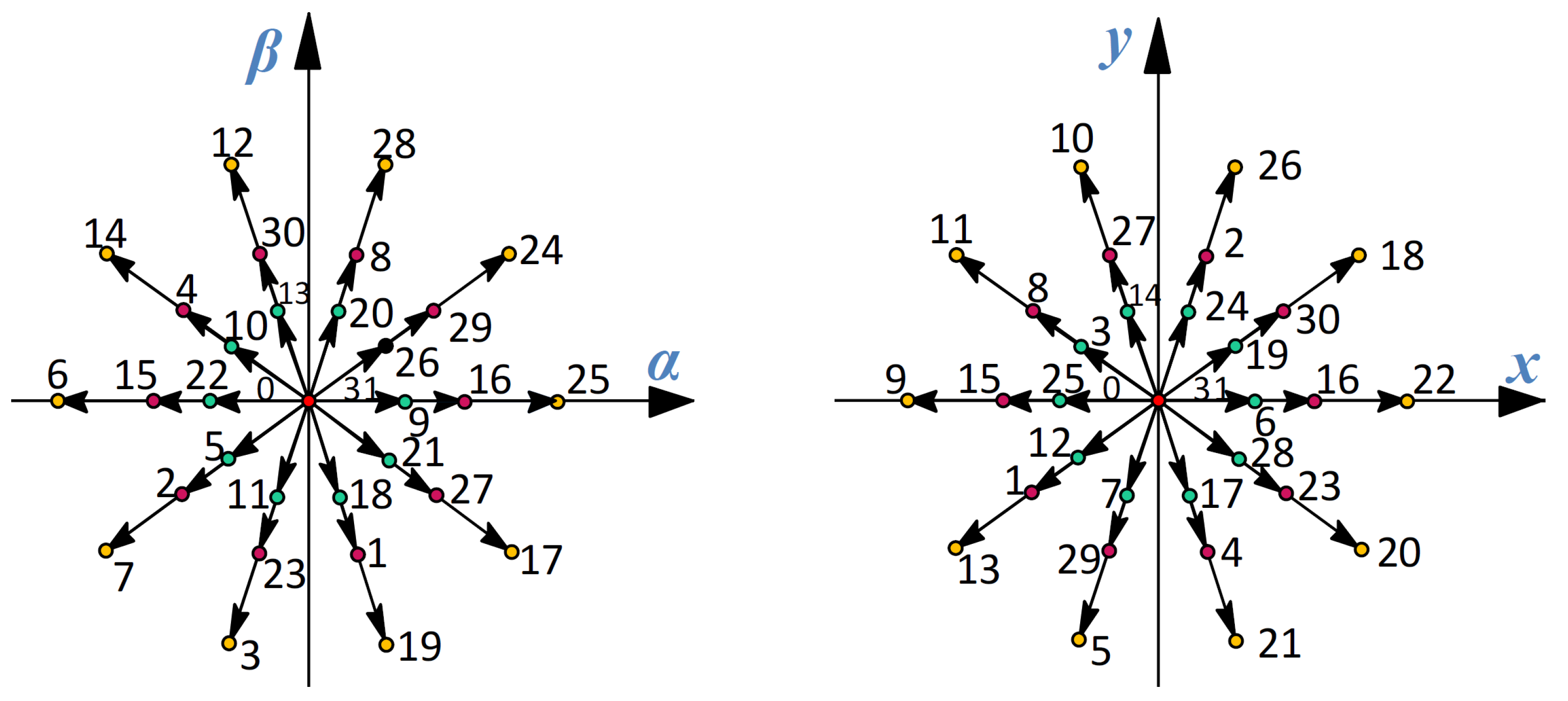
Figure 2.
Six-phase voltage constellation in and planes.

Figure 3.
Diagram of the experimental setup including photographs of various elements.

Figure 4.
Experimental results for (left) and for (right).

Figure 5.
Performance indices found for some combinations of controller parameters . The legend and horizontal rule apply to all graphs.
Figure 5.
Performance indices found for some combinations of controller parameters . The legend and horizontal rule apply to all graphs.

Figure 6.
3D distribution of pareto optimal values (top) and projections (botttom). Color indicates height (in the direction) and has been added to enhance perception.
Figure 6.
3D distribution of pareto optimal values (top) and projections (botttom). Color indicates height (in the direction) and has been added to enhance perception.

Figure 7.
Cubic surface (left) and its projection in the XY plane (right) including some horizontal cuts.
Figure 7.
Cubic surface (left) and its projection in the XY plane (right) including some horizontal cuts.

Figure 8.
Fitted surface (meshed lines) and some experimental data points forming lines A, B, C and D (see text for details).
Figure 8.
Fitted surface (meshed lines) and some experimental data points forming lines A, B, C and D (see text for details).

Figure 9.
Evolution of using the simplified MIT rule (top) and waveforms for a time period were the adaptated parameters are close to their final value 9 × 10 (bottom).
Figure 9.
Evolution of using the simplified MIT rule (top) and waveforms for a time period were the adaptated parameters are close to their final value 9 × 10 (bottom).


Table 1.
Electrical parameters for the experimental motor drive obtained by identification.
| Symbol | Parameter | Value |
|---|---|---|
| Stator resistance () | 1.63 | |
| Stator inductance (H) | 0.2792 | |
| Rotor resistance () | 1.08 | |
| Rotor inductance (H) | 0.2886 | |
| Mutual inductance (H) | 0.2602 | |
| Stator leakage inductance (H) | 0.0189 | |
| Nominal frequency (Hz) | 50 |
Publisher’s Note: MDPI stays neutral with regard to jurisdictional claims in published maps and institutional affiliations. |
© 2021 by the authors. Licensee MDPI, Basel, Switzerland. This article is an open access article distributed under the terms and conditions of the Creative Commons Attribution (CC BY) license (https://creativecommons.org/licenses/by/4.0/).
Share and Cite
MDPI and ACS Style
Arahal, M.R.; Satué, M.G.; Barrero, F.; Ortega, M.G. Adaptive Cost Function FCSMPC for 6-Phase IMs. Energies 2021, 14, 5222. https://0-doi-org.brum.beds.ac.uk/10.3390/en14175222
AMA Style
Arahal MR, Satué MG, Barrero F, Ortega MG. Adaptive Cost Function FCSMPC for 6-Phase IMs. Energies. 2021; 14(17):5222. https://0-doi-org.brum.beds.ac.uk/10.3390/en14175222
Chicago/Turabian StyleArahal, Manuel R., Manuel G. Satué, Federico Barrero, and Manuel G. Ortega. 2021. "Adaptive Cost Function FCSMPC for 6-Phase IMs" Energies 14, no. 17: 5222. https://0-doi-org.brum.beds.ac.uk/10.3390/en14175222
Note that from the first issue of 2016, this journal uses article numbers instead of page numbers. See further details here.