
Flexibility Estimation of Residential Heat Pumps under Heat Demand Uncertainty


Energy Economy and Application Technology, TUM Department of Electrical and Computer Engineering, Technical University of Munich, 80333 Munich, Germany
*
Author to whom correspondence should be addressed.
Energies 2021, 14(18), 5709; https://0-doi-org.brum.beds.ac.uk/10.3390/en14185709
Submission received: 5 August 2021
/
Revised: 25 August 2021
/
Accepted: 6 September 2021
/
Published: 10 September 2021
(This article belongs to the Special Issue Power Markets and Energy Demand)
Abstract
:With the increasing penetration of intermittent renewable energy generation, there is a growing demand to use the inherent flexibility within buildings to absorb renewable related disruptions. Heat pumps play a particularly important role, as they account for a high share of electricity consumption in residential units. The most common way of quantifying the flexibility is by considering the response of the building or the household appliances to external penalty signals. However, this approach neither accounts for the use cases of flexibility trading nor considers its impact on the prosumer comfort, when the heat pump should cover the stochastic domestic hot water (DHW) consumption. Therefore, in this paper, a new approach to quantifying the flexibility potential of residential heat pumps is proposed. This methodology enables the prosumers themselves to generate and submit the operating plan of the heat pump to the system operator and trade the alternative operating plans of the heat pump on the flexibility market. In addition, the impact of the flexibility provision on the prosumer comfort is investigated by calculating the warm water temperature drops in the thermal energy storage given heat demand forecast errors. The results show that the approach with constant capacity reservation in the thermal energy storage provides the best solution, with an average of 2.5 min unsatisfactory time per day and a maximum temperature drop of 2.3 °C.
1. Introduction
With the penetration of intermittent and fluctuating renewable energy generation positioned to increase in the coming years, there is a growing need for low-cost and practical Ancillary Services (AS) to absorb the renewable related imbalance between generation and demand [1]. Demand Response (DR), the ability to control electrical energy consumption based on power grid incentives, is emerging as a low-cost alternative to conventional fast-ramping generation resources [2]. Additionally, the study in [3] foresees that a complete electrification of the heating sector will eventually lead the heat pumps’ demand to reach 26% of the total electricity consumption in Europe. This places the heat pump dominant in the field of DR. Furthermore, the study in [4] has proved that energy savings of up to 80% can be achieved with the implementation of an optimal control of the HVAC with heat pumps. Therefore, special attention has been given to exploiting the applications associated with heat pumps.
In the literature, several works deal with the assessment of the flexibility given by building energy management systems. In [5], flexibility potential could be quantified by generating deviation from the optimal plan by adjusting the objective function with regard to energy consumption (low or high) solely in the timespan of flexibility. Meanwhile, it used a cost curve to present the additional associated costs. Similarly, another study performed simulations with a diversified thermostat set point of buildings to develop a novel demand response estimation framework [2]. In addition, the authors have performed a multi-agent-based simulation of three building cluster types and studied the impact of the available flexibility on the residual substation load. Although a high penetration of heat pumps and photovoltaic systems can violate the transformer’s limits, a significant improvement in the substation load can still be seen with the help of the Demand Side Management [6]. Moreover, it has been found that the flexibility of a building energy system is difficult to quantify using a single flexibility indicator. Therefore, the authors have proposed that flexibility needs to be evaluated in three dimensions: time, power and energy [7]. In addition, the key factors affecting the flexibility potential have been investigated over the last three years. In general, the flexibility available is affected by penalty signals, ambient temperature and the operations of the energy storage [8,9,10].
In particular, a number of studies have developed models to estimate the flexibility potential of the heat pump. The authors in [11,12] have provided an overview of the possible Demand Side Management applications in the field of heat pumps and evaluated its efficiency in providing peak shaving and thermal comfort. In [13,14], a generic flexible offer generation and evaluation process that extracts flexibility from heat pumps and other household devices is presented and incorporated in a unified model. As indicated in [1,15], an optimal control is imperative to obtain the maximum flexibility provided by a building’s energy system. An approach has been proposed that allows for the various available building datasets to be relied on to build the models required for optimization tools or dynamic simulations [15]. In addition, an approach to estimate the time-dependent flexibility potential of a heat pump system is proposed. It used a modified Optimal Power Flow (OPF) to evaluate the feasibility of the flexibility provision [16]. Furthermore, case studies have been performed to investigate the impact of the aggregation of heat pumps and uncertainties inherent in forecasts and building parameters [17,18]. It is revealed that it is beneficial to include domestic hot water (DHW) demand within the optimization model to deal with the high unpredictability of the DHW consumption. However, uncertainty in building parameters does not have a significant impact on the optimization of heat pump operation. In contrast, Thermal Energy Storage (TES) is essential to offer flexibility in the heat pump system, as indicated in [1,5,16]. Through active management and suitable scheduling schemes of the HP and the TES, it is possible to provide flexibility for the power system through sustainable energy buildings where the electricity supply is highly volatile [19].
For the provision of flexibility, the aforementioned research has mainly focused on the centralized coordination of controllable household devices. Meanwhile, the German government has used various support measures to continuously adapt flexibility provision to market developments [20]. A flexibility market is a concept for the utilization of flexibility, their efficient use and the assurance of a coordinated call-off [21,22]. Instead of passive participation, energy consumers have higher flexibility to enable a market supply that meets market conditions. In addition, the flexibility market allows for a “cellular” approach, where the flexibility requirements are determined on the scale of individual units, rather than a top-down approach based on an aggregate calculation of expected demand and supply [20]. Moreover, local flexibility markets enable an economically efficient solution to trade flexibility among distribution system operators and other participants (e.g., aggregators). This will incentivize the flexibility provision [23,24].
Although many studies have proposed methods to quantify flexibility, they tend to look at the response of the building or household appliances to external control signals from the top down. This means these approaches estimate flexibility only from a macroscopic perspective [1,13,17]. In addition, uniform prices and contracts for all flexibility provider will hurt their motivation to actively participate in the flexibility provision [25]. However, few studies have focused on the development of a tool to quantify the tradable flexibility to address future needs regarding flexibility markets and considered the benefits of using flexibility for prosumers. Moreover, user comfort may be affected by providing flexibility due to the unpredictability of DHW consumption [9]. However, this has not been discussed very much to date.
This paper aims to find a simple yet effective method to quantify the flexibility of domestic heat pumps without affecting the user comfort, while covering the gaps mentioned in the previous paragraph. Unlike the demand response approaches that consider mainly the reaction of residential units to external signals, the methodology in this paper quantifies the flexibility of residential heat pumps based on the optimized operating plan and the state of the TES and describes the flexibility in form of flexibility power and energy for each time block. This nature enables the day-ahead trading on the flexibility market. Furthermore, the capacity reservation in thermal energy storage is implemented to avoid the negative impact of flexibility utilization on the prosumer comfort. It is expected that the warm water temperature in the TES can be maintained above the set point at all times. To validate this concept, a forecast-simulation methodology has been used to test its effectiveness in dealing with the unpredictability of DHW consumption.
This paper is structured as follows. Section 2 provides the mathematical models applied to represent the heating and electrical system as well as the optimization algorithm. Section 3 introduces the methodology used to estimate the flexibility potential of heat pumps in three steps. Furthermore, a number of solutions to deal with the DHW consumption’s randomness is discussed in Section 4. Section 5 presents and discusses the obtained results, while Section 6 discuss the main findings and conclude the paper, respectively.
2. Modeling and Optimization
In this section, the modeling approaches of the heating system and the optimization algorithm using Mixed Integer Linear Programming (MILP) are introduced. All modeling and calculations processes are carried out in the framework of open-source software OpenTUMFlex. For more information, please refer to Supplementary Materials [26].
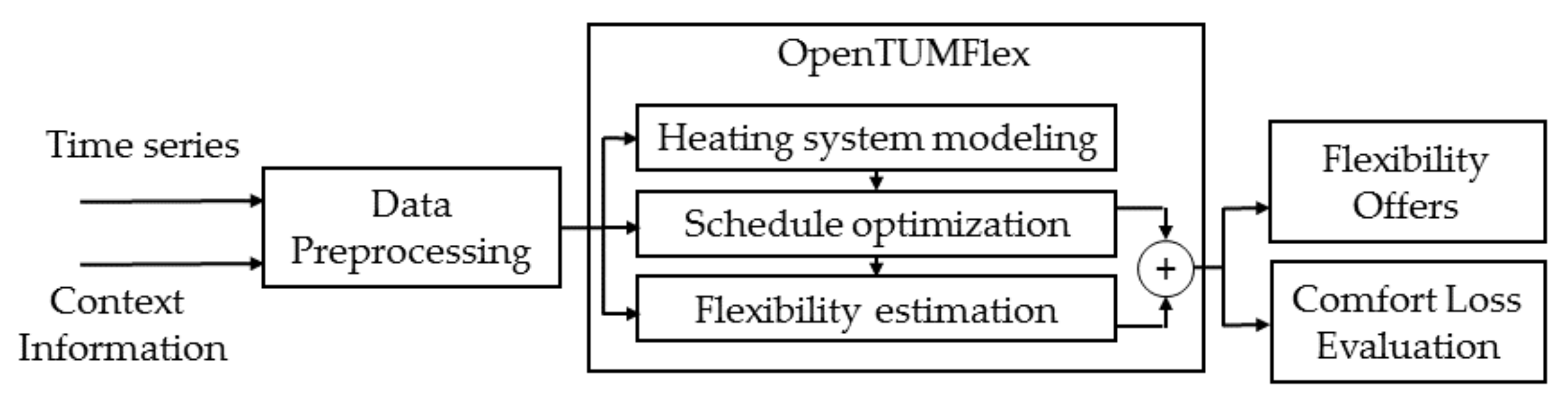
Figure 1 shows the general steps involved in flexibility generation. The flexibility estimation process begins with the gathering of the heat demand time series and available context information such as the technical parameters of the heat pump, electricity prices, etc. The next step includes the preprocessing of the raw information into an adequate format for analysis. The main steps include modeling the heating system required for the generation of the optimal operating plans. Subsequently, the solver integrated in OpenTUMFlex performs process scheduling and finds an optimal operating plan for the heat pump. Finally, the flexibility estimation step includes the derivation of new operating plan for the heat pump and the calculation of flexibility power and energy with regard to necessary technical restrictions. The last two steps visualize the flexibility power and energy in a graphical and table form and statistically evaluate the impact of unpredictable DHW consumption on prosumer comfort.
2.1. Models
The model used to represent the heating system consist of two main components: the HP, which generates heat, fulfilling the demands, and the TES, which serves as a buffer to avoid the simultaneity of generation and consumption.
2.1.1. Heat Pump
The heat pump is a component that uses electricity to generate heat. The ratio between the generated heat and electrical power is the Coefficient of Performance (COP). Mathematically, it can be described as follows:
Here, and represent the heat flow and electrical power. The higher the COP, the more efficient the heat pump. In this paper, ground-source heat pumps (GSHP) are considered. Their COP can be influenced by many factors. For GSHP, the COP is mainly affected by ground temperature and the supply temperature of warm water. To ensure the linearity of the model, the ground temperature and the supply temperature of the HP are set as parameters for each simulation. Based on the experimental data of the heat pump (Stiebel Eltron), the COP curve can be derived using the following formula:
where and are the supply and ground temperature, respectively. is the thermal power of the heat pump depending on the ambient temperature, given an average supply temperature of 60 °C. With regard to the operational behavior of the heat pump, it is assumed the HP has two working states without any modulation: on/off. Thus, a binary variable is used to describe the state of the heat pump operation:
In this equation, is the binary variable indicating the operational state of heat pump at a certain time step. The electrical power consumed can then be calculated by Equation (6).
There are also constraints avoiding the frequent switch on/off, which keeps the HP off for time steps once it is turned off and the heat pump on for time steps once it is turned on, as indicated in Equations (7) and (8). In this article, and are both set to 4, which means 1-hour minimum duration for switch on/off given each time step of 15 min.
2.1.2. Thermal Energy Storage
To provide flexibility and fulfill DHW and Space Heating (SH) demand, a heat storage with a spiral-tube heat exchange will be used. The combined storage consists of an internal heat exchanger to separate fresh water and heating water.
where is the energy stored in the TES, while and are the heat load of SH and DHW, respectively. Meanwhile, the State of Charge (SOC) is the level of charge relative to its capacity. The warm water temperature in the TES can be estimated by Equation (11), given that the TES is perfectly mixed.
2.2. Heating System
2.2.1. Heat Load
The heat load consists of SH and DHW. The heat load profiles for SH are derived based on the Hotmaps Project database, which is part of the Horizon 2020 Projects. The datasets have a temporal resolution of 1 h [27]. The year-specific profiles, generated based on the synthetic hourly profiles for typical days, are used for further simulation.
Regarding the region of NUTS2, DE21 (Upper Bavaria) was selected as the region where the case study was conducted. The specific heat demand refers to standard WSVO 95, which indicates a value of 100 /( · a). The heating area is assumed to be 140 m.
As the yearly heat demand profiles only offer a temporal resolution of 1 h and the normal time-step of flexibility estimation in OpenTUMFlex is 15 min, the heat demand of 1 h will be distributed linearly.
The software, DHWcalc, can provide the DHW consumption data. This model uses four categories of DHW to describe different DHW use patterns [28]. Each category has a specific occurrence probability and flow rate probability distribution. The assumptions applied in [28] have been used in this study as well and are shown in Table 1:
Where average flow rate is the expectation of the distribution and sigma is the standard deviation. Duration and portion are the assumed flow duration and share of flow amount for each flow type, respectively.
2.2.2. Assumption for Heating System
Considering the conclusion of [5], the thermal characteristics of the building are neglected and the static heat load from Section 2.2.1 is implemented to represent the SH load of the household. Therefore, a constant room temperature is assumed inside the house. This implies that the thermal inertia of the building is not taken into account to offer flexibility. These assumptions avoid exhausting the flexibility potential with regard to the thermal inertia of the building and can be treated as a buffering mechanism for possible comfort losses.
The supply temperature out of the heat pump was assumed as 60 °C, which avoids sanitary problems n DHW and increases the maximum heat capacity of the TES. A conventional heat pump cannot reach a supply temperature of 60 °C without a severe efficiency drop. Thus, for a higher supply temperature, a medium-temperature heat pump was considered. The reference and maximum temperature of the TES was set as 40 °C and 60 °C, which indicates that the SOC of the thermal energy storage is 0% and 100%, when the warm water inside is uniformly 40 °C and 60 °C, respectively. The TES was assumed to be perfectly mixed to make it possible to quantify the comfort loss without an enormous calculation burden.
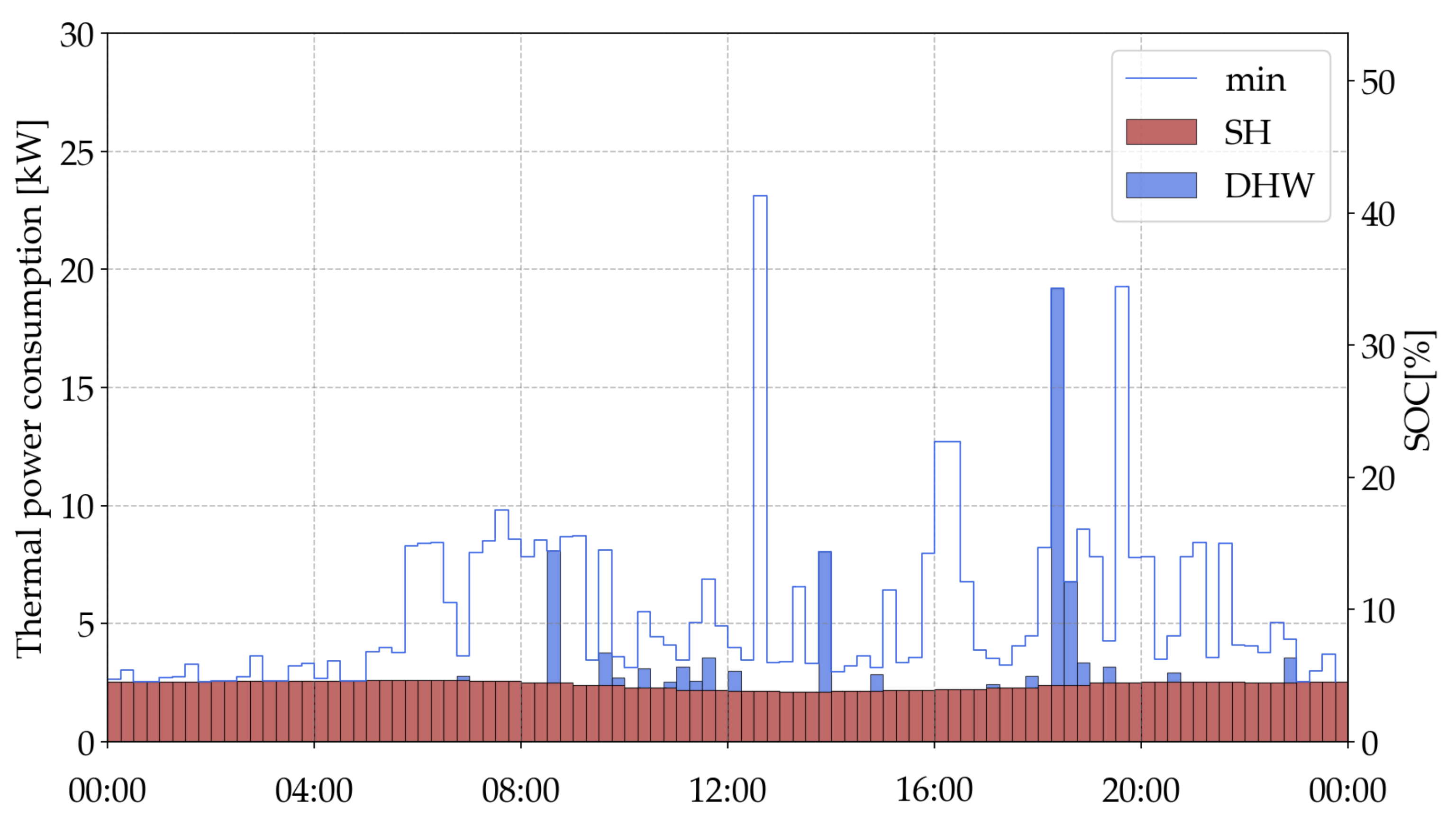
As the time resolution of the software DHWcalc was set up at 1 min to describe each type of draw-off, it does not fit the 15-min time interval in OpenTUMFlex. Therefore, the DHW heat demand calculated from DHWcalc will be averaged into a 15 min time interval to suit the formats in OpenTUMFlex. Regarding the DHW consumption forecasts, a naive forecasting method was implemented by averaging the last 30-days’ historic data. Subsequently, the thermal energy consumption within each time step can be obtained by integrating the required heating power. Based on the TES capacity, the required minimum SOC can be obtained for each time step. The minimum SOC considers both the trivial SH heat load and the possible extremely high DHW consumption that has occurred in the last 30 days. Therefore, the TES, with this minimum SOC, is capable of fulfilling the SH and DHW heat load simultaneously, even when forecast errors of DHW consumption occur. Repeating this process for all time steps, the minimum SOC curve for the TES with 600 L volume and 20 °C temperature spread can be estimated as the “min”, as shown in Figure 2. In addition, the heat loads of SH and DHW are shown as well.
2.3. Optimization
This section presents an optimization algorithm to coordinate the operations of all main household appliances. The objective of the optimization is to find a cost-optimal schedule of each appliance while fulfilling all the constraints. In general, theses components are considered in the HEMS: Electric Vehicle (EV), Photovoltaic (PV), Battery (BAT) and Heat Pump (HP). The other electrical and heat loads are treated as inflexible loads.
With regard to electricity balance, the sum of electrical generation and consumption must be equal. The relationship can be represented by Equation (13)
where power generation of each type is placed on the left side and power consumption on the right side. , and are the electrical powers consumed by PV, HP and EV, respectively. and indicate the power import and export with the grid. and represent the charging and discharging power of the battery. Charging and discharging cannot occur at the same time. is the inflexible load of the household. Similar to the electricity balance, the heat balance is constructed in the same way, such that the thermal generation and consumption must be equal:
On the left side of this Equation (14) is the thermal power of each heat generating device, including the discharging power of the TES, while the heat load and the charging power of the TES is positioned on the right side.
For the TES, the optimal end SOC should be determined by extending the original simulation time horizon. For instance, a 1.5-day simulation will be carried out first and the SOC of the time point at 24 h will be used as the optimal end SOC for the next 1-day simulation. To decrease the required computation time, the end SOC must be greater than the optimal end SOC [29].
According to the constraints and the models, the solver can minimize the total energy cost by scheduling the operation plan of each household appliance. The costs mainly cover the fuel and electricity cost, which is dependent on the gas and electricity prices. Thus, the objective function for this model can be formulated by Equation (15):
where and are the predicted gas price and electricity price, respectively. Based on the objective function, the solver will determine the optimal operation time of each household appliance.
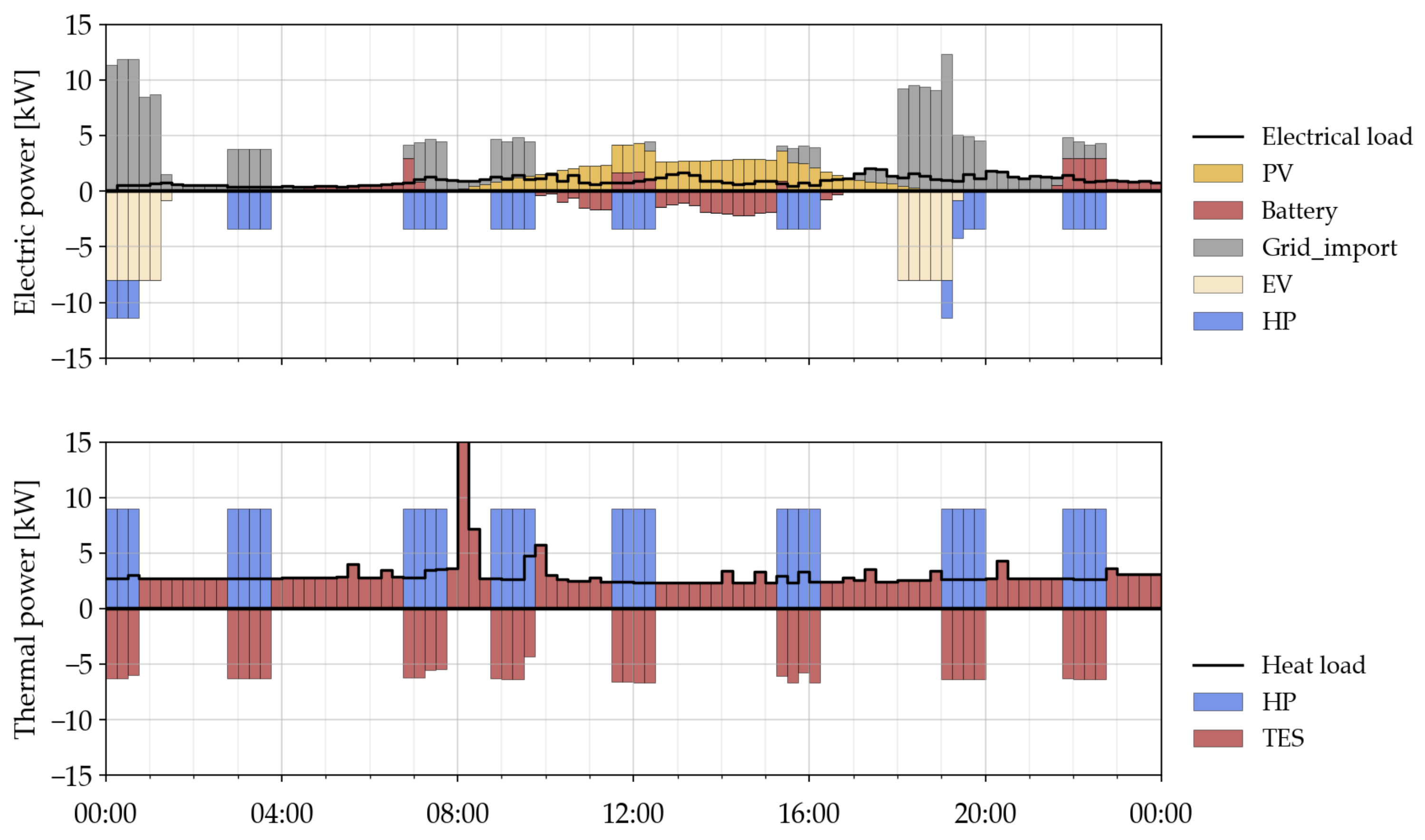
Since the objective function is linear and integer variables are utilized to represent the operational states of the HP, this optimization problem can be categorized as Mixed Integer Linear Programming (MILP), which can be easily solved by matured solvers (Cplex, GLPK or Gurobi) within several minutes when the optimization is within 24 time steps. Figure 3 shows an example of the optimization results.
3. Flexibility Estimation
In this section, specific methods to estimate flexibility are introduced. Flexibility of the heat pump can be regarded as the possibility of shifting the HP operation during the day. Based on the optimal operation plan of the HP, potential deviations can be offered at each time step. They are distinguished into two types. Positive flexibility means turning off the HP in situations where it would otherwise run, while positive flexibility indicates that the heat pump is forced on when it would usually be turned off. The flexibility provision is not arbitrary and requires many restrictions. They are usually divided into three types:
- Switch point;
- Remaining capacity of thermal storage system;
- Available regeneration time.
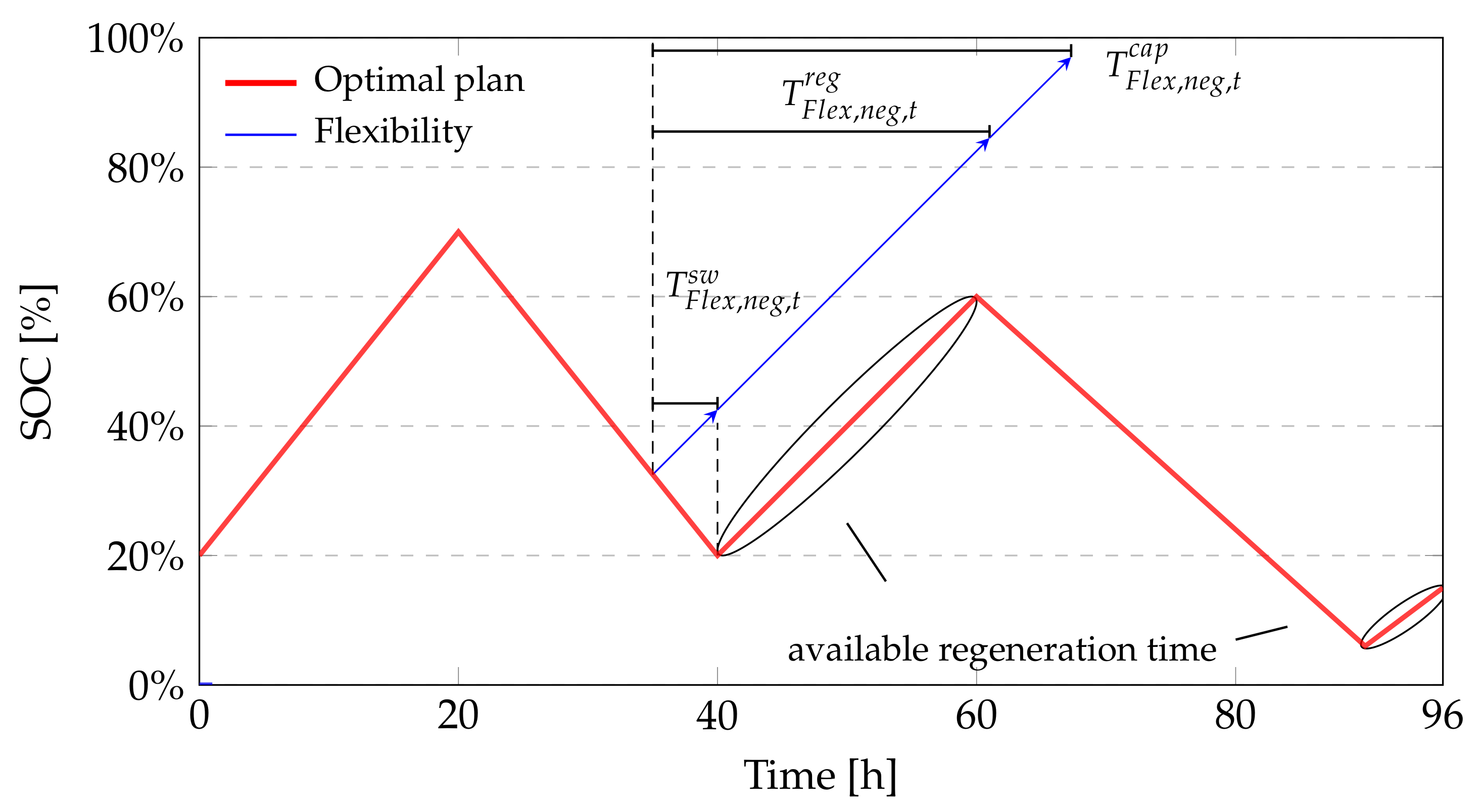
The first restriction implies that the flexibility can only be offered until the next switch point. As Figure 4 illustrates, positive flexibility can only be provided when the heat pump is on, as it cannot reduce the electrical load by changing the operation of the heat pump when it is already off. Thus, positive flexibility can hold up until the next switch point. In contrast, negative flexibility is available when the HP is off. Therefore, the duration limit of flexibility regarding the first restriction can be formulated by Equation (16):
Here, is the time step number until the next switch point, while t is the time step by which the flexibility potential is estimated.
Figure 4.
Restrictions with regard to flexibility estimation: switch time, capacity and regeneration time.
Figure 4.
Restrictions with regard to flexibility estimation: switch time, capacity and regeneration time.

Another restriction is the remaining capacity of the TES, because the heat pump cannot keep charging or discharging when the thermal storage is full or empty. With regard to positive or negative flexibility, the duration limit can be obtained by Equations (17) and (18), respectively:
where and is the average thermal power of the heat pump and heat load within next two hours, which is the typical duration of HP flexibility. With respect to positive flexibility, the duration limit indicates how many time steps the TES can afford without the heat supply from the heat pump. Negative flexibility, however, requires a low SOC of the TES. The higher the SOC, the smaller the remaining space for excessive heat generated from the HP. Therefore, the remaining capacity of the TES is used to calculate the flexibility duration limit of negative flexibility.
After delivering the flexibility, the system states will change and the original schedule for the time becomes infeasible. Hence, the operation plans for each devices need reoptimization during the interval from the flexibility duration termination to the end of one day. The reoptimization aims to realize the same system states at the end of the day as the original plan, such as the SOCs of TES. Therefore, it is imperative to generate enough time steps for the regeneration of TES. Following the positive flexibility provision, the thermal energy stored in TES decreases and more charging time is needed afterwards for the heat pump to produce heat, so that it can nearly reach optimal SOC in the end. The same is true for negative flexibility: if the remaining available regeneration time is insufficient to consume the additional thermal energy that is generated, the SOC of the TES will exceed the required amount by too much. As a consequence, the duration of flexibility with respect to the available regeneration time is restricted by Equations (19) and (20), in the timestep number.
where and are the last timestep of the delivered flexibility and the whole timespan. Here, the Iverson Brackets, which take the value 1, for which the statement is true, are used to count the the number of suitable timesteps.
As all the three types of restrictions for the flexibility duration are already known, the final flexibility durations have to satisfy all of the above, so the minimum of these values is taken:
According to the flexibility duration, the flexibility power and energy, which are the average power and the total energy delivered within the flexibility, can be obtained by Equations (22) and (23):
The flexibility power indicates how much power deviation controlling of the heat pump can provide and the flexibility energy is the integral of the flexibility power within the flexibility duration. This flexibility estimation process will iterate for every timestep being considered, and acquire flexibility for the whole interval.
4. Methods Dealing with Stochastic Characteristic of Hot Water Consumption
4.1. Reservation of Minimum SOC
Since the day-ahead forecast of the heat load of SH is accurate enough, its forecast error can be neglected. However, the heat load of DHW is strongly affected by the user behavior and reflects an obviously stochastic characteristic, especially at the level of a single residential unit. Consequently, unexpected situations could occur while delivering the flexibility of heat pump, e.g., the temperature of warm water inside is not sufficient for trivial usage. To avoid these unwanted situations, the approach of capacity reservation is applied to cope with the unpredictability of DHW consumption. Using this approach, a certain percent of the heat capacity of TES must be reserved as a buffer, in case of unexpected user behavior and DHW consumption. The basic idea is to record the maximum warm water consumption in the last 30 days for each time step and recognize it as the possible worst case, which would also happen in the viewed day. This will ensure that the temperature of TES would not decrease below 40 °C. Nevertheless, the reservation of partial space in TES places additional constraints on the optimization of heat pump operation and flexibility estimation, which will increase energy costs for the heating system and reduce the available flexibility offered by the heat pump.
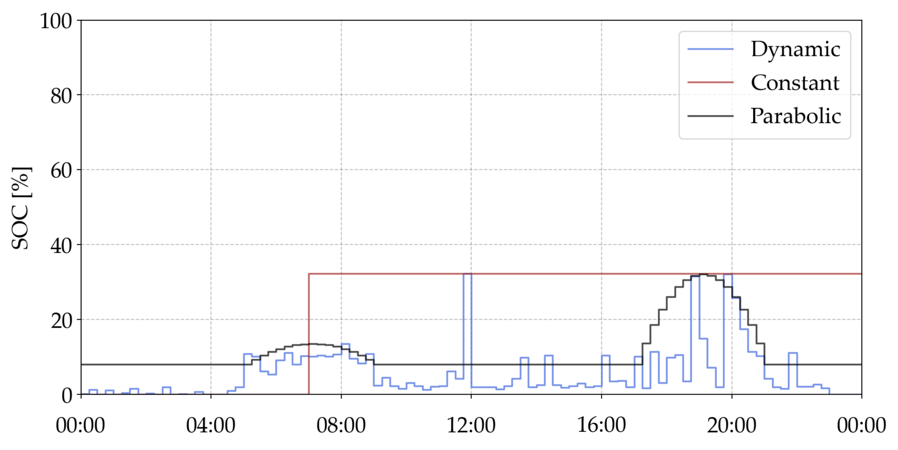
For the concept that the household has one TES for both SH and DHW, three options are considered to cover up the unpredictability of DHW consumption, in the form of the required minimum SOC curve in Figure 5:
- 1.
- Dynamic: use the maximum DHW consumption for each 15 min from the last 30 days to represent the potential risk of high consumption peaks;
- 2.
- Constant: use overall maximum DHW consumption from the last 30 days for the period 7:00–24:00;
- 3.
- Parabolic: use the parabolic curve to cover the typical peaks of one day.
Figure 5.
Minimum SOC curves: dynamic, constant and parabolic.

As seen from Figure 5, the first option generates a dynamic limitation curve, which changes itself every time step. The dynamic curve finds the maximum DHW consumption for each 15 min from the last 30 days and uses it to directly represent the potential DHW consumption peaks. This means that the possibility that the required thermal energy for DHW exceeds these thresholds is nearly 0%, even when forecast errors occur. Therefore, the influence of stochastic user behavior on the DHW consumption would be weakened. In comparison with the dynamic curve, the curve with constant values part of the time uses the overall maximum value of DHW-15min-consumption within the last 30 days to set a one-day minimum SOC value for TES from 07:00 to 24:00. The period from 00:00 to 07:00 is not taken into account because there is usually no heat consumption during this time period. This option ensures additional safety margins by raising the limits for most of the day. It also reduces the optimization complexity by simplifying the MILP problem. Another option with the parabolic limit finds a compromise between the first and second option. First, it gives a baseline for the whole day, which is a quarter of the maximum. Further, the peak hours in the morning and evening will be dealt with separated maximum values at these times, respectively. The amplitude and duration of the peak hours depends on peak flow rates and the assumed possibility distribution. Finally, a parabolic curve is used to reflect the importance of different times within the peak hours. Stricter restrictions are given at times when peak DHW consumption is more likely to occur. This solution will bridge the unexpected appearance of large DHW loads and keep user comfort unaffected.
4.2. Evaluation of Performance
Evaluation of the performances of different options require adequate evaluation methods. As the main purpose of this article is to provide flexibility service by heat pump without affecting the user comfort, the evaluation procedure concentrates on two factors: total flexibility energy and unsatisfactory time. To simply the assessment of flexibility potential, only the quantity of available flexibility is taken into account. For instance, the evaluation sums up all the offered flexibility energy for the whole day, but neglects the average flexibility duration. Additionally, the positive and negative flexibility will be treated equally. Therefore, the total flexibility energy is estimated with Equation (24):
With regard to the assessment of influences on user comfort, the unsatisfactory time and temperature drops are applied to perform the negative effects of unforeseen DHW consumption. Here, the reference temperature of TES (40 °C) is assumed to be the lowest temperature that can still meet the comfort requirements of the user. Once the temperature drops below 0 °C, its duration will be counted as unsatisfactory time. Meanwhile, the magnitude of the warm water temperature drops will be described by an additional parameter, temperature drop, with the assumption that every 5% SOC decrease below 0% corresponds to 1 °C temperature drop. For the whole day, the overall temperature drops are estimated by root–mean–square deviation (RMSD) while assuming the expected value as 0 °C. The RMSD describes how far the actual temperature deviates from the minimum required temperature and shows the severity of large temperature drops:
5. Results and Discussion
In this chapter, the results of a case study will be demonstrated. The basic settings and input data come from Section 2. The minimum run time and pause time of the HP is set at 2 h. The timespan of the simulation is 30 days (January). First, the general format of the flexibility estimation results is introduced. Then, the three different options handling the stochastic behavior of DHW consumption will be compared based on the aforementioned performance evaluation methods.
5.1. Flexibility Offers
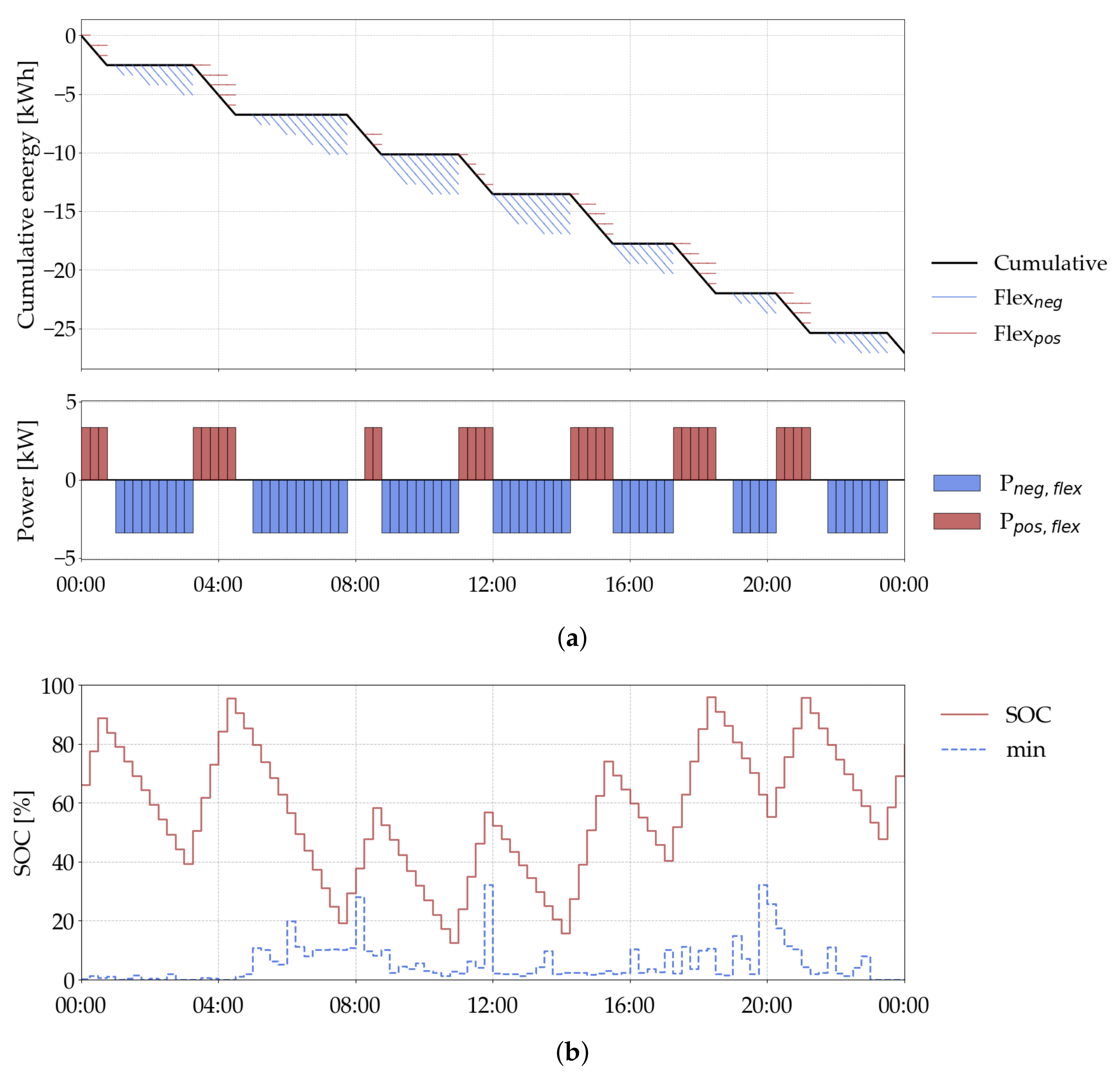
Following the estimation procedure introduced in Section 3, the flexibility potential of the heat pump can be quantified properly. A one-day example is demonstrated with Figure 6. Here, the total electricity consumption of heat pump is illustrated by the black line. The value is always negative because, in the context of OpenTUMFlex, all the energy consumed has negative values. Additionally, the blue and red lines, which are derived from the black line, are the flexibility of the heat pump, which can potentially be utilized by the system operator if needed. The horizontal width of the blue and red lines represents the flexibility duration and the vertical height means the flexibility energy for each time step. Comparing this diagram with the SOC curve below, their relationship is clearly visible. When the heat pump is turned on, the SOC of TES will increase, as well as the absolute value of cumulative energy. Afterwards, the flexibility of the heat pump will be estimated by Equations (16)–(18). The heat pump cannot always offer flexibility up until the next switch point because the TES becomes full or empty before the switch point if the flexibility lasts longer. For instance, in the time period between 11:00 and 12:00, all the flexibility offers are shorter than half an hour because of the DHW consumption peaks at 12:00. Therefore, the flexibility can only be partially utilized during this period. The flexibility power for each time step is shown in the lower diagram.
Flexibility offers can also be summarized in tabular format, which facilitates the trading process in the flexibility platform. A prosumer can use OpenTUMFlex to generate flexibility offers in tabular form and upload it directly to the trading platforms. Table 2 provides an example of how the tabular format of flexibility offers looks like within the period duration of 16:00–17:45. Here, the scheduled power consumption based on the optimal operational plan, its corresponding positive and negative flexibility power and energy can be clearly obtained.
5.2. Comparison of Methods Dealing with Unpredictability
As mentioned in Section 4.1, three different options handling the unpredictability of DHW consumption would avoid the negative effects of flexibility provision on user comfort. The basic idea of these options is to set a lower bound of SOC of TES to deal with the unexpected situation. To compare the performance of three different options, a 15-day case study was performed. The simulations were divided into two sessions for each option: forecast and validation. The optimal operation plan generated in the forecast session needed to be reviewed in a validation session. In the forecast session, the DHW consumption used its average value of the last 30 days, whereas the actual demand profile of DHW was utilized in the validation session. The calculation of flexibility potential and unsatisfactory time of the heat pump was performed for 30 days in a row, given weather data history from the last 30 days, gaining relatively convincing results. In the simulation round, the comfort loss was considered to occur when the SOC of TES fell below 0%, because the supply temperature for SH and DHW became lower than 40 °C. The unsatisfactory time and weighted average temperature deviation are summarized for each option.
- Forecast: generate optimal schedule for heat pump day-ahead based on predefined restrictions;
- Simulation: test if the generated optimal schedule of the heat pump can fulfill the minimum comfort requirement in the viewed day.
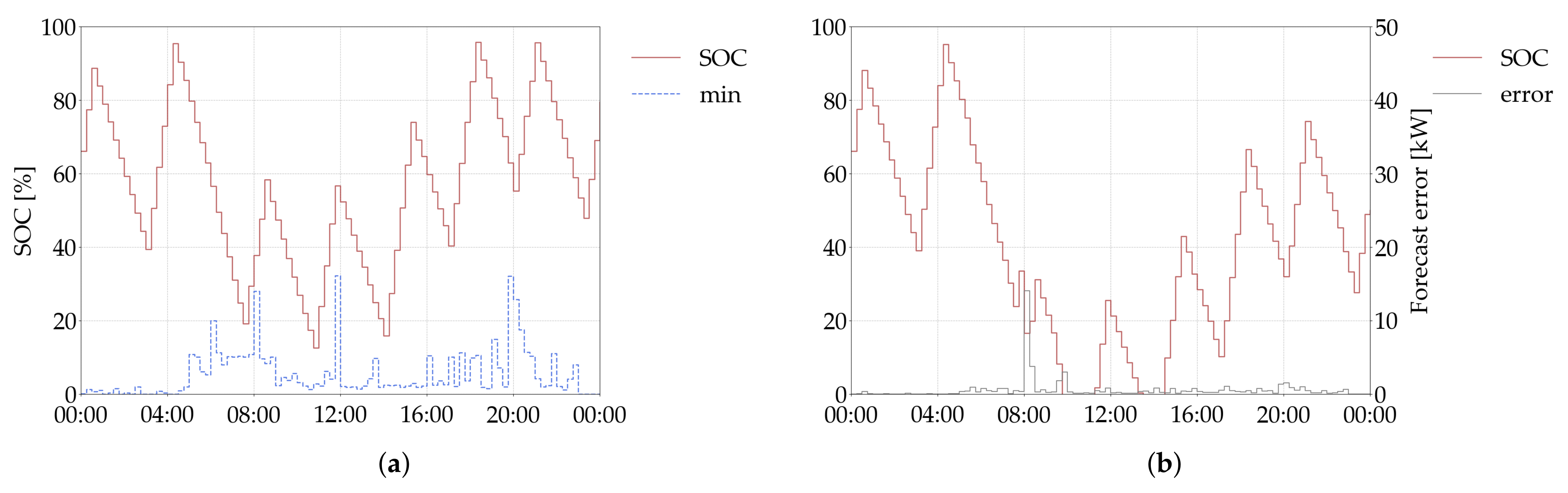
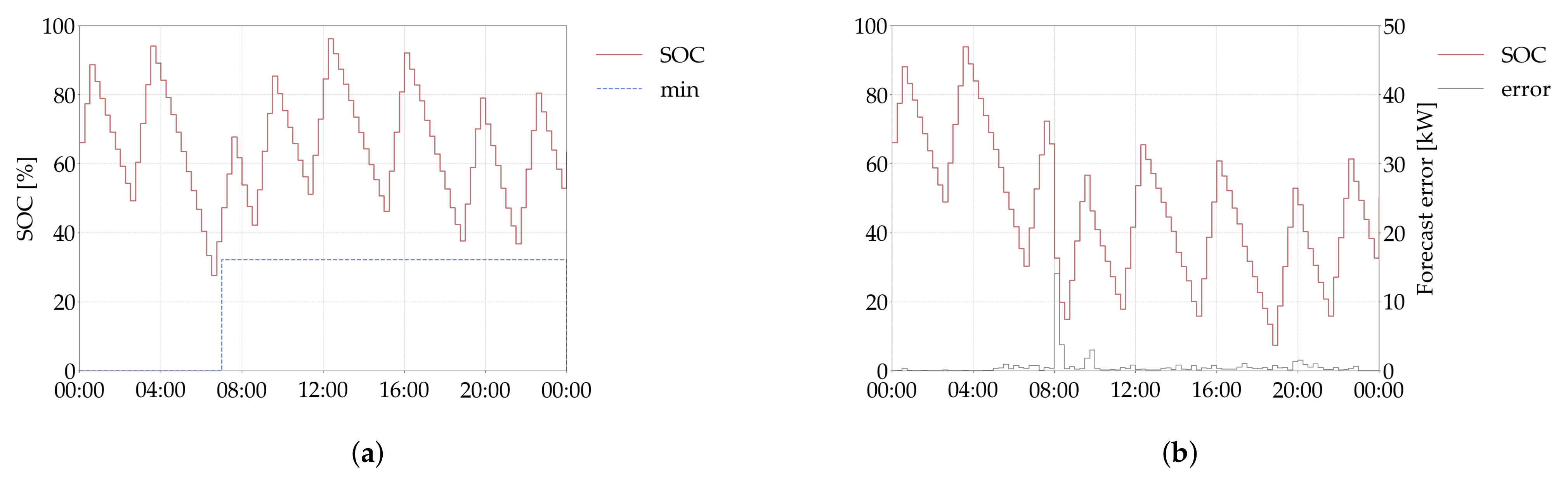
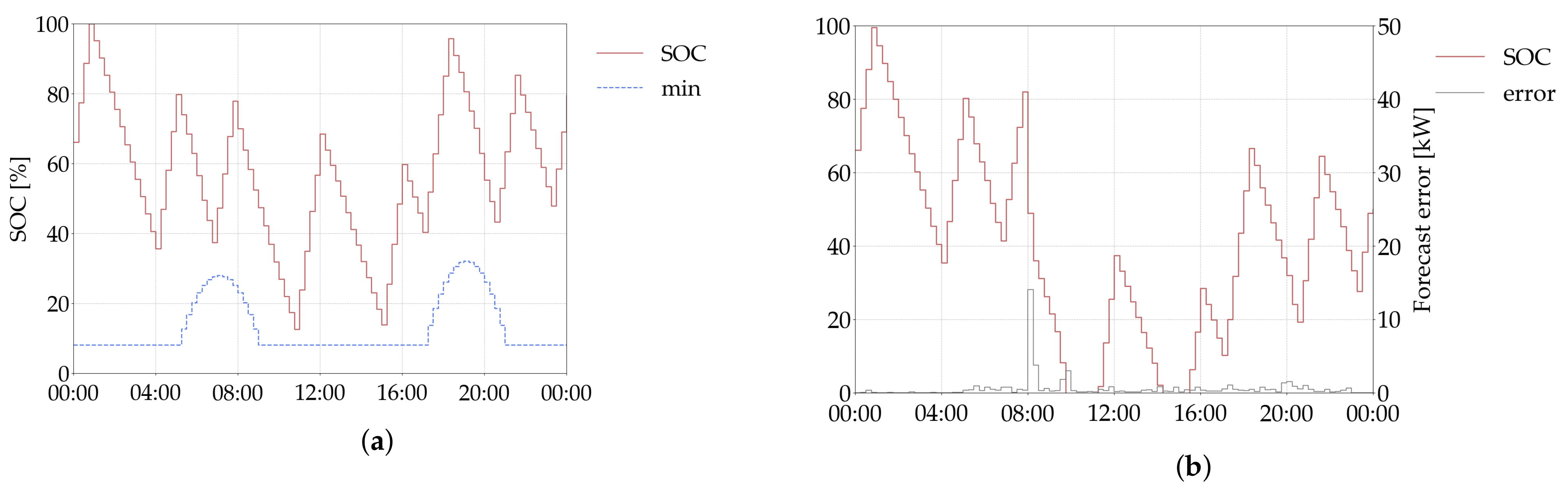
In Figure 7, Figure 8 and Figure 9 the results of the 1-day simualtion based on different options are illustrated as an example. In the forecast session (a), both the SOC profile and the lower bound of the TES SOC are demonstrated. In the simulation session (b), both the SOC profile and the unsigned forecast errors are represented. This makes it easy to compare the SOCs in these two sessions and observe when the forecast errors occur.
In Figure 7, the dynamic constraint used to cover the stochastic DHW usage is applied. The red line indicates the SOCs over the day. It can be seen the SOCs of the TES stay always in the required range, between the full state and the minimum bound determined by a predefined dynamic curve. By applying these extra limits for the SOC of the TES, it is expected that the reserved fraction of the thermal storage capacity can provide a “safety” margin for prosumer comfort, which means that the warm water temperature in the TES should not drop below a certain threshold even if there is a serious prediction error in the DHW consumption. To test its performance, the simulation session is needed. Given that the time schedule of the heat pump on the viewed day is unchanged, the real SOC curve of TES can be obtained by simulating the heating system again with actual DHW consumption instead of forecasts. Due to some unpredictable DHW consumption, as indicated by the grey lines in (b), it can be observed that the SOC of TES drops below 0% between 10:00 und 14:00. This means the comfort loss occurs because of the relatively low SOC states of TES in this period. This would appear once the DHW consumption on the observed day greatly exceeds the long-term average, because the forecast of the DHW consumption uses the average of the last 30 days. From (b), it is obvious that the largest forecast error occurs at 08:00. As a result, the SOC of the TES decreases by 30% after this time point, which further leads to a temperature drop of the warm water in the TES below 40 °C.
Similarly, this procedure can be performed for the case with a constant bound of SOC. The advantage of using a constant bound of SOC is that it provides a higher “safety” margin to cope with the unpredictable DHW consumption. However, it reserves more capacity in the TES and may cause losses in the flexibility potential, because the volume of the TES offering flexibility is not exhausted. In Figure 8, a better performance can be viewed when comparing (a) and (b), because the constant constraint avoids the low-SOC situation and allows for an additional buffer for the prosumer comfort. Here, the SOC of TES remain in the required range in the simulation session.
In addition, a combination of the first and second option would be meaningful as an alternative solution for capacity reservation in the TES, namely a parabolic lower bound. This option gives a moderate “safety” margin compared to the other options and is used to find a better balance between the user comfort and the flexibility potential. According to the simulation results, the scenario with parabolic limit shows no obvious improvement in Figure 9.
The analysis above refers to this 1-day simulation and only gives a brief overview of the impacts of different options. In the next section, the advantages and disadvantages of each option will be analyzed quantitatively in a statistical way with the help of the indicators discussed in Section 4.2.
5.3. Evaluation of Methods for Capacity Reservation
In order to quantitatively analyze the advantages and disadvantages of each option, the indicators discussed in Section 4.2 will be used, including total flexibility energy, unsatisfactory time and temperature deviation. Additionally, the situations after using flexibility will also be discussed. As when and how much flexibility would be required by the system operator is unknown, the unsatisfactory time and temperature deviation after using flexibility are only roughly estimated by assuming that each flexibility is equally likely to be utilized by the system operator. The acquired values can still demonstrate how flexibility usage will influence these indicators.
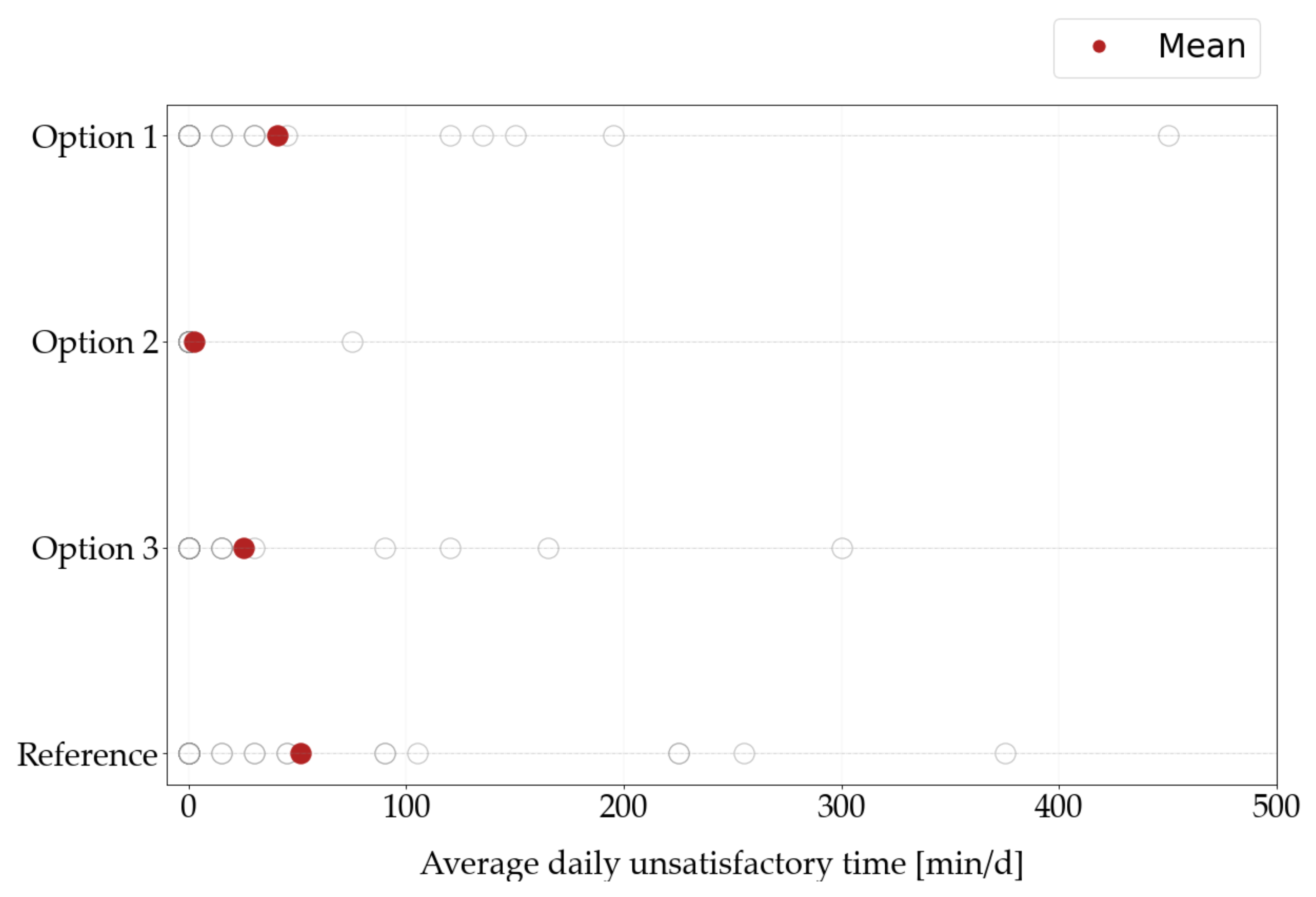
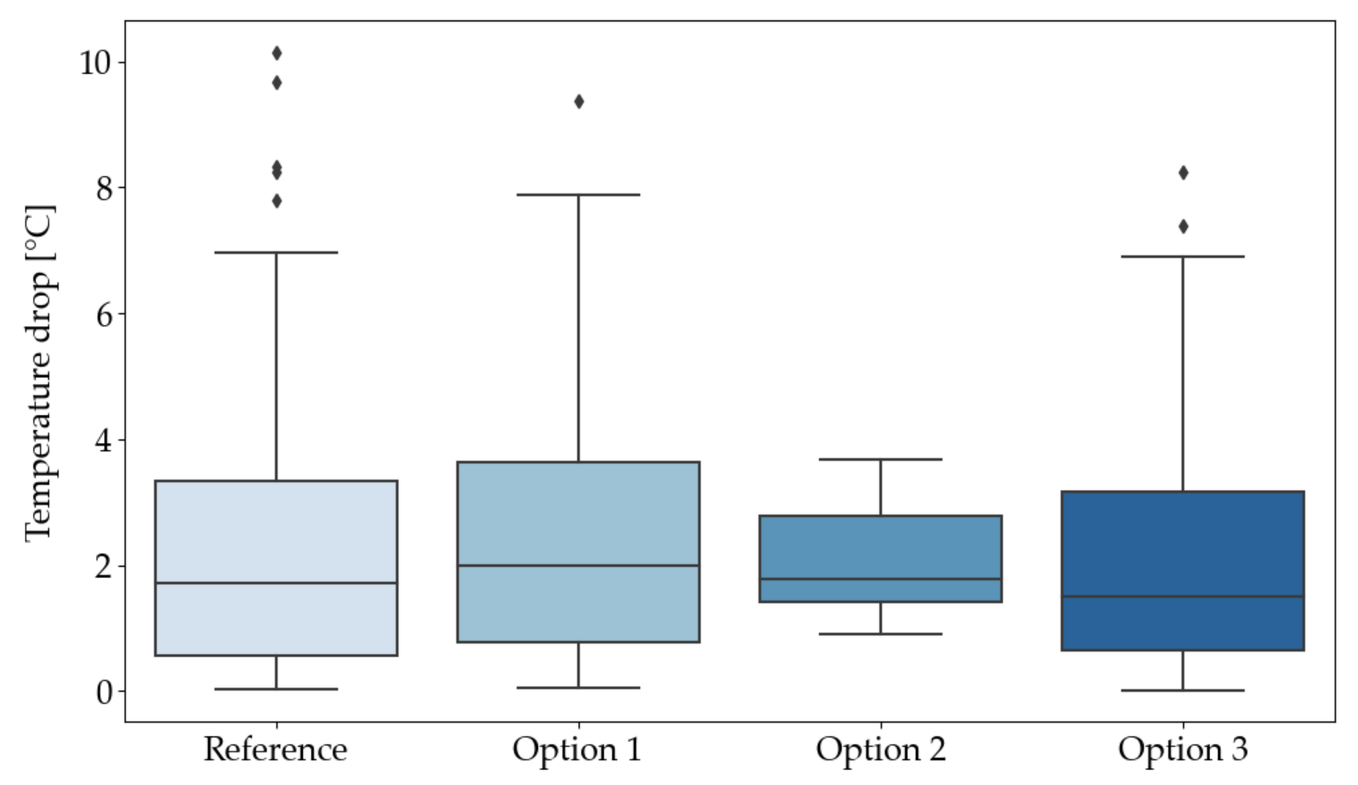
As shown in Figure 10, the unsatisfactory time denotes the negative impact of inaccurate DHW consumption forecasts on customer comfort. Within the simulation results of 30 days, option 2 with constant SOC restriction has the best performance, with a maximum unsatisfactory time of 75 min/day and mean value of 2.5 min/day, while others lead to more unsatisfactory times in terms of magnitude and quantity. In addition, the distribution of temperature drops in every 15 min time-block can be observed in Figure 11. They all have about the same average value. Nevertheless, option 2 with constant SOC restriction still has a small degree of variation, in which the most severe temperature drop is limited to 3.7 °C.
Table 3 summarizes the evaluating indicators. In general, all three options resulted in better performance compared to the reference scenario. Among the solutions, option 1 with dynamic restriction provides slightly more flexibility potential, while option 2 with constant restriction produces the least flexibility. Nevertheless, the differences in the available flexibility energy among the three options are not particularly noticeable. As opposed to this, the unsatisfactory time and temperature drop show a significant difference. The prosumer will notice little comfort loss in the scenario with a constant SOC lower limit, as its unsatisfactory time has a mean value of 2.5 min per day. In contrast, the results imply that the prosumer will suffer from comfort losses for 41.0 min for the first dynamic option, and 25.5 min for the parabolic one on a daily average. Simultaneously, these two options have reached 2.9 °C and 2.7 °C of temperature drop, statistically. The mean value here is slightly greater than these in Figure 10 because it also considers the outliers. Furthermore, how the flexibility usage will influence these evaluating indicators is revealed. In general, the influence of flexibility usage on the unsatisfactory time is not certain, although temperature drops become greater. In summary, either option, as it stands, is effective in reducing the impact of the stochasticity in DHW consumption. In the case of using option 2, there is only an average of around 2.5 min per day when the water supply temperature becomes too low, and the maximum temperature drop is within 2.3 °C. Therefore, the comfort of the prosumer is only affected to a fairly small extent, when he prepares to offer flexibility through this capacity reservation strategy.
To conclude the results from the case study, the three options suggest a slightly differentiated flexibility potential. Nevertheless, the simple strategy with a constant SOC lower bound for the TES performs best with regard to the unsatisfactory time and the temperature drop and should be proposed to deal with the demand uncertainty in future research.
5.4. Comparison of Flexibility Utilization Approaches
From the previous studies, there are lots of approaches studying the demand flexibility of heat pumps. In [8], the author uses a novel methodology, Flexibility Function, to characterize the energy flexibility. It mainly investigates the demand response curve of different types of buildings to penalty signals and uses indicators to quantify and evaluate the cost-saving potential of using this method. This study gives a good perspective to exploit the flexibility potential of buildings and districts with regard to diverse penalty signals (price, CO2, etc.). However, it only estimates the flexibility from a macroscopic perspective, leaving all control of the household appliances to the intelligent controller, without accounting for the prosumer comfort. In [10], it focuses on proposing new control strategies that maximize the gains from the demand side response. It uses complex modeling to make the results more convincing. At the same time, however, the complexity of its models makes its application elsewhere difficult. In addition, it does not consider the benefits of using flexibility for prosumers from an economic perspective. In [30], the time series of the flexible power consumption of the heat pump is optimized with regard to peak power reduction and load factor increase. Hence, its objective is to find an operating plan of the heat pump that is optimal for grid operation. This methodology can estimate the impact of demand responses of the heat pump on the grid, but requires a centralized control of a pool of heat pumps. In addition, this approach is not feasible to generate flexibility offers of individual residential units. Therefore, the research results cannot be implemented directly in the flexibility trading.
In contrast with these previous studies, this paper focuses on the decentralized management of the flexibility, instead of the centralized control or responses to penalty signals. The prosumers themselves decide the operating plan of the heat pump by Home Energy Management System and trade the alternative operation options of the heat pump on the flexibility market. Therefore, it describes an approach to utilize the flexibility from a microscopic perspective. Additionally, the methodology evaluate the demand flexibility by indicators such as flexibility power, energy and duration with a time interval of 15 min. This nature enables the trading on the flexibility market. Furthermore, this study investigates the warm water temperature drops inside the TES when offering flexibility and reserves a fraction of the thermal storage capacity in coping with the risk of comfort losses. The simulation results of 30 days denote that a constant SOC lower bound for the TES results in the best performance.
6. Conclusions
This paper proposes an novel approach to quantifying the flexibility of heat pumps combined with a thermal energy storage with regard to necessary technical restrictions. It suggests the decentralized flexibility management, which allows the prosumers to manage and utilize the residential flexibility actively. Furthermore, it analyzes the impact of offering flexibility on the thermal comfort of prosumers for the first time, and incorporates a viable solution to cope with the risk of unpredictable domestic hot water consumption. From the results, it is revealed that the capacity reservation in the thermal energy storage using a constant state of charge lower bound achieves the best performance. The simulations with this solution indicate that there is an average of 2.5 min unsatisfactory time per day and the maximum temperature drop never exceeds 2.3 °C given a predetermined operation schedule of the heat pump. Therefore, the proposed methodology enables the day-ahead flexibility trading on the local market to address future needs regarding flexibility markets and increases the prosumer acceptance, offering flexibility by reducing their discomfort, which contributes to energy transition in the long term.
All presented models algorithms are incorporated as an open-source tool in OpenTUMFlex for the interested parties and provide them with the opportunity to integrate the implemented methods for their research such as the investigation of the flexibility potential in Home Energy Management System and the local flexibility market design. Within the framework of OpenTUMFlex, the proposed flexibility quantification methodology will be further developed and evaluated. Specifically, more data will be collected to cover more types, such as air-source heat pumps from different manufacturers. The possibility of applying non-linear optimization programming will have to be investigated to find a better balance between model accuracy and computation time. Additionally, the development of aggregation methods will contribute to the widespread use of the flexibility potential in domestic heat pumps.
Supplementary Materials
The model OpenTUMFlex is open-source and accessible online at https://zenodo.org/record/4251512.
Author Contributions
Conceptualization, M.Z. and Z.Y.; methodology, Z.Y.; software, M.Z., Z.Y. and B.K.N.; validation, Z.Y.; formal analysis, Z.Y.; writing, Z.Y.; supervision, P.T.; project administration, P.T.; funding acquisition, P.T. All authors have read and agreed to the published version of the manuscript.
Funding
The German Federal Ministry for Economic Affairs and Energy, Bundesministerium für Wirtschaft und Energie, funded this research under the grant number 03SIN109.
Data Availability Statement
Publicly available datasets for heat load profiles were used in this study. This data can be found here: https://wiki.hotmaps.hevs.ch/Home.
Conflicts of Interest
The authors declare no conflict of interest. The founding sponsors had no role in the design of the study; in the collection, analyses or interpretation of data; in the writing of the manuscript nor in the decision to publish the results.
Abbreviations
| AS | Ancillary Service |
| ASHP | Air Source Heat Pump |
| BAT | Battery |
| CHP | Combined Heat and Power |
| COP | Coefficient of Performance |
| DHW | Domestic Hot Water |
| DR | Demand Response |
| EV | Electric Vehicle |
| HEMS | Home Energy Management System |
| PV | Photovoltaic |
| SH | Space Heating |
| TES | Thermal Energy Storage |
References
- Finck, C.; Li, R.; Kramer, R.; Zeiler, W. Quantifying demand flexibility of power-to-heat and thermal energy storage in the control of building heating systems. Appl. Energy 2018, 209, 409–425. [Google Scholar] [CrossRef]
- Yin, R.; Kara, E.C.; Li, Y.; DeForest, N.; Wang, K.; Yong, T.; Stadler, M. Quantifying flexibility of commercial and residential loads for demand response using setpoint changes. Appl. Energy 2016, 177, 149–164. [Google Scholar] [CrossRef] [Green Version]
- European Commission. Joint Research Centre. Decarbonising the EU Heating Sector: Integration of the Power and Heating Sector; Publications Office of the European Union: Luxembourg, 2019. [Google Scholar] [CrossRef]
- Franco, A.; Miserocchi, L.; Testi, D. Energy Intensity Reduction in Large-Scale Non-Residential Buildings by Dynamic Control of HVAC with Heat Pumps. Energies 2021, 14, 3878. [Google Scholar] [CrossRef]
- De Coninck, R.; Helsen, L. Quantification of flexibility in buildings by cost curves—Methodology and application. Appl. Energy 2016, 162, 653–665. [Google Scholar] [CrossRef]
- Langer, L. An Optimal Peer-to-Peer Market Considering Modulating Heat Pumps and Photovoltaic Systems under the German Levy Regime. Energies 2020, 13, 5348. [Google Scholar] [CrossRef]
- Stinner, S.; Huchtemann, K.; Müller, D. Quantifying the operational flexibility of building energy systems with thermal energy storages. Appl. Energy 2016, 181, 140–154. [Google Scholar] [CrossRef]
- Junker, R.G.; Azar, A.G.; Lopes, R.A.; Lindberg, K.B.; Reynders, G.; Relan, R.; Madsen, H. Characterizing the energy flexibility of buildings and districts. Appl. Energy 2018, 225, 175–182. [Google Scholar] [CrossRef]
- Sidqi, Y.; Ferrez, P.; Gabioud, D.; Roduit, P. Flexibility quantification in households: A swiss case study. Energy Inform. 2020, 3. [Google Scholar] [CrossRef]
- Zhou, Y.; Cao, S. Quantification of energy flexibility of residential net-zero-energy buildings involved with dynamic operations of hybrid energy storages and diversified energy conversion strategies. Sustain. Energy Grids Netw. 2020, 21, 100304. [Google Scholar] [CrossRef]
- Arteconi, A.; Polonara, F. Assessing the Demand Side Management Potential and the Energy Flexibility of Heat Pumps in Buildings. Energies 2018, 11, 1846. [Google Scholar] [CrossRef] [Green Version]
- Pajot, C.; Delinchant, B.; Maréchal, Y.; Frésier, D. Impact of Heat Pump Flexibility in a French Residential Eco-District. Buildings 2018, 8, 145. [Google Scholar] [CrossRef] [Green Version]
- Masy, G.; Georges, E.; Verhelst, C.; Lemort, V.; André, P. Smart grid energy flexible buildings through the use of heat pumps and building thermal mass as energy storage in the Belgian context. Sci. Technol. Built Environ. 2015, 21, 800–811. [Google Scholar] [CrossRef]
- Neupane, B.; Šikšnys, L.; Pedersen, T.B. Generation and Evaluation of Flex-Offers from Flexible Electrical Devices. In Proceedings of the Eighth International Conference on Future Energy System, Hong Kong, 16–19 May 2017; pp. 143–156. [Google Scholar] [CrossRef]
- Pajot, C.; Artiges, N.; Delinchant, B.; Rouchier, S.; Wurtz, F.; Maréchal, Y. An Approach to Study District Thermal Flexibility Using Generative Modeling from Existing Data. Energies 2019, 12, 3632. [Google Scholar] [CrossRef] [Green Version]
- Steinle, S.; Zimmerlin, M.; Mueller, F.; Held, L.; Suriyah, M.R.; Leibfried, T. Time-Dependent Flexibility Potential of Heat Pump Systems for Smart Energy System Operation. Energies 2020, 13, 903. [Google Scholar] [CrossRef] [Green Version]
- Vivian, J.; Prataviera, E.; Cunsolo, F.; Pau, M. Demand Side Management of a pool of air source heat pumps for space heating and domestic hot water production in a residential district. Energy Convers. Manag. 2020, 225, 113457. [Google Scholar] [CrossRef]
- Vandermeulen, A.; de Jaeger, I.; van Oevelen, T.; Saelens, D.; Helsen, L. Analysis of Building Parameter Uncertainty in District Heating for Optimal Control of Network Flexibility. Energies 2020, 13, 6220. [Google Scholar] [CrossRef]
- Stepaniuk, V.; Pillai, J.R.; Bak-Jensen, B.; Padmanaban, S. Estimation of Energy Activity and Flexibility Range in Smart Active Residential Building. Smart Cities 2019, 2, 471–495. [Google Scholar] [CrossRef] [Green Version]
- Rösch, T.; Treffinger, P.; Koch, B. Regional Flexibility Markets—Solutions to the European Energy Distribution Grid—A Systematic Review and Research Agenda. Energies 2021, 14, 2403. [Google Scholar] [CrossRef]
- Koeppl, S.; Lang, C.; Bogensperger, A.; Estermann, T.; Zeiselmair, A. Altdorfer Flexmarkt-Decentral flexibility for distribution networks. In Proceedings of the International ETG-Congress 2019, ETG Symposium, Esslingen, Germany, 8–9 May 2019; pp. 1–6. [Google Scholar]
- Hall, M.; Geissler, A. Load Control by Demand Side Management to Support Grid Stability in Building Clusters. Energies 2020, 13, 5112. [Google Scholar] [CrossRef]
- Radecke, J.; Hefele, J.; Hirth, L. Markets for Local Flexibility in Distribution Networks; ZBW – Leibniz Information Centre for Economics: Hamburg, Germany, 2019. [Google Scholar]
- Jin, X.; Wu, Q.; Jia, H. Local flexibility markets: Literature review on concepts, models and clearing methods. Appl. Energy 2020, 261, 114387. [Google Scholar] [CrossRef] [Green Version]
- Heilmann, E.; Klempp, N.; Wetzel, H. Market Design of Regional Flexibility Markets: A Classification Metric for Flexibility Products and Its Application to German Prototypical Flexibility Markets; Philipps-University Marburg, School of Business and Economics: Marburg, Germany, 2020. [Google Scholar]
- Zadé, M.; You, Z.; Kumaran Nalini, B. OpenTUMFlex. Github 2020. [Google Scholar] [CrossRef]
- Pezzutto, S.; Kranzl, L. HotMaps: The Open Source Mapping and Planning Tool for Heating and Cooling Heat Density Map HotMaps: What for? Smart and Sustainable Planning for Cities and Regions; Springer International Publishing: Cham, Switzerland, 2019. [Google Scholar]
- Jordan, U.; Vajen, K. Influence Of The DHW Load Profile On The Fractional Energy Savings. Sol. Energy 2001, 69, 197–208. [Google Scholar] [CrossRef]
- Dorfner, J. Open Source Modelling and Optimisation of Energy Infrastructure at Urban Scale; Technische Universität München: Munich, Germany, 2016. [Google Scholar]
- Salpakari, J.; Mikkola, J.; Lund, P.D. Improved flexibility with large-scale variable renewable power in cities through optimal demand side management and power-to-heat conversion. Energy Convers. Manag. 2016, 126, 649–661. [Google Scholar] [CrossRef] [Green Version]
Figure 1.
The general flexibility quantification process of the heat pump in OpenTUMFlex.

Figure 2.
Load profiles for SH and DHW in winter and the minimum SOC requirement.

Figure 3.
Optimization results of household appliances: electric and thermal power balance.

Figure 6.
Results of flexibility estimation (a) cumulative energy of HP electricity consumption (black), positive flexibility offers (red), negative flexibility offers (blue) and flexibility power (b) actual SOC profile, minimum SOC for capacity reservation.
Figure 6.
Results of flexibility estimation (a) cumulative energy of HP electricity consumption (black), positive flexibility offers (red), negative flexibility offers (blue) and flexibility power (b) actual SOC profile, minimum SOC for capacity reservation.

Figure 7.
Results of simulation with dynamic SOC limit: (a) Forecast (b) Simulation.

Figure 8.
Results of simulation with constant SOC limit: (a) Forecast (b) Simulation.

Figure 9.
Results of simulation with parabolic SOC limit: (a) Forecast (b) Simulation.

Figure 10.
Distribution and mean value of the unsatisfactory time for three different capacity reservation options.
Figure 10.
Distribution and mean value of the unsatisfactory time for three different capacity reservation options.

Figure 11.
Temperature drops for three different capacity reservation options.


Table 1.
Categories of DHW consumption patterns.
| Category | Average Flow Rate | Sigma | Duration | Portion |
|---|---|---|---|---|
| (L/min) | (L/min) | (min) | (%) | |
| short load | 1 | 2 | 1 | 14 |
| medium load | 6 | 2 | 1 | 36 |
| bath | 14 | 2 | 10 | 10 |
| shower | 8 | 2 | 5 | 40 |
Table 2.
Tabular form of flexibility results (16:00–17:45): scheduled power, negative and positive flexibility power, negative and positive flexibility energy.
Table 2.
Tabular form of flexibility results (16:00–17:45): scheduled power, negative and positive flexibility power, negative and positive flexibility energy.
| Time | |||||
|---|---|---|---|---|---|
| (kW) | (kW) | (kW) | (kWh) | (kWh) | |
| 16:00 | 0 | −3.39 | 0 | 0 | |
| 16:15 | 0 | −3.38 | 0 | 0 | |
| 16:30 | 0 | −3.38 | 0 | 0 | |
| 16:45 | 0 | −3.41 | 0 | 0 | |
| 17:00 | 0 | −3.41 | 0 | 0 | |
| 17:15 | −3.38 | 0 | 3.38 | 0 | 1.69 |
| 17:30 | 0 | 3.39 | 0 | 1.70 | |
| 17:45 | 0 | 3.25 | 0 | 2.47 |
Table 3.
Comparison of three options dealing with the stochastic characteristics of DHW consumption in total flexibility energy, unsatisfactory time and temperature drop.
Table 3.
Comparison of three options dealing with the stochastic characteristics of DHW consumption in total flexibility energy, unsatisfactory time and temperature drop.
| Option | |||||
|---|---|---|---|---|---|
| (kWh/d) | (min/d) | (C) | (min/d) | (C) | |
| 1 | 158 | 41.0 | 2.9 | 38.7 | 3.2 |
| 2 | 140 | 2.5 | 2.3 | 3.7 | 2.4 |
| 3 | 153 | 25.5 | 2.7 | 27.3 | 2.9 |
| ref | 158 | 51.5 | 2.8 | 48.6 | 3.0 |
Publisher’s Note: MDPI stays neutral with regard to jurisdictional claims in published maps and institutional affiliations. |
© 2021 by the authors. Licensee MDPI, Basel, Switzerland. This article is an open access article distributed under the terms and conditions of the Creative Commons Attribution (CC BY) license (https://creativecommons.org/licenses/by/4.0/).
Share and Cite
MDPI and ACS Style
You, Z.; Zade, M.; Kumaran Nalini, B.; Tzscheutschler, P. Flexibility Estimation of Residential Heat Pumps under Heat Demand Uncertainty. Energies 2021, 14, 5709. https://0-doi-org.brum.beds.ac.uk/10.3390/en14185709
AMA Style
You Z, Zade M, Kumaran Nalini B, Tzscheutschler P. Flexibility Estimation of Residential Heat Pumps under Heat Demand Uncertainty. Energies. 2021; 14(18):5709. https://0-doi-org.brum.beds.ac.uk/10.3390/en14185709
Chicago/Turabian StyleYou, Zhengjie, Michel Zade, Babu Kumaran Nalini, and Peter Tzscheutschler. 2021. "Flexibility Estimation of Residential Heat Pumps under Heat Demand Uncertainty" Energies 14, no. 18: 5709. https://0-doi-org.brum.beds.ac.uk/10.3390/en14185709
Note that from the first issue of 2016, this journal uses article numbers instead of page numbers. See further details here.