Modeling Energy Demand—A Systematic Literature Review

Abstract

In this article, a systematic literature review of 419 articles on energy demand modeling, published between 2015 and 2020, is presented. This provides researchers with an exhaustive overview of the examined literature and classification of techniques for energy demand modeling. Unlike in existing literature reviews, in this comprehensive study all of the following aspects of energy demand models are analyzed: techniques, prediction accuracy, inputs, energy carrier, sector, temporal horizon, and spatial granularity. Readers benefit from easy access to a broad literature base and find decision support when choosing suitable data-model combinations for their projects. Results have been compiled in comprehensive figures and tables, providing a structured summary of the literature, and containing direct references to the analyzed articles. Drawbacks of techniques are discussed as well as countermeasures. The results show that among the articles, machine learning (ML) techniques are used the most, are mainly applied to short-term electricity forecasting on a regional level and rely on historic load as their main data source. Engineering-based models are less dependent on historic load data and cover appliance consumption on long temporal horizons. Metaheuristic and uncertainty techniques are often used in hybrid models. Statistical techniques are frequently used for energy demand modeling as well and often serve as benchmarks for other techniques. Among the articles, the accuracy measured by mean average percentage error (MAPE) proved to be on similar levels for all techniques. This review eases the reader into the subject matter by presenting the emphases that have been made in the current literature, suggesting future research directions, and providing the basis for quantitative testing of hypotheses regarding applicability and dominance of specific methods for sub-categories of demand modeling.

1. Introduction

The transformation of our energy system towards a more reliable, eco-friendly, and cost-effective one is a central goal of today’s energy policy. An integral part of the planning processes across different infrastructures are energy system models. As the scope of such models is expanding across multiple infrastructures and energy carriers [1] they become increasingly detailed and complex [2]. Hence, well-founded information on future energy demand with the high temporal and spatial resolution is one of the most crucial inputs for such models, having a direct impact on associated decision-making processes [3] affecting real-time grid operation as well as long-term infrastructure extension planning. Accordingly, there is a strong need for reliable models predicting and simulating energy demand (in this article, all methods for the mathematical representation of energy demand or consumption are summarized under the term “energy demand modeling”. Therefore, the terms energy consumption and energy demand are to be understood synonymously). Finally, energy demand modeling is the essential basis for all quantifications of demand flexibility.

There is an entire field of research revolving around the question of how energy demand can be modeled using a variety of approaches on different scales ranging from a global level down to a single appliance [4,5]. In the year 2009, there were 60 English articles indexed on “Web of Science”, which had “energy demand” (the query also included “energy consumption” as a synonym for “energy demand”) and “model” in their title. In 2020 this number had increased to 641. Energy demand models have a wide range of applications. As shown by Bhattacharyya and Timilsina [6], they can range from short-term energy consumption forecasting in energy grids and markets over a simulation of heat and electricity loads in buildings and industrial processes to econometric long-term projections of national energy demand. In this article both, future-oriented forecasting, as well as operational simulation of energy demand in technical systems, is addressed by the term modeling.

Several reviews have been published capturing the variety of approaches and describing the developments in energy demand modeling literature. 28 recent reviews have been analyzed for this article. An overview of their characteristics can be found in

Table A1. Characteristics of existing literature reviews. Overview of existing literature reviews by content. In each line, black squares (■) indicate topics covered in the given review. Only seven literature reviews used a systematic approach. Most reviews cover more than one sector or energy carrier and are concerned with analyzing model inputs (demand drivers). Few reviews show the number of articles reviewed. Only the present article covers all aspects.

Systematic	Energy Carriers				Sectors				Building Focused	Demand Drivers	Reviewed Articles	References
	Electricity	Thermal	Natural gas	Primary energy	Residential	Commercial	Industries	All sectors
■	■							■		■	41	[9]
■	■	■			■					■	n/a	[11]
■	■	■			■	■	■		■	■	63	[10]
■	■	■	■	■				■			483	[4]
■	■	■			■	■	■				130	[12]
■			■		■	■				■	39	[13]
■	■	■	■	■				■		■	116	[14]
	■	■						■	■	■	n/a	[205]
	■				■	■	■		■		n/a	[206]
	■		■				■				n/a	[207]
	■				■	■			■	■	31	[208]
	■							■		■	n/a	[5]
	■							■			n/a	[209]
	■				■	■	■			■	50	[23]
	■				■					■	n/a	[210]
	■					■			■	■	n/a	[211]
	■						■			■	n/a	[212]
	■										n/a	[213]
		■						■	■		n/a	[214]
	■	■						■	■		n/a	[215]
	■	■			■	■			■	■	n/a	[216]
	■	■			■				■		n/a	[217]
	■	■		■	■	■	■		■	■	n/a	[128]
	■	■			■				■	■	n/a	[218]
	■	■			■	■			■		n/a	[219]
	■	■			■	■	■		■		n/a	[220]
			■					■		■	17	[221]
	■							■			n/a	[222]
				■				■		■	n/a	[223,224]
■	■	■	■	■	■	■	■	■	■	■	419	This review

in the Appendix A. Seven out of these 28 stood out in terms of their systematic procedure ensuring transparency, replicability, and reduced bias following the conduct of a systematic literature review as described in [5,7,8]. These seven studies will be briefly presented in the following.

Kuster et al. [9] present a review on electric load forecasting techniques. 41 papers are reviewed regarding applied techniques, input data, pre-processing routines, geographic extend, temporal resolution, and horizon. While this review covers a variety of criteria, the number of reviewed articles could be extended across other energy carriers and sectors. In [10], 63 articles are reviewed which focus on energy consumption in buildings mainly applying ML techniques. The authors analyze the reviewed articles regarding techniques, types of feature, pre-processing, temporal granularity, data size, type of building, type of energy end-use, and performance measures. In [11], an analysis of the viability of various model inputs for residential energy consumption is given, focusing on socio-demographic, psychological, and contextual factors. In [4], Debnath and Mourshed present a review on forecasting techniques for supply and demand in energy planning models across all energy carriers. The authors present 483 models from articles published between 1985 and 2017. They discuss geographical extend, time frames, and performance measures, as well as specific criteria for techniques, such as the number of neurons in layers for artificial neural networks (ANN). While this review provides a wide-ranging analysis, data-related aspects are not included and a distinction between sectors is missing. Riva et al. [12] provide an analysis of 130 peer-reviewed studies on long-term rural energy planning, covering the electricity, oil, and heating sector on the demand and supply side. The reviewed studies are classified according to spatial coverage, planning horizon, energy carrier, mathematical models, and energy use. Šebalj et al. [13] review 39 articles on predicting natural gas consumption in the residential and commercial sector, published between 2003 and 2017. Articles are categorized regarding technique, input variables, spatial scope, and temporal horizon. Wei et al. [14] compiled a literature study on conventional and artificial intelligence-based models in energy consumption forecasting. 116 publications have been described with respect to purpose, temporal horizons, data properties, applied areas, pre-processing, and forecasting techniques. Additionally, forecasting accuracy is evaluated considering the MAPE.

Table 1. Overview of recent systematic literature by content. In each line, black squares (■) indicate topics covered in the given review. Most reviews cover several sectors or energy carriers and analyze model inputs and spatio-temporal features. Few reviews analyze model accuracies and only the present article covers all the aspects.

Techniques	Energy Carriers				Sectors				Spatio-Temporal Features			Input Data	Accuracy	Articles	Reference
	Electricity	Thermal	Natural gas	Primary energy	Residential	Commercial	Industries	All sectors together	Temp. horizon	Temp. resolution	Spatial resolution
■	■							■	■	■	■	■		41	[9]
■	■	■			■							■		n/a	[11]
■	■	■			■	■	■			■	■	■	■	63	[10]
■	■	■	■	■				■	■		■		■	483	[4]
■	■	■			■	■	■		■		■			130	[12]
■			■		■	■			■		■	■		39	[13]
■	■	■	■	■				■	■		■	■	■	116	[14]
■	■	■	■	■	■	■	■	■	■	■	■	■	■	419	This article

shows which aspects have been covered by recent systematic reviews. It reveals that none of the existing reviews provides comprehensive coverage regarding all of the aspects analyzed in the article at hand.

2. Methodology

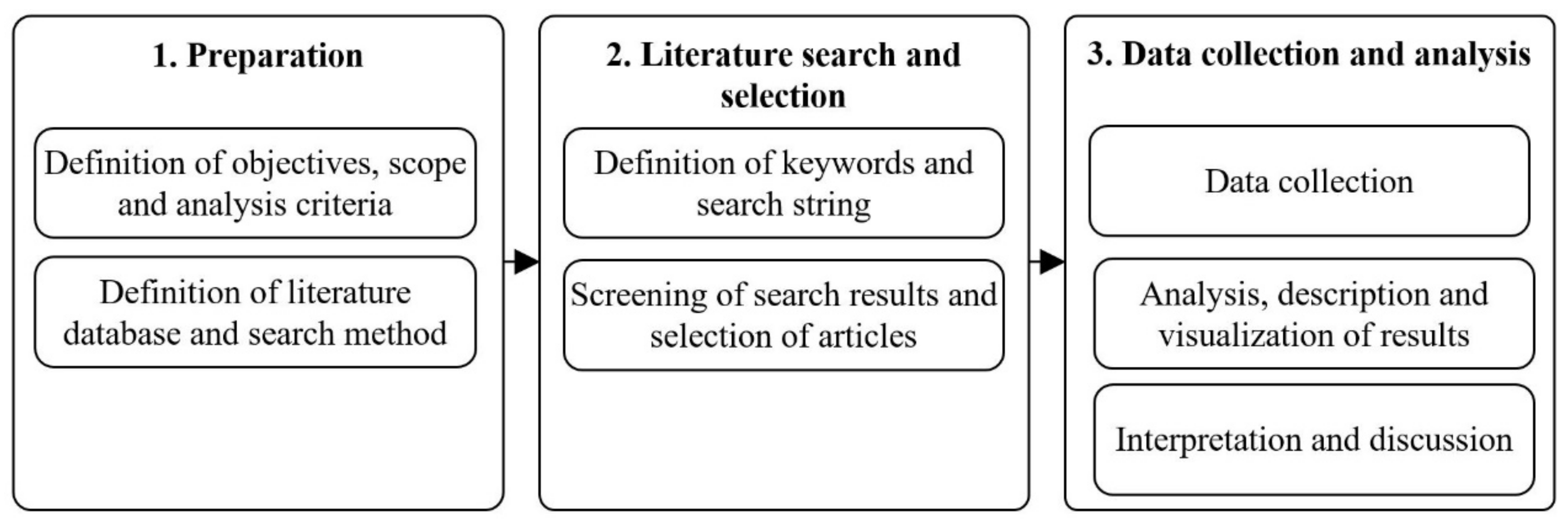
The literature review follows a systematic procedure as recommended in [4,7,9]. The step-by-step procedure is shown in Figure 1.

This review provides a comprehensive description and well-structured presentation of the content of recent international literature on energy demand modeling. Therefore, a systematic and replicable analysis of a high number of articles was conducted regarding the utilized techniques as well as associated input data, accuracy, and spatio-temporal resolution across different energy carriers and sectors. This comprehensive and concise literature classification serves as a decision-base for fellow researchers for the selection of appropriate data-model combinations for their projects. Direct and easy access to articles corresponding to a particular set of criteria is provided through structured tables in the Appendix A. Moreover, the advantages and drawbacks of common techniques as well as countermeasures against disadvantages are presented. This review constitutes an exploratory study examining and categorizing a broad and up-to-date literature base regarding an unprecedented number of properties using descriptive statistical methods. Challenges and future research directions are suggested and the compiled material provides a basis for future hypothesis-based quantitative testing.

The article is organized as follows: In Section 2, the systematic review process is described. In Section 3, a description and classification of techniques are given. In Section 4 the results of the literature analysis are presented, starting with sectors and energy carriers and followed by results on modeling techniques, input data, temporal and spatial characteristics as well as accuracy. In Section 5 most significant results are discussed and in Section 6 future research directions are suggested. The paper concludes with Section 7.

To aim for recent and relevant literature, the search was limited to articles published between 2015 and 2020 in journals related to energy, engineering, modeling, and simulation or computer science in English. The literature base for this review is the result of a replicable query to Web of Science Core Collection, a database for international journal publications and conference proceedings [15], on 1 May 2021. A search string was derived from a keyword matrix containing keywords from the thematic groups “energy”, “demand” and “modeling”. The search string and keyword matrix can be found in the Appendix A of this review (see

Table A2. Keyword compilation. The table contains the keywords used for the literature research arranged by thematic groups. Keywords in the bottom cell are explicitly excluded, which leads to a more precise search result. The * is a truncation operator to retrieve words with variant zero to many characters.

Energy	Demand	Modeling
Electric *	Demand	Forecast *
Natural gas	Consumption	Estimat *
Heat	Load	Predict *
	Requirement	Project *
	Intensity	Simulation
		Disaggregation
		Planning
		Model *
		Bottom-up
		Top-down
Excluded keywords: storage, carbon, emission, price, optimization, vehicle, climate
Search string applied to the Web of Science Core Collection on 1 May 2021: (TI = ((electric* OR “natural gas” OR heat) AND (demand OR consumption OR load OR requirement OR intensity) AND (forecast* OR estimat* OR predict* OR project* OR simulation OR disaggregation OR planning OR model* OR “bottom-up” OR “top-down”)) NOT TS = (storage OR carbon OR emission OR price OR optimization OR vehicle OR climate))

). The search yielded 695 articles, which were then further scrutinized based on their title and abstract resulting in an exclusion of 276 articles due to non-matching topics or closed access despite institutional logins at the publishers’ websites. The final literature collection contains 419 articles.

Articles are analyzed according to the properties listed in

Table 2. Assessment criteria. Overview of analysis criteria defining the collected data during step three of the review procedure. Each item represents a property characterizing the techniques applied in the respective articles. A short description and possible values are given. For mutually exclusive criteria only one value is possible, while for non-exclusive properties multiple values can be given and counted multiple times.

Analysis Criteria	Description	Possible Values	Mutually Exclusive
Technique	Modeling technique applied	Artificial neural network, support vector machine, regression, autoregressive methods, etc.	No
Category of techniques	General category of applied technique	Statistical, machine learning, metaheuristic, stochastic/fuzzy/grey, and engineering-based techniques	No
Technique combination	A single technique or a combination of techniques was applied	Stand-alone or hybrid approach	Yes
Model inputs	Inputs for energy demand models serving as explanatory variables and predictors	Data describing historic load, calendar information, weather, economy, demographics, environment, prices, behavior, and information about the technical system	No
Energy carrier	Forecasted/modeled type of energy	Electricity, natural gas, energy for heating and cooling	No
Sector	Economic sector or consumer group which is modeled	Industrial, commercial, residential, all sectors	No
Technical system	Applications or technical systems, which are modeled	Power grid, gas grid, district heating, building, production	No
Spatial resolution	Spatial level of detail of models	Country, regions (e.g., district), households/buildings, appliances	Yes
Temporal resolution	Scale of time steps that are described by the models	Sub-hourly, hourly, daily, above daily	Yes
Temporal horizon	Timespan that is covered by the models	Short-term (up to one day), medium-term (several weeks or months), long-term (one year and above)	Yes
Accuracy	Performance evaluation of presented models	Numeric values for MAPE	No

. Given the variety of entries for all the criteria, they have been grouped in the column “possible values” in Table 2. The spatial resolution is defined by the smallest energy-consuming entity, which is modeled in the respective articles. For the temporal horizon, various categorizations exist in the literature [4,16]. The chosen definition is inspired by Wei et al. [14]. The MAPE is defined as the average absolute discrepancy between the predicted value and the actual value, expressed as a percentage of the actual value [17]. It is a unitless performance measure and not dependent on the magnitude of the system, which makes it appropriate for comparing the performance of techniques applied in different contexts [18]. Therefore, it is a widely used accuracy measure in energy demand modeling [5]. For the techniques, a variety of classifications can be found in the literature. The following section provides a clear definition of categories of techniques used for energy demand modeling.

The 419 articles represent the total population of units whose properties are analyzed and described. Hence, descriptive statistical techniques are used in order to illustrate the frequency and contingency of the properties of the articles, using bar plots and box plots. The data collected from the articles are categorical in all cases except for the MAPE value, which is of numerical continuous type. For the MAPE value, a histogram was plotted in order to illustrate its (non-symmetric) distribution.

After classification and analysis, the results are presented using plots and structured tables for the direct accessibility of articles. Subsequently, highlights are discussed regarding particular advantages and drawbacks of techniques.

3. Classification of Techniques

A variety of classifications for techniques for energy demand modeling exists in the literature. Debnath and Mourshed [4] distinguish between statistical, computational intelligence (CI), and mathematical programming as well as stand-alone and hybrid techniques. Within the category of statistical techniques, they define regression, time series analysis (TSA), and autoregressive conditional heteroscedasticity (ARCH) techniques. Within the category of CI, they mention ML, uncertainty, and metaheuristic techniques as well as expert-based methods. Hong and Fang [5] suggest the two general categories of statistical and artificial intelligence techniques, with the former comprising multiple linear regression and TSA techniques and the latter including ANN, fuzzy regression, support vector machines (SVMs), and gradient boosting machines. Wei et al. [14] distinguish between conventional techniques, including TSA, regression, and grey models, and artificial intelligence techniques, such as ANN and SVM. Kuster et al. [9] discuss the categories of TSA, regression models, ANN, SVM, and bottom-up techniques.

This article is based on the classification by Debnath and Mourshed [4], however, extended by engineering-based techniques, which have been mentioned by other authors and referred to as bottom-up techniques [6,9,19,20,21,22]. Expert-based systems and mathematical programming mentioned in [4] are not considered since none of the analyzed articles followed either approach. Furthermore, the category of uncertainty techniques, which consists of fuzzy logic and grey models according to [4], is complemented by stochastic models, which have been encountered several times during data collection. The category name “uncertainty technique” might evoke some ambiguity amongst readers, since uncertainty is a natural property of any forecasting attempt. Therefore, the category is renamed “stochastic/fuzzy/grey systems theory”. Based on the classifications of [4,9] the following five categories are defined: statistical, ML, metaheuristic, stochastic/fuzzy/grey, and engineering-based techniques.

3.1. Statistical Techniques

According to [4,5], this category consists of regression and TSA techniques. As shown in [6], techniques from this category have been used in econometrics to explore the interrelationship between energy demand and economic development.

Regression techniques are used to solve an underlying regression problem [23], which consists of finding an approximation of a functional relation between numerical input and output variables. To find a solution for the approximation, different methods are employed, oftentimes minimizing the sum of the squares of errors [24]. For linear relations, this can be done by the ordinary least squares method. For non-linear relations, methods of steepest descent are used [24] or kernel functions [25]. Typical examples for statistical regression as found among the reviewed articles are linear, nonlinear, logistic, quantile, and ridge regression. Outside of statistical techniques, non-parametric regression can be found where ML techniques, such as ANN, kernel regression, or regression trees are employed to derive the functional form and regression parameters from the data [26,27].

TSA techniques derive their predictions from a historic time series, i.e., historic energy consumption data. In their core, many TSA approaches represent regression models since the predicted value is estimated based on one or more previous values [9]. This category includes univariate time series models such as autoregressive moving average (ARMA) models. Popular other techniques are autoregressive integrated moving average (ARIMA) models for non-stationary time series, seasonal autoregressive integrated moving average (SARIMA) models for seasonality, and ARMA models with exogenous variables (ARMAX) [5,28]. A typical multivariate TSA method is vector auto-regression as used in [29,30]. As suggested in [4], the category of TSA also includes exponential smoothing models and ARCH techniques.

3.2. Machine Learning Techniques

Techniques from this category find broad application in energy demand modeling and prediction and can be divided into supervised and unsupervised learning approaches.

Supervised learning approaches use labeled training datasets to derive a function describing a relation between inputs and outputs based on examples of input-output pairs [31]. They can be applied to numerical variables in the case of regression problems and categorical variables in the case of classification problems [32]. Within this sub-category, common techniques are ANN and instance-based algorithms, such as k-nearest neighbor and kernel machines [33]. A common example for the latter is SVM, which can convert nonlinear problems in low-dimensional space to linear problems in high-dimensional space [34]. Furthermore, in this category, there are decision trees, Bayesian algorithms, and ensemble learning approaches, such as gradient boosting machines [5].

Unsupervised learning approaches are often applied to clustering problems. These algorithms deduce structures in an unlabeled input dataset, e.g., through finding similarities [35].

3.3. Metaheuristic Techniques

Metaheuristic techniques oftentimes are used to solve optimization problems and can be incorporated into other techniques to improve performance [23]. The category includes evolutionary algorithms, which mimic mechanisms that are inspired by biological processes, such as reproduction, mutation, recombination, and selection [4]. It includes genetic algorithms, particle swarm optimization, bee colony optimization, firefly algorithms, and more [36]. In combination with ML approaches, they can be employed for parameter optimization in SVM [37] or weight optimization in ANN [22,38], resulting in approaches such as the firefly algorithm neural network [23]. Genetic algorithms are also used for feature selection in ML approaches [39,40].

3.4. Stochastic, Fuzzy and Grey Systems Theory Techniques

The techniques in this category are used to model different types of uncertainty. Zimmerman describes two basic forms of uncertainty: the traditional logic of probability describes randomness regarding the occurrence of an event, whereas fuzziness, describes the ambiguity of an event, i.e., to what extent an event occurs [41]. As Hájek et al. [42] point out, probability and fuzzy logic represent different sorts of uncertainty. Probability theory is used to describe stochastic processes [43] in which future states of a system are described by their past states plus a random change.

In energy demand modeling, stochastic processes such as Markov chains are used for forecasting and simulation of load profiles [20,44,45,46]. Fuzzy logic is employed in the form of fuzzy time series [47], fuzzy regression models [5], fuzzy clustering [48], and adaptive neuro-fuzzy interference systems (ANFIS) [49]. Tien states that fuzzy uncertainty can be analyzed with the grey system theory [50] and Debnath and Mourshed classify them as uncertainty methods [4]. The grey theory was proposed by Deng in 1982 and was developed to estimate the behavior of an uncertain system given only a limited amount of data [51]. The fundamental grey model GM(1,1) relies on as few as four recent data points to forecast the future data point [50]. The model uses the least square method to obtain the parameters for the grey differential equations, which describe the change between time steps [51].

3.5. Engineering-Based Techniques

Engineering-based techniques follow a bottom-up approach and use a variety of external and internal parameters to describe an energy-consuming system in high detail [6,23]. Oftentimes, individual loads of end-use appliances are considered to obtain aggregate profiles [19]. Common examples are models on the level of individual dwellings [52] or industrial processes [53] as well as building simulations [54]. Engineering-based models have proven their worth in planning and design of technical systems, being able to simulate a system’s behavior under conditions, for which there has been little historic data recorded yet [21]. Furthermore, they are promising approaches regarding the inclusion of the effects of household composition and individual behavior of dwellers as well as testing demand-side management strategies [20]. While techniques from this category are widely deployed in practice, they have been less visible in scientific articles on energy demand modeling and rarely been included in literature reviews.

Geographic information systems (GIS) are used for referencing data to geographic shapes, which have a distinct location and orientation relative to a reference coordinate system. Most of the time they are used for visualization and mapping of energy consumption as well as for urban [55] and rural [56] planning of infrastructure and building simulation [54,57].

4. Results

A total number of 419 articles originating from 54 different countries was reviewed. The country with the highest output of articles during the last years is China (98) followed by the USA (40) and Turkey (31). The analysis of the publication dates shows a slight increase of articles over the last six years from 66 in 2015 to 77 in 2020.

4.1. Sectors and Energy Carriers

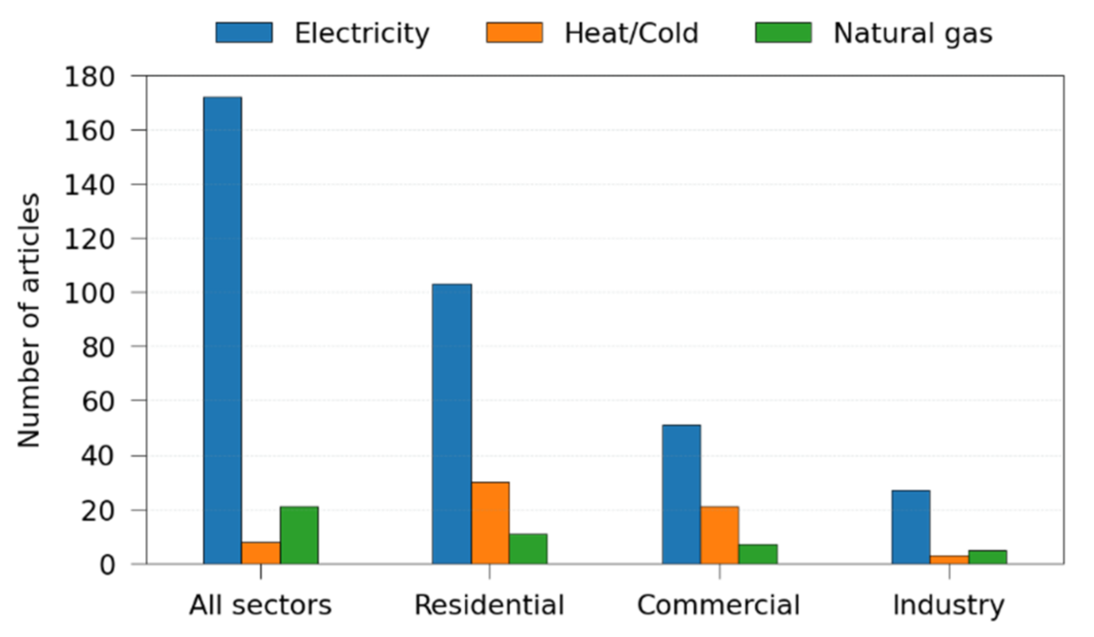
Figure 2 shows the energy carriers and economic sectors on which the articles were focused. It reveals that in most articles the consumer group is not limited to a single sector but rather comprises all sectors together. This is the case when the energy consumption of an entire (market-) region is modeled. However, targeted modeling of residential and commercial energy consumption is also common, while industrial consumers are analyzed rather rarely. A possible interpretation could be the lower availability of publicly available consumption data for the industrial sector compared to the other sectors. Moreover, industrial energy consumption tends to be less dependent on exogenous influencing factors (e.g., weather) and rather exhibits production-related temporal patterns that are difficult to predict without knowledge of internal processes, which can be company-specific and proprietary knowledge.

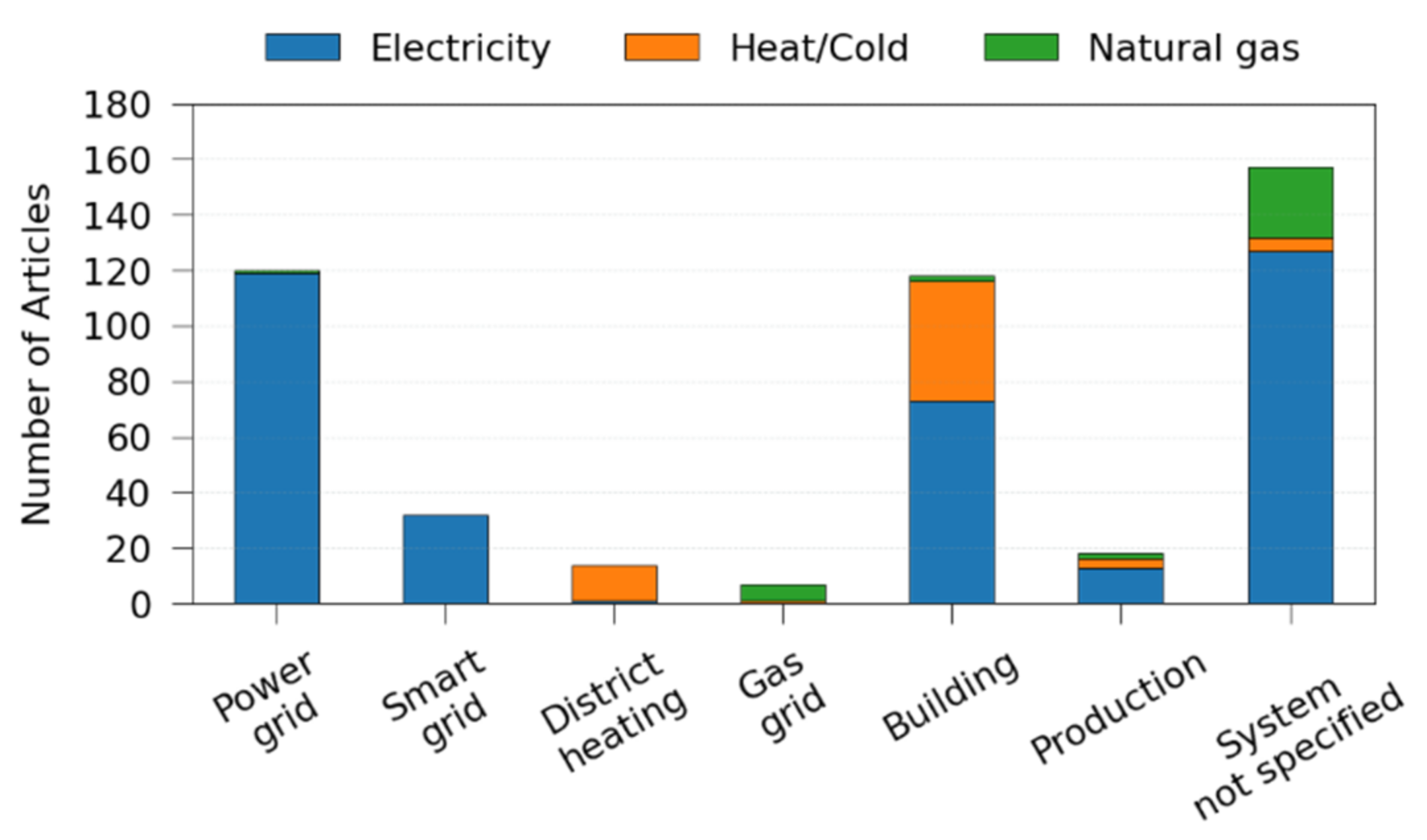
Figure 2 also shows that most articles focus on electricity demand. However, particularly within the residential and commercial sectors, various articles are modeling the consumption of thermal energy, i.e., demand for heating and cooling. This could be partially explained by the fact, that there is a significant number of articles focusing on energy in buildings in the residential and commercial sectors, where thermal energy accounts for the largest share of the energy consumed. A separate analysis of all technical systems showed that most articles focus on power grids, smart grids, and buildings (see Figure A3).

Table A3. Articles sorted by energy carrier and sector. A compilation of the results of the analysis regarding energy carriers and sectors, which allows for direct tracing of the respective references.

Energy Carrier	Sector	References
Electricity	All sectors	[5,16,27,29,30,33,34,39,40,47,48,51,52,58,59,60,69,70,71,72,73,81,82,88,89,90,94,95,97,100,103,105,106,108,109,110,111,113,117,118,129,135,136,138,139,140,141,142,147,148,149,157,161,162,163,165,168,169,170,172,176,177,178,179,181,182,184,185,186,189,190,191,202,203,225,226,227,228,229,230,231,232,233,234,235,236,237,238,239,240,241,242,243,244,245,246,247,248,249,250,251,252,253,254,255,256,257,258,259,260,261,262,263,264,265,266,267,268,269,270,271,272,273,274,275,276,277,278,279,280,281,282,283,284,285,286,287,288,289,290,291,292,293,294,295,296,297,298,299,300,301,302,303,304,305,306,307,308,309,310,311,312,313,314,315,316,317,318,319,320,321]
	Residential	[19,20,21,44,52,56,62,64,66,68,75,79,84,86,92,93,96,98,122,126,130,143,158,160,164,166,174,322,323,324,325,326,327,328,329,330,331,332,333,334,335,336,337,338,339,340,341,342,343,344,345,346,347,348,349,350,351,352,353,354,355,356,357,358,359,360,361,362,363,364,365,366,367,368,369,370,371,372,373,374,375,376,377,378,379,380,381,382,383,384,385,386,387,388,389,390,391,392,393]
	Commercial	[17,21,61,63,75,79,84,91,102,120,131,132,137,145,150,151,152,156,173,233,325,333,336,340,346,357,362,363,364,371,378,394,395,396,397,398,399,400,401,402,403,404,405,406,407,408,409,410,411,412,413]
	Industry	[45,49,51,53,79,84,155,180,226,233,249,336,351,362,371,408,414,415,416,417,418,419,420,421,422,423,424]
Gas	All sectors	[18,80,99,112,133,153,192,287,425,426,427,428,429,430,431,432,433,434,435,436]
	Residential	[104,116,437,438,439,440,441,442,443,444,445]
	Commercial	[83,104,116,137,438,441,443]
	Industry	[83,419,441,443,446]
Heating/cooling	All sectors	[37,87,146,175,183,447,448,449,450,451,452]
	Residential	[22,52,54,57,74,85,101,144,154,171,187,194,334,341,451,453,454,455,456,457,458,459,460,461,462,463,464]
	Commercial	[61,77,91,101,107,114,115,137,154,159,398,459,465,466,467,468,469,470,471,472,473]
	Industry	[53,419,474]

in Appendix A provides a structured reference list of the analyzed articles by energy carrier and sector. Fellow researchers can use this overview to find articles, which have similar objects of research with regard to the energy carriers and the sector.

4.2. Techniques and Input Data

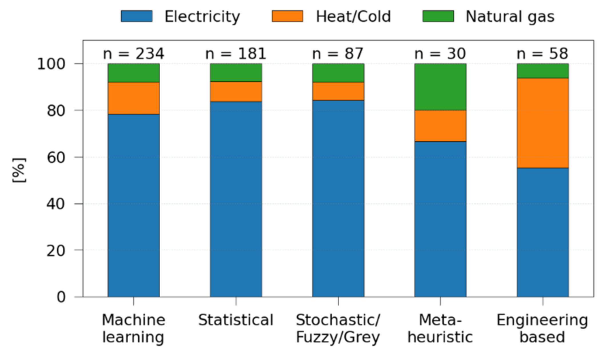
A variety of techniques is employed in the field of energy demand modeling. Figure 3 shows the number of appearances (n) of each of the five major categories of techniques (see Section 3) across all articles as well as the proportion of energy carriers whose consumption was modeled.

It is revealed that ML and statistical techniques are employed in most of the reviewed articles. A possible reason could be that ML and statistical techniques, like TSA, can be applied to a variety of use cases with relatively little effort in terms of model configuration and data preparation. They mainly require historic load data as input, which can be complemented by a limited set of external parameters, such as calendar or weather information [51,58,59,60]. Conventional regression techniques, like multiple linear regression, are commonly used among the articles as well and perform as benchmarks for other approaches [61,62,63].

Stochastic, fuzzy and grey techniques can be implemented as stand-alone models [64], e.g., simulating load profiles by sampling from stochastic processes such as Gaussian processes or Markov chains [52,65,66]. However, the representation of uncertain outcomes through stochastic, fuzzy or grey expressions is often combined with other techniques such as statistical regression [67,68] or ANN [69,70], giving results in the form of membership functions, intervals or probabilistic density.

Metaheuristic techniques are often used as part of hybrid techniques. Typical application is the optimization of model parameters [34,71] or feature selection [39,49] in ML models. Another example is the application of genetic algorithms in order to create optimized models as the result of an evolutionary process in which model a configuration is refined over multiple generations [72,73].

In the case of engineering-based techniques, energy demand is derived from the specifications of the system and its technical details [53,74,75]. Hence, an accurate simulation with an engineering-based model can require a high amount of data and effort, which might reduce the widespread use of such approaches [76]. However, engineering-based techniques are used to a greater extend to model heating and cooling demands, especially in the context of building simulation.

GIS techniques are used to reference data to geo-spatial shapes and visualization in the form of geographical maps. This has been used in the context of building simulation, where geometry and orientation was considered [54,57,77,78] or planning of rural [56] or urban [79,80] grid infrastructure. In other cases regional loads and trends in spatial energy consumption were analyzed [21,81,82,83] or modelled using socioeconomic data [84,85,86].

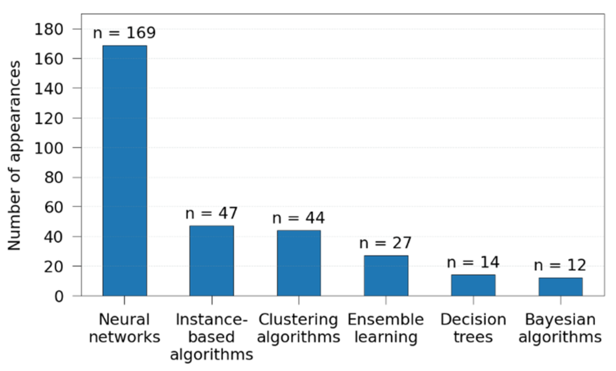
Figure 4 provides more details on the ML techniques that are used in the articles. ANNs [87,88], by far, show the highest number of appearances, followed by instance-based algorithms such as SVMs [89,90]. Clustering algorithms such as the k-means algorithm are used frequently to split datasets into groups of maximum similarity. This can be applied to the formation of consumer groups but also to finding similar days in historic load datasets [91,92,93]. Ensemble learning algorithms combine multiple ML techniques that are individually trained in order to obtain an improved overall performance. This can be achieved by bootstrap aggregating (bagging) [94,95] and boosting [96,97]. Bayesian algorithms and decision trees use supervised learning algorithms and therefore are typically used for regression and classification problems, e.g., Bayesian networks [98,99] or classification and regression trees [100,101]. By combining multiple decision trees through bagging, where each tree is trained on a different sub-sample of the dataset, random forest ensembles are created [94,102,103].

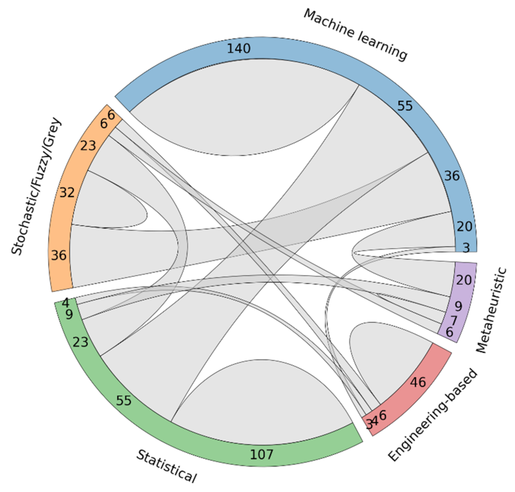
Overall, in 210 out of 419 articles a combined approach was employed. Figure 5 shows the combinations among the five main categories. The self-arcs show the number of times the respective technique was used as a stand-alone approach or was combined with a technique from the same category, which is the case for 63 articles within the category of ML, 17 articles with statistical techniques, three articles with metaheuristic techniques and respectively four articles with stochastic/fuzzy/grey and engineering-based techniques.

The analysis shows that among the analyzed articles, engineering-based techniques have the highest proportion of stand-alone models and metaheuristic techniques have the highest proportion of hybrid models. ML techniques often form hybrid techniques with themselves as well as with statistical and stochastic/fuzzy/grey techniques.

A typical example for a combined approach is the employment of techniques for clustering or frequency analysis for upstream data preparation. These techniques refine input data, e.g., by signal decomposition through Fourier or wavelet transformation, before the data is fed into a downstream model implemented by TSA [95,104,105] or ML techniques [106,107,108,109,110,111,112], where each of the decomposed signals is predicted separately. Another example is the integration of fuzzy mathematics into ANNs resulting in ANFIS [59,113,114,115] or the incorporation of metaheuristic optimization algorithms into the training stage of an ANN [116,117] or SVM [34,37,71].

In other cases, an overall prediction will be given as a weighted average of the results of multiple models, which can stem from different categories. The calculation of the weights can be subject to various (metaheuristic) optimization techniques, allowing TSA, regression or ML techniques to be combined into one approach [59,113,118,119,120]. In the case of engineering-based techniques, there are examples of combining simulation results from stochastic processes with bottom-up models, which are predominantly used for predicting energy demand in households [52,121,122].

Another aspect of the reviewed articles concerns the respective datasets that serve as inputs for the models.

Table 3. Model inputs. Classification of possible data-sets used as model input along with examples of data-sets.

Model Inputs	Examples
Historic energy demand	Historic load, electricity, heating, cooling, or natural gas demand
Weather data	Outside temperature, atmospheric pressure, cooling and heating degree days, humidity, solar radiation, wind speed
Calendar data	Time of day, day of the week, month, holidays, bridge days, seasons, workday, working hours, operating time of appliance
Demographic or economic data	Economic indicators: gross domestic product (GDP), gross national income (GNI), level of production, income, import and export level of a region; demographic indicators: human development indices, population, number of dwellers/buildings/residences, age, sex, education, infant mortality
Technical system data	Appliance data: equipment installed, number of appliances, efficiency, material properties, air change ratio, flow rate, outlet/inlet temperatures, rated power of the equipment, impedance Building data: floor space, number of bedrooms, transmission factor, building type, age of the building, efficiency rating, geometry of the building, the status of refurbishment, window area, building material, indoor temperature, indoor humidity
Usage and behavioral data	Time-use survey data, building usage (main residency, rented, owned, etc.), occupancy/activity patterns, operation/usage time of a device
Energy prices	Electricity and gas prices, tariffs, payment methods

gives an overview of examples for different model inputs, reflecting the variety of input data that is used in the field.

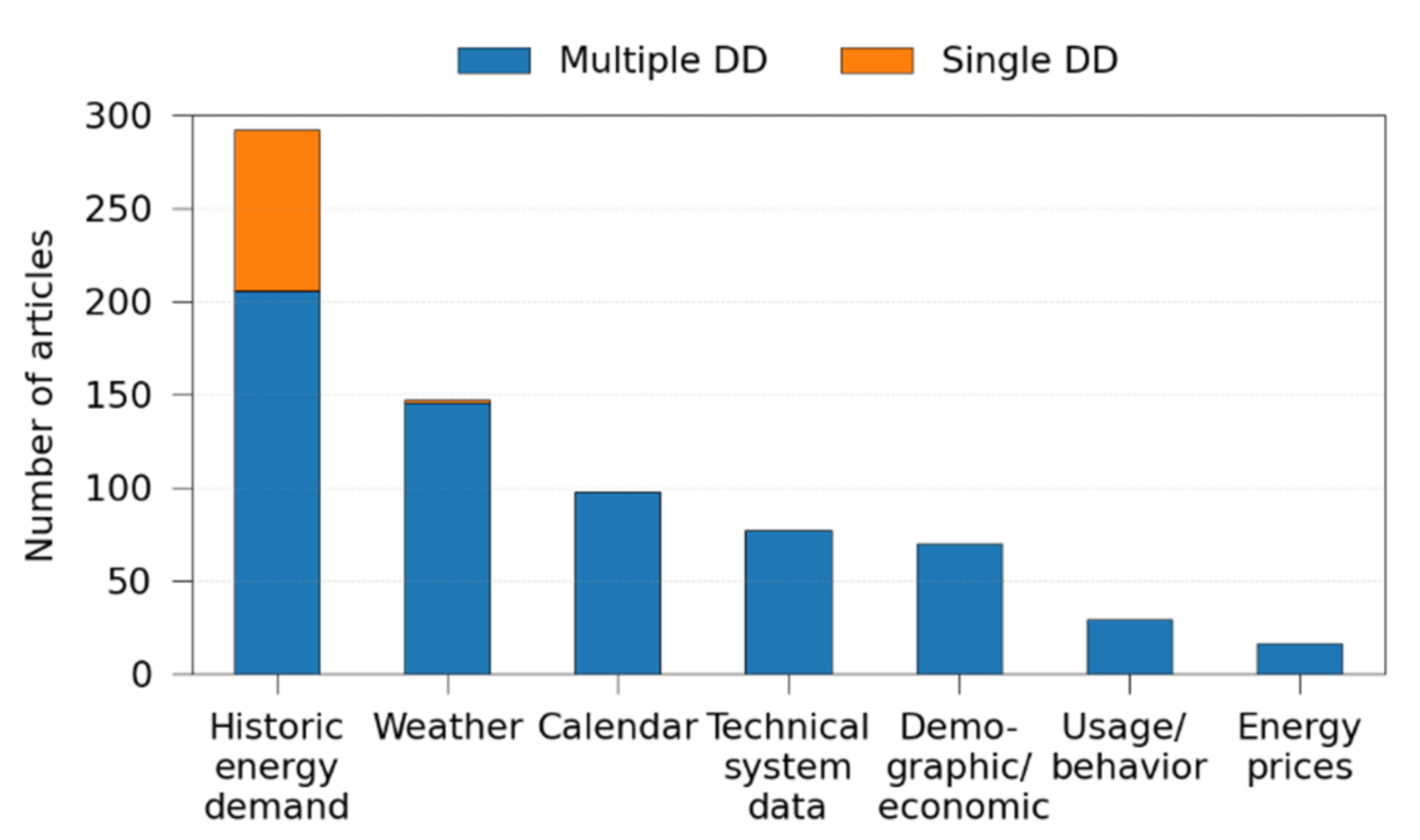
Figure 6 gives an overview of the frequency of usage of different types of input data as well as an indication of whether they are used in combination with others (“Multiple demand drivers (DD)”) or as a “single DD”. It is revealed that historic energy demand is used in 85% of the articles, which highlights its significance as a data source. As historic demand can be forecasted by trend extrapolation and pattern recognition, e.g., in the case of ARMA models, it constitutes a stand-alone data source.

Weather data is used in 43% of the articles. Its frequent use could be explained by the fact that operational patterns of some end-user devices are correlated with weather phenomena, e.g., heating, cooling, and lighting systems. Calendar information is also widely used (in 29% of the articles) since energy consumption can exhibit daily, weekly or annual patterns. For example, in most cases, the metering data of a company will reflect working hours.

Usage and behavioral data can be used to describe the relationship between energy consumption and user behavior, i.e., a parameter indicating that a technical device is now in use. Regional demographic and economic data describe properties of a region, such as household income or economic output, which can serve as predictors for the energy consumption of this region. The relatively rare use of price data might seem surprising, but can be explained by the international literature base largely covering countries with regulated or only recently liberalised energy markets, such as China, where price signals have not been transmitted to end consumers in the past [123]. Furthermore, energy demand has shown to be price inelastic both in the short and long-term [124], and therefore energy prices are not be considered as dominant drivers of demand.

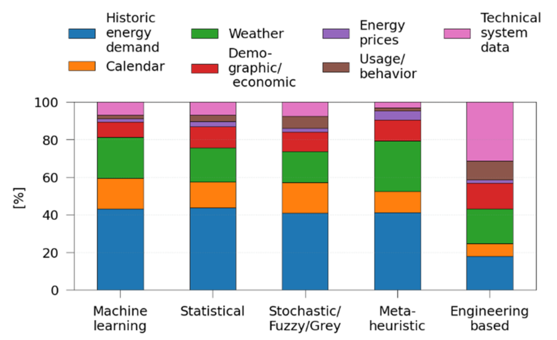
When taking a closer look at the usage of input data across the techniques (Figure 7), it becomes apparent that among the examined articles engineering-based techniques do not rely on historic energy demand data as much as the other techniques. Here, external parameters such as information on the technical system or weather data are essential, whereas historic energy demand is rather used for calibration and validation purposes.

Table 4. Techniques and input data used (1/5). Compiled results of the analysis on techniques and input data. Each cell provides a short assessment of the respective data-technique combination. The corresponding articles for each cell are documented in detail in the structured reference lists in Table A4, Table A5, Table A6 and Table A7 in Appendix A.

Technique	Advantages and Disadvantages of Techniques	Historic Energy Demand	Weather Data	Calendar Data	Demographic or Economic Data	Technical System Data	Usage or Behavioral Data	Energy Prices
ANN	+ Established for classification and regression problems (high performance), low effort, handle non-linear relations, big variety of pre-set models, no knowledge of technical system needed − Risk of over-fitting, difficult interpretation (black-box), feature engineering required	Contributions: 107 Impact: High; can be used as a single input Drawbacks: Outputs dependent on data quality and availability Outlook: Continuous intensive use	Contributions: 65 Impact: High; predictor for heating and cooling and lighting systems Drawbacks: Limited explanatory value for other applications than heating/cooling/ lighting Outlook: Continuous intensive use	Contributions: 44 Impact: High; Predictor for regular daily, weekly or annual patterns Drawbacks: Risk of overestimation of periodic routines, cannot account for special events without knowledge Outlook: Continuous intensive use	Contributions: 13 Impact: Low for short-term load prediction; high for long-term regional, sectoral, or national demand prediction Drawbacks: Low level of detail regarding individual consumer patterns, usually yearly or quarterly resolution Outlook: Continuous use in cases of long-term national or sectoral demand modeling	Contributions: 18 Impact: High; explanatory value regarding process internal and end-user devices Drawbacks: Difficult to collect, have to be measured using sensors, might be subject to data privacy or company secrets Outlook: Occasional use, could see intensification	Contributions: 6 Impact: Potentially high; explanatory value regarding individual consumer patterns Drawbacks: High effort to collect because the result of time-of- use surveys, subject to privacy or company secrets, difficult to predict, the output of simulations Outlook: Rare use, could see intensification	Contributions: 4 Impact: Low Drawbacks: Rarely considered as a predictor because demand has low price elasticity, price swings only in liberalized markets, difficult to obtain future values to use in predictions Outlook: Rare use
Instance-based	+ Established for classification problems, good performance with a high number of features, for kernel machines there are many pre-set kernel functions to choose from, transforms nonlinear relations into linear ones in the feature space, robust against overfitting − Medium/high effort, dependent on the right choice of kernel, memory-intensive and limited scalability for big datasets	Contributions: 35 Impact: High; usually complemented by additional features Drawbacks: Outputs dependent on data quality and availability Outlook: Continuous intensive use	Contributions: 19 Impact: High; predictor for heating and cooling and lighting systems Drawbacks: Limited explanatory value for other applications than heating/cooling/lighting Outlook: Continuous intensive use	Contributions: 15 Impact: High; Predictor for regular daily, weekly or annual patterns Drawbacks: Risk of overestimation of periodic routines, cannot account for special events without knowledge Outlook: Continuous intensive use	Contributions: 11 Impact: High for classification of regions or consumer groups; low for short-term load prediction Drawbacks: Low level of detail regarding individual consumer patterns, usually yearly or quarterly resolution Outlook: Continuous use in cases of regional or sectoral modeling	Contributions: 8 Impact: High; explanatory value regarding process internal and end-user devices Drawbacks: Difficult to collect, have to be measured using sensors, might be subject to data privacy or company secrets Outlook: Occasional use, could see intensification	Contributions: 0 Impact: Potentially high explanatory value for classification of typical time steps considering individual consumer patterns Drawbacks: High effort to collect because the result of time-of- use surveys, subject to privacy or company secrets, difficult to predict, the output of simulations Outlook: No use, could see intensification	Contributions: 2 Impact: Low Drawbacks: rarely considered as a predictor because demand has low price elasticity, price swings only in liberalized markets, difficult to obtain future values to use in predictions Outlook: Rare use
Clustering	+ Finding natural groupings in an unsupervised learning process, easy to implement, different algorithms in place based on geographic distance (K-means), graph distance (affinity propagation), density (DBSCAN), or a hierarchical approach − Assumptions on the number and shape of clusters can be necessary and lead to mistakes	Contributions: 34 Impact: High; used to find similar time steps or similar consumer groups Drawbacks: Outputs dependent on data quality and availability Outlook: Continuous intensive use	Contributions: 13 Impact: High; used for finding similar days, a predictor for heating and cooling and lighting systems Drawbacks: Limited explanatory value for other applications than heating/cooling/ lighting Outlook: Continuous intensive use	Contributions: 12 Impact: High; for regular daily, weekly or annual patterns Drawbacks: Risk of overestimation of periodic routines, cannot account for special events without knowledge Outlook: Continuous intensive use	Contributions: 9 Impact: High for classification of regions or consumer groups; low for short-term load prediction; Drawbacks: Low level of detail regarding individual consumer patterns, usually yearly or quarterly resolution Outlook: Continuous use in cases of regional or sectoral modeling	Contributions: 5 Impact: High; explanatory value regarding process internal and end-user devices Drawbacks: Difficult to collect, have to be measured using sensors, might be subject to data privacy or company secrets Outlook: Occasional use, could see intensification	Contributions: 2 Impact: Potentially high explanatory value for classification of typical time steps considering individual consumer patterns Drawbacks: High effort to collect because the result of time-of- use surveys, subject to privacy or company secrets, difficult to predict, the output of simulations Outlook: Rare use, could see intensification	Contributions: 1 Impact: Low Drawbacks: Rarely considered as a predictor because demand has low price elasticity, price swings only in liberalized markets, difficult to obtain future values to use in predictions Outlook: Rare use

,

Table 5. Techniques and input data used (2/5).

Technique	Advantages and Disadvantages of Techniques	Historic Energy Demand	Weather Data	Calendar Data	Demographic or Economic Data	Technical System Data	Usage or Behavioral Data	Energy Prices
Ensemble learning	+ Improved predictive performance by combi-ning the predictions of multiple models, in-creased robustness by reducing the variance of prediction errors − Requires additional knowledge to solve the bias-variance tradeoff	Contributions: 19 Impact: High; always used Drawbacks: Outputs dependent on data quality and availability Outlook: Continuous use	Contributions: 12 Impact: High; predictor for heating and cooling and lighting systems Drawbacks: Limited explanatory value for other applications than heating/cooling/ lighting Outlook: Continuous use	Contributions: 9 Impact: High; Predictor for regular daily, weekly or annual patterns Drawbacks: Risk of overestimation of periodic routines, cannot account for special events without knowledge Outlook: Continuous use	Contributions: 1 Impact: Low for short-term load prediction; high for long-term regional, sectoral, or national demand prediction, Drawbacks: Low level of detail regarding individual consumer patterns, usually yearly or quarterly resolution Outlook: Use in cases of regional or sectoral modeling	Contributions: 3 Impact: Potentially high; explanatory value regarding process internal and end-user devices Drawbacks: Difficult to collect, have to be measured using sensors, might be subject to data privacy or company secrets Outlook: Occasional use, could see intensification	Contributions: 1 Impact: Potentially high; explanatory value regarding individual consumer patterns Drawbacks: a high effort to collect because the result of time-of-use surveys, subject to privacy or company secrets, difficult to predict, the output of simulations Outlook: Rare use, could see intensification	Contributions: 1 Impact: Low Drawbacks: Rarely considered as a predictor because demand has low price elasticity, price swings only in liberalized markets, difficult to obtain future values to use in predictions Outlook: Rare use
Deep learning	+ Established for classification and regression problems, can learn complex patterns be using hidden layers creating intermediary representations of the data, reduced need for feature engineering using drop-out layers − Large amounts of training data required, specialized algorithms, computationally intensive to train, require additional expertise to tune	Contributions: 17 Impact: High; always used Drawbacks: Outputs dependent on data quality and availability Outlook: Continuous use	Contributions: 9 Impact: High; often used for short term load forecasting Drawbacks: Limited explanatory value for other applications than heating/ cooling/lighting Outlook: Continuous use	Contributions: 7 Impact: High; Predictor for regular daily, weekly or annual patterns Drawbacks: Risk of overestimation of periodic routines, cannot account for special events without knowledge Outlook: Continuous use	Contributions: 1 Impact: Low for short-term load prediction; high for long-term regional, sectoral, or national demand prediction Drawbacks: Low level of detail regarding individual consumer patterns, usually yearly or quarterly resolution Outlook: Use in cases of regional or sectoral modeling	Contributions: 1 Impact: Potentially high; explanatory value regarding process internal and end-user devices Drawbacks: Difficult to collect, have to be measured using sensors, might be subject to data privacy or company secrets Outlook: Rare use, could see intensification	Contributions: 1 Impact: Potentially high; explanatory value regarding individual consumer patterns Drawbacks: High effort to collect because the result of time-of-use surveys, subject to privacy or company secrets, difficult to predict, the output of simulations Outlook: Rare use, could see intensification	Contributions: 0 Impact: Low Drawbacks: Rarely considered as a predictor because demand has low price elasticity, price swings only in liberalized markets, difficult to obtain future values to use in predictions Outlook: No use
Bayesian algorithms	+ Established for classification, basic models (Naïve Bayes) have low implementation effort, good performance, good scalability, are able to handle conflicting/limited information and nonlinear relations − Design of advanced models (B. networks) requires expert knowledge or good data to learn from, computationally expensive, therefore simplifications are used, however, they assume conditional independence between input features, which is rarely true	Contributions: 9 Impact: High if used for forecasting Drawbacks: Outputs dependent on data quality and availability Outlook: Continuous use	Contributions: 8 Impact: High; used in almost all cases, often used for forecasting for heating and cooling demand Drawbacks: Limited explanatory value for other applications than heating/ cooling/lighting Outlook: Continuous use	Contributions: 5 Impact: High; used in short-term forecasts, Predictor for regular daily, weekly or annual patterns Drawbacks: Risk of overestimation of periodic routines, cannot account for special events without knowledge Outlook: Continuous use	Contributions: 2 Impact High for classification of regions or consumer groups; low for short-term load prediction; Drawbacks: Low level of detail regarding individual consumer patterns, usually yearly or quarterly resolution Outlook: Use in cases of regional or sectoral modeling	Contributions: 2 Impact: Low for forecasting, used in cases of algorithms for energy management and system control Drawbacks: Difficult to collect, have to be measured using sensors, might be subject to data privacy or company secrets Outlook: Sporadic use	Contributions: 1 Impact: Low for forecasting; potentially high for classification of typical time steps considering individual consumer patterns, used for simulations of demand in smart grids Drawbacks: High effort to collect because the result of time-of-use surveys, subject to privacy or company secrets, difficult to predict, the output of simulations Outlook: Rare use	Contributions: 1 Impact: Low, can be used for simulation of smart grids Drawbacks: Rarely considered as a predictor because demand has low price elasticity, price swings only in liberalized markets, difficult to obtain future values to use in predictions Outlook: Rare use

,

Table 6. Techniques and input data used (3/5). Continuation of Table 5.

Technique	Advantages and Disadvantages of Techniques	Historic Energy Demand	Weather Data	Calendar Data	Demographic or Economic Data	Technical System Data	Usage or Behavioral Data	Energy Prices
Decision trees	+ Established for classification, rarely used for regression, handles non-linear relationships by splitting data into homogenous sub-samples, low effort in data preparation, robust to outliers or missing values, good scalability − Risk of overfitting, very data sensitive, a small change in data can result in a major change of tree structure	Contributions: 7 Impact: High; always used Drawbacks: Outputs dependent on data quality and availability Outlook: Continuous use	Contributions: 5 Impact: High; used in almost all cases, often used for forecasting for heating and cooling demand Drawbacks: Limited explanatory value for other applications than heating/ cooling/lighting Outlook: Continuous use	Contributions: 5 Impact: High; used in short-term forecasts, a predictor for regular daily, week-ly or annual patterns Drawbacks: Risk of overestimation of periodic routines, cannot account for special events without knowledge Outlook: Continuous use	Contributions: 3 Impact: High for classification of regions or consumer groups; low for short-term load prediction; Drawbacks: Low level of detail regarding individual consumer patterns, usually yearly or quarterly resolution Outlook: Continuous use in cases of regional or sectoral modeling	Contributions: 3 Impact: High; explanatory value regarding process internal and end-user devices Drawbacks: Difficult to collect, have to be measured using sensors, might be subject to data privacy or company secrets Outlook: Occasional use, could see intensification	Contributions: 0 Impact: Potentially high; explanatory value for classification of typical time steps considering individual consumer patterns Drawbacks: High effort to collect because the result of time-of-use surveys, subject to privacy or company secrets, difficult to predict, the output of simulations, Outlook: Could see intensification	Contributions: 0 Impact: Low Drawbacks: Rarely considered as a predictor because demand has low price elasticity, price swings only in liberalized markets, difficult to obtain future values to use in predictions Outlook: Rare use
Regression	+ Low implementation effort, good performance, computationally inexpensive, white box character, measures against overfitting in place (regularization) − Risk of underfitting, sensitive to outliers, the underlying assumption that features are independent does not hold in reality	Contributions: 88 Impact: High; the dependent variable Drawbacks: Outputs dependent on data quality and availability Outlook: Continuous intensive use	Contributions: 50 Impact: High; one of the most used independent variables, especially for heating/ cooling/lighting Drawbacks: Limited explanatory value for other applications than heating/cooling/lighting Outlook: Continuous intensive use	Contributions: 31 Impact: High; predictor for regular daily, weekly or annual patterns Drawbacks: Risk of overestimation of periodic routines, cannot account for special events without knowledge Outlook: Continuous intensive use	Contributions: 31 Impact: High for long-term regional, sectoral or national demand prediction Drawbacks: Low level of detail regarding individual consumer properties, usually yearly or quarterly resolution Outlook: Continuous intensive use in cases of regional or sectoral modeling	Contributions: 13 Impact: High; explanatory value regarding process internal and end-user devices Drawbacks: Difficult to collect, have to be measured using sensors, might be subject to data privacy or company secrets Outlook: Occasional use, could see intensification	Contributions: 10 Impact: Potentially high; explanatory value regarding individual consumer patterns Drawbacks: High effort to collect because the result of time-of-use surveys, subject to privacy or company secrets, difficult to predict, the output of simulations Outlook: Occasional use, could see intensification	Contributions: 3 Impact: Low Drawbacks: Rarely considered as a predictor because demand has low price elasticity, price swings only in liberalized markets, difficult to obtain future values to use in predictions Outlook: Rare use
TSA/ARCH	+ Low implementation effort, data cleaning, and understanding is done at the same time, uncovers patterns in data like autocorrelation and seasonality, filters out noise, lots of pre-set models − Cannot predict unpreceded events, poor handling of outliers which can be propagated into future, not many techniques to deal with large numbers of variables and complex relationships, less suitable for long-term forecasting	Contributions: 78 Impact: High; always used, often used as a single input Drawbacks: Outputs dependent on data quality and availability Outlook: Continuous intensive use	Contributions: 20 Impact: Medium; used as an external variable, especially for heating/cooling/ lighting Drawbacks: Limited explanatory value for other applications than heating/cooling/lighting Outlook: Continuous use	Contributions: 19 Impact: Medium; used as an external variable, a predictor for regular temporal patterns Drawbacks: Risk of overestimation of periodic routines, cannot account for special events without knowledge Outlook: Continuous use	Contributions: 10 Impact: Low for short-term load prediction; medium for long-term regional, sectoral, or national demand prediction Drawbacks: Low level of detail regarding individual consumer patterns, usually yearly or quarterly resolution Outlook: Use in cases of regional or sectoral modeling	Contributions: 0 Impact: Low; use of many external variables is generally rare with TSA Drawbacks: Difficult to collect, have to be measured using sensors, might be subject to data privacy or company secrets Outlook: Rare use	Contributions: 1 Impact: Low; use of many external variables is generally rare with TSA Drawbacks: High effort to collect because the result of time-of-use surveys, subject to privacy or company secrets, difficult to predict, the output of simulations Outlook: Rare use	Contributions: 1 Impact: Low; since external variables are generally rarely used with TSA in general Drawbacks: Rarely considered as a predictor because of low price elasticity, price swings only in liberalized markets, difficult to obtain future values Outlook: Rare use

,

Table 7. Techniques and input data used (4/5). Continuation of Table 6.

Technique	Advantages and Disadvantages of Techniques	Historic Energy Demand	Weather Data	Calendar Data	Demographic or Economic Data	Technical System Data	Usage or Behavioral Data	Energy Prices
Stochastic	+ Capacity to handle uncertainty regarding the occurrence of events and produce variations of possible outcomes, the underlying assumptions about the randomness can be tested statistically, allowing to estimate not only the expected value but also the variations of the expected values Potentially high implementation effort can be computationally expensive, results can be difficult to communicate	Contributions: 33 Impact: High; used to define probability distribution on historic values Drawbacks: Outputs dependent on data quality and availability Outlook: Continuous intensive use	Contributions: 15 Impact: High; predictor for heating and cooling and lighting systems Drawbacks: Limited explanatory value for other applications than heating/cooling/lighting Outlook: Continuous intensive use	Contributions: 15 Impact: High; predictor for regular daily, weekly or annual patterns Drawbacks: Risk of overestimation of periodic routines, cannot account for special events without knowledge Outlook: Continuous intensive use	Contributions: 10 Impact: High for long-term regional, sectoral or national demand prediction Drawbacks: Low level of detail regarding individual consumer properties, usually yearly or quarterly resolution Outlook: Continuous intensive use in cases of regional or sectoral modeling	Contributions: 8 Impact: High; explanatory value regarding process internal and end-user devices Drawbacks: Difficult to collect, have to be measured using sensors, might be subject to data privacy or company secrets Outlook: Continuous use, could see intensification	Contributions: 8 Impact: High; explanatory value regarding individual consumer patterns Drawbacks: High effort to collect because the result of time-of-use surveys, subject to privacy or company secrets, difficult to predict, the output of simulations Outlook: Continuous use, could see intensification	Contributions: 2 Impact: Low; can be used for simulation of smart grids Drawbacks: Rarely considered as a predictor because demand has low price elasticity, price swings only in liberalized markets, difficult to obtain future values to use in predictions Outlook: Sporadic use
Fuzzy	+ Adopts vagueness in human reasoning modeling the degree of occurrence of an event, can display a range of possibilities for inputs by applying membership functions (fuzzyfication), can handle incomplete data, after the model’s ruleset is applied defuzzyfication can be done following different principles (e.g., weighted average), computationally inexpensive, − Results can be perceived as inaccurate, communication of results can be difficult, depends on expert knowledge to be set up, extensive validation and testing	Contributions: 32 Impact: High; exact usage also depends on the other part of the hybrid model (ML, TSA, etc.) Drawbacks: Outputs dependent on data quality and availability Outlook: Continuous intensive use	Contributions: 11 Impact: High; predictor for heating and cooling and lighting systems Drawbacks: Limited explanatory value for other applications than heating/cooling/lighting Outlook: Continuous intensive use	Contributions: 10 Impact: Medium; exact usage depends on an-other part of the hybrid model, usually no fuzziness about calendar information Drawbacks: Risk of overestimation of periodic routines, cannot account for special events without knowledge Outlook: Continuous use	Contributions: 7 Impact: High for long-term regional, sectoral or national demand prediction Drawbacks: Low level of detail regarding individual consumer properties, usually yearly or quarterly resolution Outlook: Continuous intensive use in cases of regional or sectoral modeling	Contributions: 3 Impact: Medium; exact usage depends on another part of the hybrid model, high explanatory value regarding process internal and end-user devices Drawbacks: Difficult to collect, have to be measured using sensors, might be subject to data privacy or company secrets Outlook: Occasional use, could see intensification	Contributions: 2 Impact: Potentially high; explanatory value regarding individual consumer patterns Drawbacks: High effort to collect because the result of time-of-use surveys, subject to privacy or company secrets, difficult to predict the output of simulations Outlook: Occasional use, could see intensification	Contributions: 1 Impact: Low; can be used for simulation of smart grids Drawbacks: Rarely considered as a predictor because demand has low price elasticity, price swings only in liberalized markets, difficult to obtain future values to use in predictions Outlook: Sporadic use
Metaheuristic	+ Provide alternative and promising algorithms to solve optimization problems and efficiently search the solution space, variety of metaheuristic algorithms in place which requires little implementation effort − No guarantee that the global maximum is attained, selection of algorithm can be difficult, depending on adequate parameter tuning	Contributions: 26 Impact: High; exact usage also depends on the other part of the hybrid model (ML, regression, etc.) Drawbacks: Outputs dependent on data quality and availability Outlook: Continuous intensive use	Contributions: 17 Impact: high, often used as a predictor for heating/cooling/lighting Drawbacks: Limited explanatory value for other applications than heating/cooling/lighting Outlook: Continuous intensive use	Contributions: 7 Impact: Medium; exact usage depends on an-other part of the hybrid model Drawbacks: Risk of overestimation of periodic routines, cannot account for special events without knowledge Outlook: Continuous use	Contributions: 7 Impact: High for long-term regional, sectoral or national demand prediction Drawbacks: Low level of detail regarding individual consumer properties, usually yearly or quarterly resolution Outlook: Continuous intensive use in cases of regional or sectoral modeling	Contributions: 2 Impact: Potentially high; explanatory value regarding process internal and end-user devices, exact usage depends on another part of the hybrid model Drawbacks: Difficult to collect, have to be measured using sensors, might be subject to data privacy or company secrets Outlook: Occasional use, could see intensification	Contributions: 1 Impact: Potentially high; explanatory value regarding individual consumer patterns Drawbacks: High effort to collect because the result of time-of-use surveys, subject to privacy or company secrets, difficult to predict, the output of simulations Outlook: Rare use, could see intensification	Contributions: 3 Impact: Low Drawbacks: Rarely considered as a predictor because demand has low price elasticity, price swings only in liberalized markets, difficult to obtain future values to use in predictions Outlook: Occasional use

and

Table 8. Techniques and input data used (5/5). Continuation of Table 7.

Technique	Advantages and Disadvantages of Techniques	Historic Energy Demand	Weather Data	Calendar Data	Demographic or Economic Data	Technical System Data	Usage or Behavioral Data	Energy Prices
Engineering-based	+ White box character, revealing detailed input-output relations, Able to simulate energy demand for explorative and normative scenarios including disruptions that have no historic record − Data and knowledge-intensive, prediction accuracy can be low due to simplifications regarding the system	Contributions: 21 Impact: High; historic demand used for validation of model outputs Drawbacks: Outputs dependent on data quality and availability Outlook: Continuous intensive use	Contributions: 22 Impact: high, often used as a predictor for heating/cooling/lighting Drawbacks: Limited explanatory value for other applications than heating/cooling/lighting Outlook: Continuous intensive use	Contributions: 8 Impact: Medium; not needed to describe physical input-output relations, a predictor for regular daily, weekly or annual patterns Drawbacks: Risk of overestimation of periodic routines, cannot account for special events without know-ledge Outlook: Continuous use	Contributions: 16 Impact: High for long-term regional, sectoral or national demand prediction Drawbacks: Low level of detail regarding individual consumer properties, usually yearly or quarterly resolution Outlook: Continuous intensive use in cases of regional or sectoral modeling	Contributions: 37 Impact: High; most important information to describe physical input-output relations, Drawbacks: High amount of data needed, difficult to collect, have to be measured using sensors, might be subject to data privacy or company secrets Outlook: Continuous intensive use	Contributions: 12 Impact: Potentially high; explanatory value regarding individual consumer patterns Drawbacks: High effort to collect because the result of time-of-use surveys, subject to privacy or company secrets, difficult to predict, the output of simulations Outlook: Continuous use, could see intensification	Contributions: 2 Impact: Low Drawbacks: Rarely considered as a predictor, not needed for physical input-output relations, demand has low price elasticity, price swings only in liberalized markets, difficult to obtain future values to use in predictions Outlook: Rare use

present the results of the analysis on the techniques and inputs used in the examined articles. They allow the reader to directly identify the compatibility of the data spectrum and methodology. The first two columns contain the techniques and associated advantages and disadvantages. The other columns refer to the input data types. In each cell a short assessment of the respective data-technique combination in the context of energy demand modeling is given in the following categories:

• “Contributions” refers to the number of relevant articles.
• “Impact” describes the importance (high, medium, low) of the data type for the respective technique considering different use-cases.
• “Drawbacks” refers to the weaknesses and limitations of the data-technique combination.

“Outlook” gives a qualitative assessment of the applicability in future research based on the number of contributions and the rating on impact and drawbacks, revealing possible research fields with high or limited potential for application.

All articles relevant for each cell, are documented in detail in the structured reference lists in

Table A4. Techniques and input data used per article (1/4) (thanks to the reviewers’ advice, Table 5, Table 6, Table 7, Table 8 and Table 9 have been designed in a clear and understandable structure, highlighting techniques and applications).

Method	Input	References
ANN	Historic energy demand	[16,21,40,45,48,49,51,58,59,60,68,69,70,72,73,80,82,87,88,91,94,96,97,99,100,101,106,108,110,112,113,114,115,116,117,118,130,131,132,135,136,137,138,145,146,147,148,153,154,159,161,162,164,165,166,167,168,172,173,174,176,184,185,191,229,235,237,244,248,249,252,255,260,261,263,265,267,270,277,278,283,286,288,293,294,325,340,342,346,348,349,352,354,356,360,363,366,373,399,402,405,407,427,428,442,448,453,454,456,470,475,476,477]
	Weather data	[21,22,40,68,69,70,80,82,87,91,96,97,101,106,112,114,115,118,130,132,136,138,145,146,147,148,151,153,154,159,164,165,172,173,174,176,183,191,229,237,244,255,261,263,267,275,325,340,348,349,356,363,402,405,407,427,432,442,448,454,456,470,476,477]
	Calendar data	[48,70,73,88,94,97,99,101,106,110,112,113,114,115,118,136,138,146,147,154,159,162,164,165,173,183,184,185,229,235,237,244,263,293,325,340,342,348,349,354,399,470,477]
	Demographic or economic data	[21,40,49,82,101,133,148,255,258,270,277,348,356]
	Technical system data	[22,68,80,82,87,91,96,101,144,159,269,354,366,402,416,453,457,474]
	Usage or behavioral data	[40,96,151,255,348,432]
	Energy prices	[49,96,148,427]
Instance based	Historic energy demand	[33,34,37,39,68,71,82,89,90,101,107,108,111,131,147,163,175,178,229,236,263,285,331,340,346,349,356,361,365,396,398,425,442,449,478]
	Weather data	[37,39,68,82,89,101,107,147,163,175,183,229,263,340,349,356,396,442,449]
	Calendar data	[39,101,111,147,183,229,236,263,331,340,349,396,425,449,478]
	Demographic or economic data	[34,82,89,101,107,178,258,285,331,356,478]
	Technical system data	[37,68,82,101,107,398,449,457]
	Usage or behavioral data	n/a
	Energy prices	[178,331]

,

Table A5. Techniques and input data used per article (2/4). Continuation of Table A4.

Method	Input	References
Clustering	Historic energy demand	[21,48,49,81,82,91,92,93,109,114,118,155,163,232,234,235,236,263,268,279,322,323,326,328,342,353,355,360,369,372,395,403,428,476]
	Weather data	[21,82,91,92,93,114,118,163,263,275,348,353,476]
	Calendar data	[48,92,93,109,114,118,235,236,263,326,342,348]
	Demographic or economic data	[21,49,81,82,93,232,234,348,395]
	Technical system data	[82,91,93,353,395]
	Usage or behavioral data	[348,395]
	Energy prices	[49]
Ensemble learning	Historic energy demand	[94,95,96,97,100,106,114,120,130,132,133,138,162,168,355,363,407,449,476]
	Weather data	[95,96,97,106,114,130,132,138,363,407,449,476]
	Calendar data	[94,95,97,106,114,120,138,162,449]
	Demographic or economic data	[133]
	Technical system data	[96,144,449]
	Usage or behavioral data	[96]
	Energy prices	[96]
Deep learning	Historic energy demand	[21,72,73,106,153,164,165,166,167,229,248,267,278,293,325,352,366]
	Weather data	[21,106,153,164,165,229,267,325,432]
	Calendar data	[73,106,164,165,229,293,325]
	Demographic or economic data	[21]
	Technical system data	[366]
	Usage or behavioral data	[432]
	Energy prices	n/a
Bayesian algorithms	Historic energy demand	[39,98,99,145,146,164,249,250,405]
	Weather data	[39,98,145,146,164,239,345,405]
	Calendar data	[39,98,146,164,239]
	Demographic or economic data	[99,345]
	Technical system data	[269,345]
	Usage or behavioral data	[98]
	Energy prices	[98]
Decision trees	Historic energy demand	[100,101,228,407,446,449,468]
	Weather data	[101,407,446,449,468]
	Calendar data	[101,228,446,449,468]
	Demographic or economic data	[101,446,468]
	Technical system data	[101,457,468]
	Usage or behavioral data	n/a
	Energy prices	n/a

,

Table A6. Techniques and input data used per article (3/4). Continuation of Table A5.

Method	Input	References
Regression	Historic energy demand	[17,27,30,61,62,63,75,84,85,86,91,96,118,131,133,134,138,140,143,146,148,149,150,152,154,156,157,158,159,160,168,181,189,192,202,230,231,234,239,240,242,243,255,262,263,268,270,273,277,280,282,285,289,292,327,329,331,337,338,340,344,356,357,363,364,367,371,395,397,398,400,401,404,404,407,438,439,440,442,446,447,465,468]
	Weather data	[27,61,62,63,75,84,91,96,118,138,140,141,142,146,148,149,150,154,157,159,160,183,239,242,255,289,292,329,338,340,363,367,394,397,404,407,438,439,440,442,446,447,449,465,468]
	Calendar data	[27,61,62,63,118,138,140,146,150,154,157,159,160,183,230,239,280,292,331,340,400,438,440,446,447,449,468]
	Demographic or economic data	[75,85,133,141,148,157,158,189,234,255,262,270,277,285,292,298,327,330,331,338,351,395,439,440,446,447,465,468]
	Technical system data	[61,63,75,85,96,144,152,158,159,327,329,330,337,338,344,358,394,395,398,400,449,458,468]
	Usage or behavioral data	[63,86,96,142,255,327,330,395,400,401]
	Energy prices	[63,96,148,280,331,439,458]
TSA/ ARCH	Historic energy demand	[17,29,30,39,47,48,59,60,79,81,95,104,105,109,113,120,131,134,136,143,155,156,162,167,178,179,180,182,202,227,231,240,241,243,245,246,247,249,250,251,253,256,259,261,263,264,265,271,272,273,276,281,283,288,290,294,296,297,324,333,339,342,343,346,356,363,367,369,371,373,403,407,414,418,430,443,479]
	Weather data	[39,95,136,143,180,202,243,253,259,261,263,264,290,339,343,356,363,367,407,430]
	Calendar data	[39,48,95,109,113,120,136,162,202,227,231,241,243,245,263,290,342,343,414]
	Demographic or economic data	[29,81,178,240,241,246,273,356,443]
	Technical system data	n/a
	Usage or behavioral data	[339]
	Energy prices	[178,241,246]
Stochastic	Historic energy demand	[20,27,29,30,33,34,40,44,45,64,66,68,79,93,98,133,139,167,176,184,202,203,228,238,243,246,257,276,294,324,414,418]
	Weather data	[27,40,52,68,93,98,139,176,202,203,238,243,334,347]
	Calendar data	[27,44,52,93,98,121,122,184,202,203,228,238,243,347,414]
	Demographic or economic data	[29,34,40,66,93,122,133,246,334,347]
	Technical system data	[20,52,66,68,93,121,334,347]
	Usage or behavioral data	[40,44,52,66,98,121,122,334]
	Energy prices	[98,246]
Fuzzy	Historic energy demand	[16,18,47,48,49,51,59,69,70,75,112,113,114,118,133,135,163,164,192,251,252,270,272,284,285,327,336,349,426,453,470]
	Weather data	[69,70,75,112,114,118,151,163,164,349,470]
	Calendar data	[48,70,112,113,114,118,164,284,349,470]
	Demographic or economic data	[49,75,133,270,285,327,336,475]
	Technical system data	[327,409,453]
	Usage or behavioral data	[151,327]
	Energy prices	[49]

and

Table A7. Techniques and input data used per article (4/4). Continuation of Table A4.

Method	Input	References
Meta- heuristic	Historic energy demand	[34,37,39,40,49,71,72,73,112,116,117,136,150,163,175,189,190,191,192,254,363,407,427,437,446,447]
	Weather data	[22,37,39,40,112,136,150,163,175,191,254,363,407,427,437,446,447]
	Calendar data	[39,73,112,136,150,446,447]
	Demographic or economic data	[34,40,49,189,190,446,447]
	Technical system data	[22,37]
	Usage or behavioral data	[40]
	Energy prices	[49,190,427]
Engineering-based	Historic energy demand	[53,75,78,85,129,186,187,287,291,326,329,341,353,359,368,370,371,374,408,431,469]
	Weather data	[52,53,54,74,75,77,78,187,194,329,332,334,347,353,368,408,450,466,467,469,480,481]
	Calendar data	[52,77,121,122,326,332,347,375]
	Demographic or economic data	[53,75,85,122,226,233,291,295,330,334,347,374,408,431,441,481]
	Technical system data	[19,52,54,74,75,77,85,121,186,187,188,194,274,295,329,330,332,334,341,347,353,374,375,406,409,415,417,429,450,466,469,471,474,480,481,482,483]
	Usage or behavioral data	[19,52,54,121,122,330,334,370,375,450,481,483]
	Energy prices	[295,332]

in Appendix A, which enables the reader to find examples of data-model combinations in recent literature.

4.3. Spatiotemporal Level of Detail

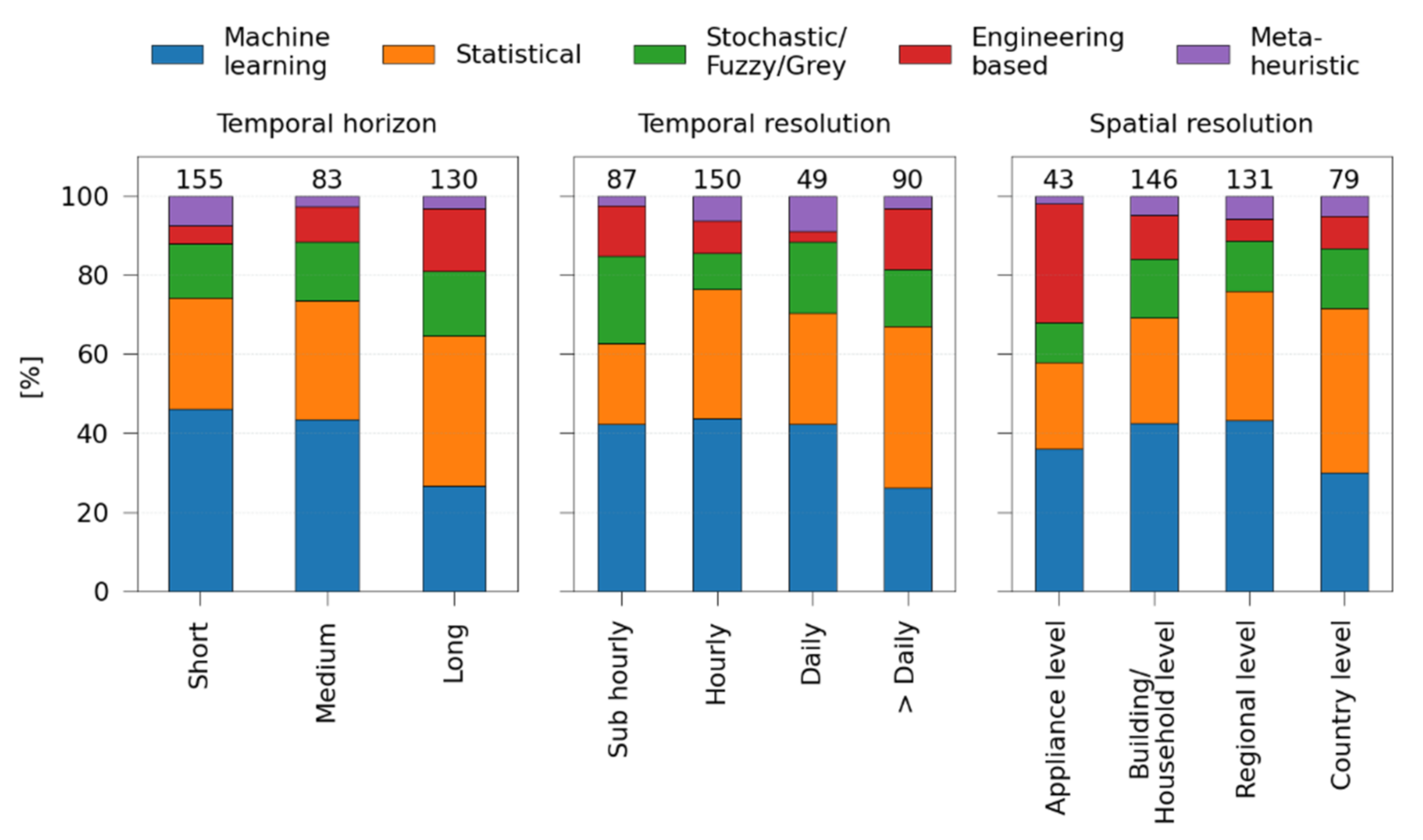
The spatial and temporal properties represent the level of detail applied within the articles and are common decision criteria for model selection since the level of detail of available input data substantially influences the resolution and scale of the output of a model. Figure 8 summarizes the core findings with regard to the applied techniques among the analyzed articles.

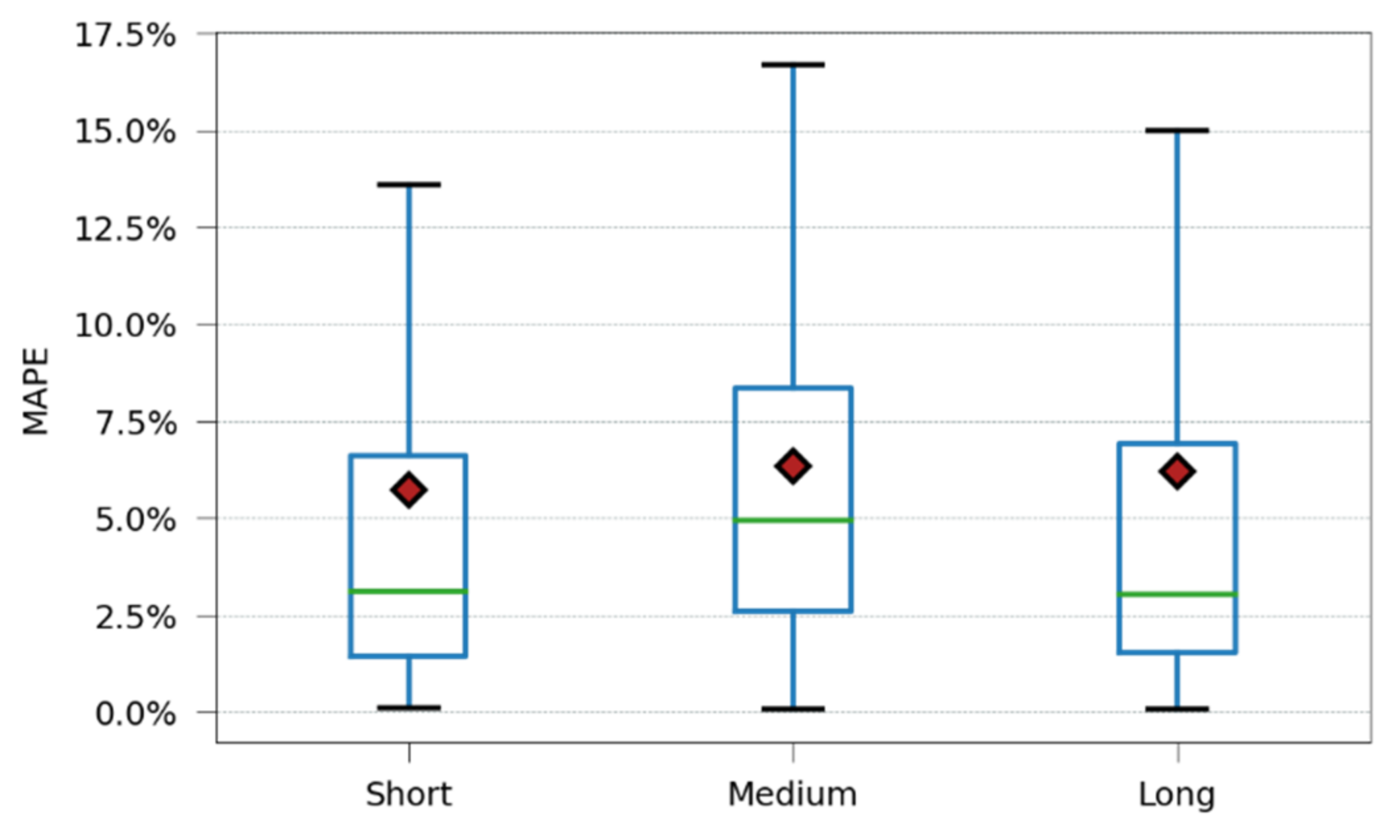
The analysis of the temporal horizon (Figure 8, left) reveals an overall higher number of occurrences for short- (≤one day) and long-term (≥one year) projections compared to medium-term. Among the articles, ML techniques are applied more frequently for short temporal horizons while engineering-based and uncertainty techniques are used more often for longer time frames. This is in line with a common view within the scientific literature, whereby engineering-based energy demand models are described as simulation approaches, which are suitable for modeling longer time spans in a realistic and reliable manner [76]. For the other approaches, there seems to be no particular tendency.

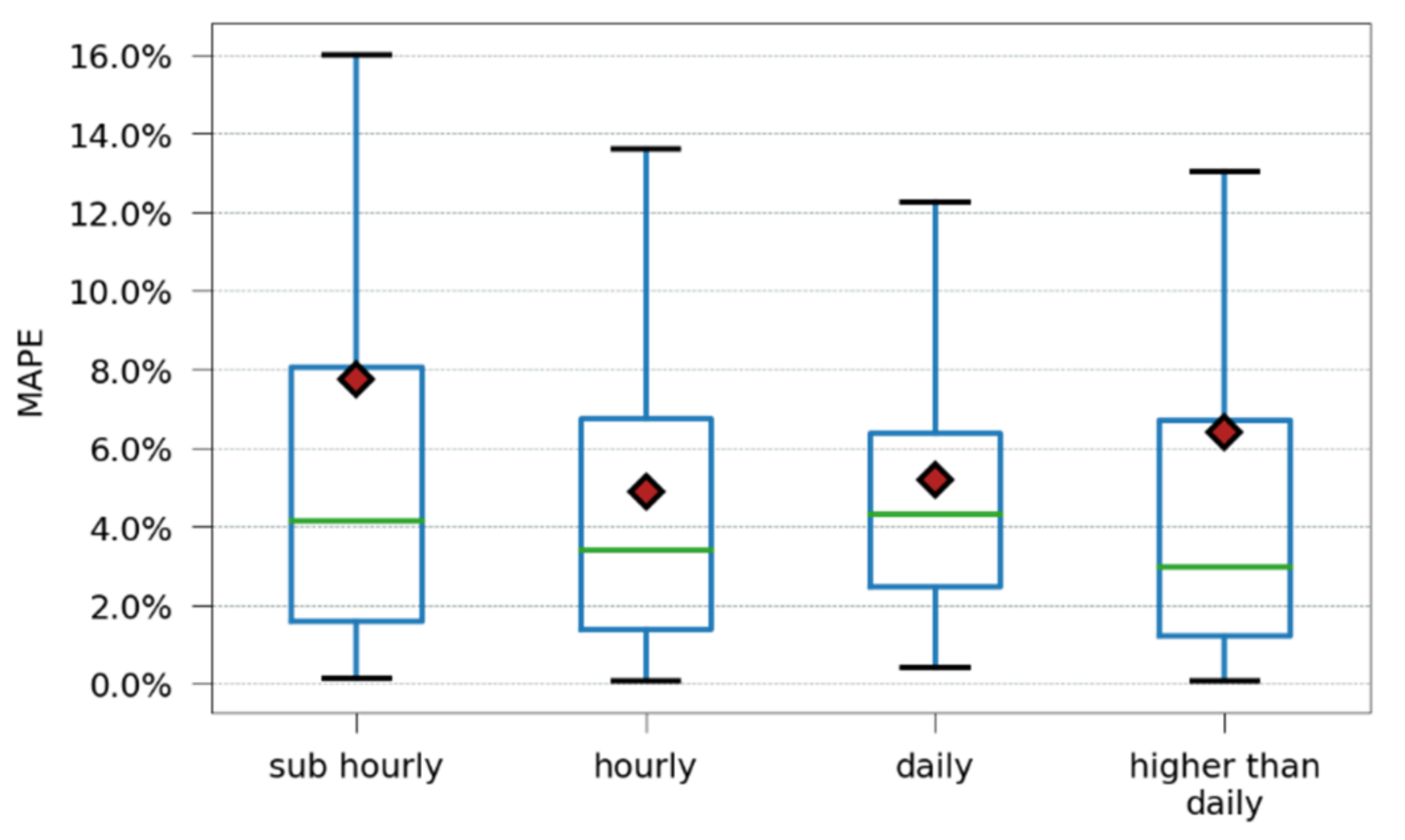
The analysis of the temporal resolution (Figure 8, middle) reveals an overall tendency towards hourly time steps or shorter. This could be because hourly time steps represent a reasonable compromise between the level of detail, availability, and data quantity for most projects since an hourly resolution allows to represent most human-driven impacts on consumption, such as daily routines, while the amount of data is still manageable. Additionally, a lot of weather and consumption data is tracked at least in hourly time steps. However, there are differences among the energy carriers: for example, there was no article that modeled natural gas consumption with shorter than hourly time steps. The difference in temporal resolution for electricity and gas most likely reflects system operation requirements and the respective metering infrastructure [125]. Figure 8 also shows that for time steps longer than one day, there is a decrease of ML approaches while statistical approaches are used more frequently.

The investigation on the spatial resolution (Figure 8, right) shows an overall tendency among the analyzed literature of modeling energy consumption on the level of single households and buildings or regional level, e.g., on a district-scale. Comparatively few approaches focus on the level of appliances or national consumption. Engineering-based techniques stand out in having a clear tendency towards the building and appliance level, reflecting the high level of detail which is characteristic of this technique. Scaling an engineering-based model to the national level requires high amounts of detailed technical system data and has only been done in a few cases [126]. In contrast, statistical techniques are used most frequently on large geographic scales, reflecting their traditional role in econometric analyses.

Table A8. Techniques and level of detail per article (1/2). Compiled results of the analysis on techniques, temporal horizon, and spatial resolution. The table follows a matrix structure: all articles referenced within a cell rely on the category of techniques specified.

Method	Temporal Horizon	Spatial Resolution	References
Machine learning	Short	Appliance	[45,107,163,164,166,236,265]
		Building/household	[40,59,87,91,92,98,112,117,120,130,137,154,162,168,173,175,248,279,323,331,342,346,348,355,360,365,366,369,381,387,392,396,398,399,402,403,407,413,419,448,462,477,478]
		Regional	[37,58,60,71,94,97,106,113,116,135,136,140,146,147,161,165,169,174,176,183,229,235,237,244,249,267,275,286,307,315,319,320,356,434,442,452,459,484]
		National	[16,73,118,155,294,311,317,318,428,432]
	Medium	Appliance	[352,373,474]
		Building/household	[101,102,115,132,143,325,340,349,378,388,395,410,421,445,446,454,456,470,476]
		Regional	[33,68,69,80,90,100,110,111,153,171,260,268,278,288,322,411,449]
		National	[95,191,250,261,263]
	Long	Appliance	n/a
		Building/household	[89,114,156,159,310,328,353,354,380]
		Regional	[21,34,48,70,82,96,103,108,131,141,170,234,270,302,305,309,362,384]
		National	[29,49,51,99,138,178,232,255,258,277,283,285,300,306,312,316,436]
Statistical	Short	Appliance	[231,265,344,418,423]
		Building/household	[59,61,62,63,91,120,154,158,162,168,331,335,335,339,342,346,367,369,379,387,393,394,398,403,407]
		Regional	[30,60,79,113,136,140,146,157,183,227,249,264,276,282,290,356,438,440,442]
		National	[118,142,155,182,242,243,292,294,308,318,330]
	Medium	Appliance	[373,401,420]
		Building/household	[17,75,102,143,180,324,337,338,340,343,390,395,446,473]
		Regional	[247,253,259,268,272,288,289,397,479]
		National	[95,245,246,250,251,261,263,444]
	Long	Appliance	[329]
		Building/household	[85,156,159,160,321,327,333,364,382,404,414]
		Regional	[47,48,96,104,105,131,141,149,150,177,234,241,256,270,271,280,281,296,297,301,305,357,391,397]
		National	[29,83,84,133,134,138,178,179,181,189,192,230,240,255,262,273,277,283,285,298,303,312,313,314,351,371,435,436,439,443]

and

Table A9. Techniques and level of detail per article (2/2). Continuation of Table A6.

Method	Temporal Horizon	Spatial Resolution	References
Stochastic/ Fuzzy/ Grey	Short	Appliance	[45,163,164,418]
		Building/household	[20,40,46,52,59,66,98,112,335,392,393]
		Regional	[30,79,113,135,176,276,299,434]
		National	[16,118,243,257,294,317]
	Medium	Appliance	n/a
		Building/household	[64,75,324,349,385,470]
		Regional	[33,68,69,272,411]
		National	[246,251]
	Long	Appliance	n/a
		Building/household	[114,321,327,347,382,414,463]
		Regional	[34,47,48,70,270,321,334,336,362]
		National	[18,29,49,51,121,133,192,284,285,435]
Meta- heuristic	Short	Appliance	[163]
		Building/household	[40,112,117,175,387,407,413,437]
		Regional	[37,71,116,136,320]
		National	[73]
	Medium	Appliance	n/a
		Building/household	[446]
		Regional	[254]
		National	[191]
	Long	Appliance	n/a
		Building/household	n/a
		Regional	[34,150]
		National	[49,189,190,192]
Engineering-based	Short	Appliance	[274,406,415,467,482]
		Building/household	[52,186,332,461]
		Regional	n/a
		National	[330]
	Medium	Appliance	[474,480]
		Building/household	[19,74,75,78,188,466]
		Regional	[129]
		National	[368]
	Long	Appliance	[194,329,375,483]
		Building/household	[54,77,85,341,347,353,463,481]
		Regional	[187,226,233,287,291,295,334,374,441]
		National	[126]

in Appendix A provide a structured list of references by techniques and levels of detail. The tables allow the reader to identify recent articles that share a similar combination of these properties, which enables fellow researchers to quickly find matching articles for their projects.

4.4. Prediction Accuracy

Prediction accuracy has a direct relationship with decision quality [113]. Therefore, the pursuit of performance enhancement and higher levels of accuracy is one of the driving factors of the development of new techniques and combinations among them. Given its importance, researchers might consider the forecasting accuracy as a criterion for model selection. According to Hong and Fan, the most used performance measure in the electric power industry is MAPE, due to its simplicity and transparency [5]. Lewis’ benchmark [127], which has been mentioned by several authors [18,128], suggests, that a MAPE value of 10 % or lower indicates high prediction accuracy.

In several literature reviews MAPE values of different techniques are compared [4,14,23]. Debnath and Mourshed suggest, that ML and hybrid approaches tend to perform more accurate compared to other techniques [4] and Wei et al. found that MAPE values of long-term projections tend to be better than for short-term projections [14]. However, other authors are reluctant to give clear recommendations, stating that the different choices of performance measures make it hard to categorize the methods from best to worst [4] and that the suitability of models finally depend on the dataset [23].

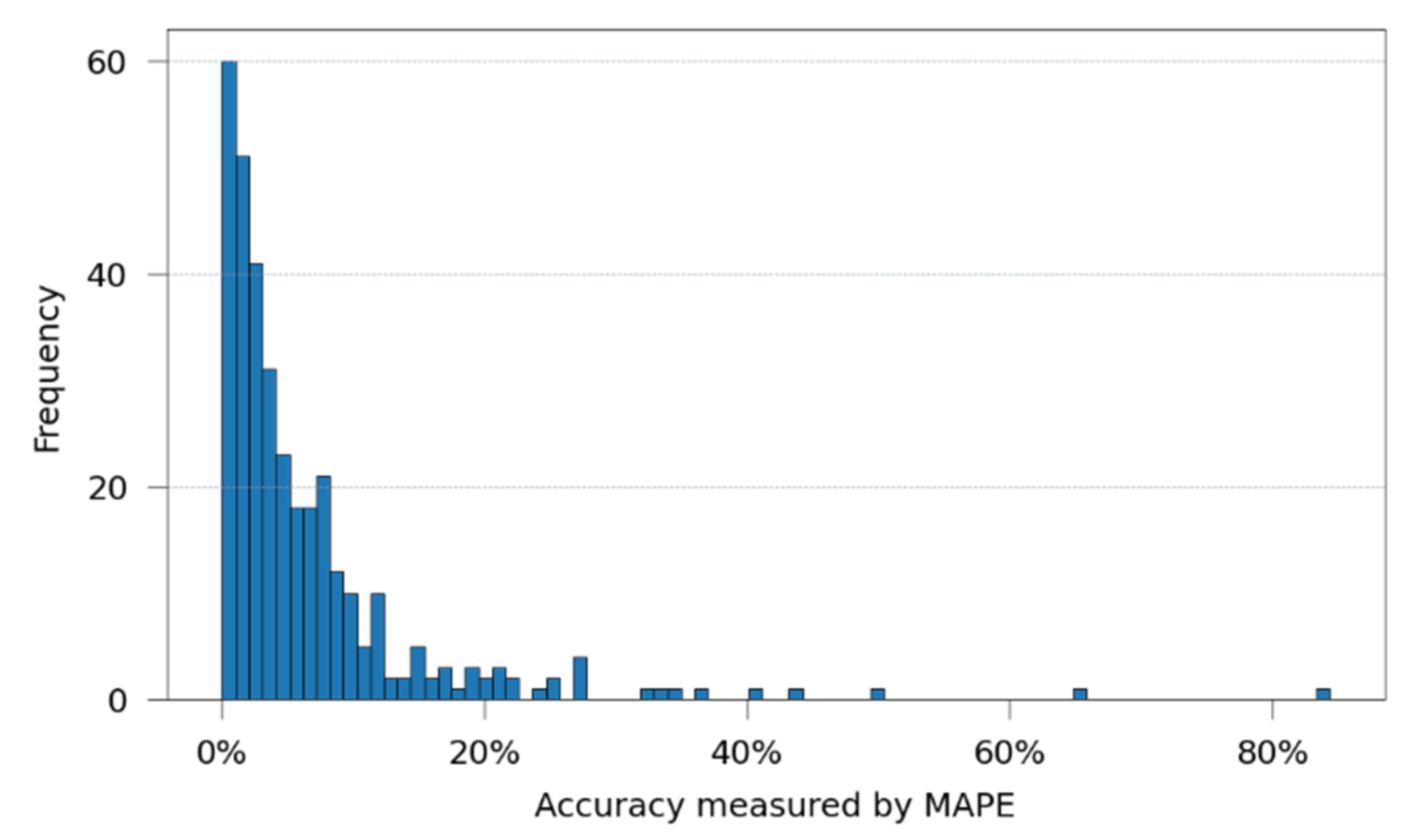
MAPE was the most frequently used accuracy measure among articles and was provided in 217 of 419 articles. Other measures like root mean square error (RMSE), normalized RMSE (nRMSE), mean absolute error (MAE), and coefficient of determination (R²) were encountered in several cases as well. Figure 9 shows the histogram of the MAPE values over-collected from all articles. The shape of the distribution as well as the values for skew (3.99) and kurtosis (23.07) give a strong indication that the values are not normally distributed. The same assumption can be derived from the histograms of the grouped MAPE values, e.g., by technique since they show similar characteristics.

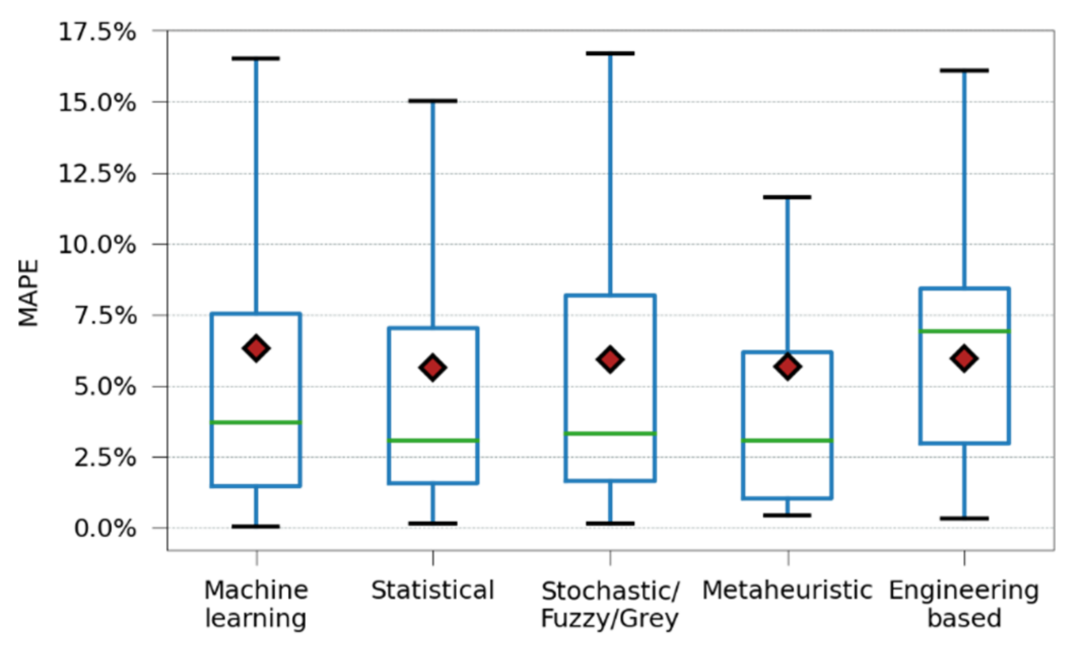
Figure 10 shows that a direct comparison does not reveal a universal higher level of accuracy for any technique used among the articles. While engineering-based methods have a slightly higher median (green line), the means (red diamonds) are almost equal among all techniques. This could be due to the great variety of available methods within each category, allowing users to find techniques that are tailored to their use-cases. Furthermore, for every technique, particular measures and sub-routines have been developed to counter drawbacks and increase accuracy (see Section 4.5). An analysis of the MAPE values of techniques grouped by hybrid and stand-alone approaches yielded a similar result.

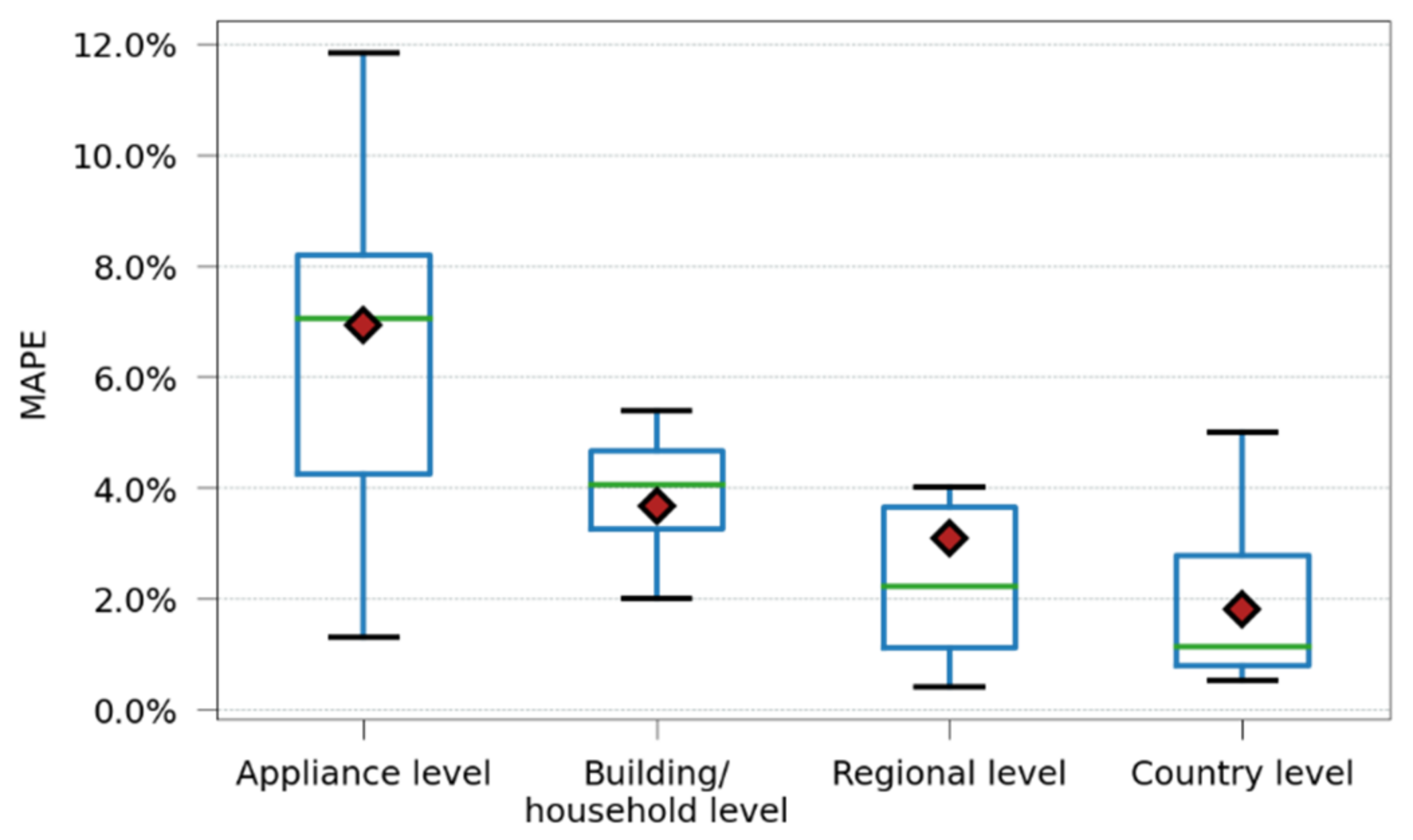
Figure 11 gives an indication, that different levels of spatial resolution could influence the accuracy of prediction. A higher level of detail seems to result in higher MAPE values, especially for articles in which loads of individual appliances were predicted showed. A possible interpretation could be, that aggregated loads on the level of countries or regions are easier to predict since they are smoother and more likely to show seasonal or trend-related patterns compared to loads of individual appliances. Disaggregated loads depend on the behavior of individual users having a higher degree of randomness, which naturally produces lower degrees of accuracy in their prediction. Similar analyses for articles grouped by the temporal horizon and the temporal resolution were conducted but did not show interpretable results (see Figure A1 and Figure A2 in the Appendix A).

4.5. Measures for Improvement of Accuracy

Techniques have become more flexible over the years to be adapted to the specific contexts and datasets in which they are used and sub-routines have been developed to counter drawbacks and improve predictive performance.

For ML techniques, the following measures to improve predictive performance have been found in the analyzed articles. To reduce overfitting, ensemble learning was employed to create independent predictions of multiple models and to use weighted averaged results [59,95,96,97,99,113,115,129,130,131,132,133,134]. Other measures against overfitting include the usage of incremental learning and dynamic neural networks, where the models are updated step by step during training phase [88,106,131,135] or restrictions on coefficients are implemented [136] as well as the introduction of dropout layers [137]. The adjustments of coefficients of the predicting variables in order to capture the essential properties of the training data and provide better generalization to yet unknown data points, is an important and widespread concept to avoid overfitting known as regularization. The idea is to use a regression technique to shrink or regularize the estimated coefficients, effectively discouraging the learning of a complex model and hence reducing risk of overfitting. The most common procedures are the least absolute shrinkage and selection operator (LASSO) [138,139,140,141,142] and the ridge regression [96,102,143,144]. Bayesian regularization was used in [145,146].

The curse of dimensionality [147] is a common problem, which occurs when dealing with high dimensional datasets. Elimination of insignificant features and appropriate selection is crucial for ML and regression techniques. This was achieved by using correlation and principal component analysis (PCA) in [61,107,148,149,150,151,152,153,154,155,156,157,158,159,160,161]. For ML approaches, feature selection was also done by genetic algorithms and decision trees in [39,40,100,111] and fuzzy based feature selection in [162,163,164]. To boost accuracy, deep learning techniques such as stacked auto encoders [21,165,166,167] or long short-term memory (LSTM) networks [153,168,169,170,171] are used. Another measure to increase accuracy for ANN is to vary the number of neurons and layers, as shown in [106,159,172,173].

Another popular measure is the pre-processing of data in order to eliminate outliers and noise, as well as isolate seasonal [113] or temperature related [174] patterns. For TSA and ML techniques this has been done by using wavelet or Fourier transformation in [39,58,90,108,111,120,175,176,177,178,179,180]. Particular attention was payed to the prediction of special events and holidays in [118,181,182,183].

Sometimes model performance suffers from the lack of data. In the case of ML approaches this can be compensated by the creation of virtual data through densification or latent information functions [184,185]. In engineering-based techniques insufficient data can be tackled by prioritization as well as the right choice of representative samples as done in [19,54,186,187,188].

ML approaches sometimes suffer from ending up in local shallow minima when optimizing parameters. The solutions can involve alternative (metaheuristic) optimization routines during training stage, such as the artificial bee colony algorithm for ANNs [116,189], the Cuckoo search [71] or the wolf pack algorithm [163] for SVMs.

4.6. Summary of Results

The following chapter provides a brief summary of advantages and disadvantages as well as countermeasures to cope with the drawbacks by category of techniques derived from the analyzed literature.

Table 9. Summary of advantages and disadvantages as well as countermeasures to compensate drawbacks.

Technique	Advantages	Disadvantages	Countermeasures
ML	High predictive performance; Relatively low implementation effort; Able to handle nonlinear relations; Many pre-set model configurations are available; Can be used without deeper knowledge of technical system	Black box character; Risk of overfitting; Course of dimensionality; Risk of getting stuck in shallow local minima	Regularization; Ensemble learning; Appropriate feature selection; Variation of input layers and neurons; Usage of metaheuristic optimization during the training stage
Statistical	Low implementation effort for basic models; White box character, revealing relations between independent and dependent variables; Especially TSA can be used with relatively low data requirements	Limitations when independent variables are correlated; Difficulties predicting extreme events and outliers; Slight risk of overfitting	Pre-processing of data, e.g., by transformation and decomposition; Variable selection using PCA; Coefficient adjustments using regularization
Stochastic/Fuzzy/Grey	Appropriately addresses uncertainty about inputs allowing to estimate expected outputs and output variations by using quantiles, intervals, or density functions as representations; Able to deal with incomplete/inaccurate data; Able to simulate energy demand based on stochastic processes, providing generated data as inputs for other models	Can be considered unsatisfying for decision-makers since model outputs are afflicted with probabilistic or fuzzy expressions; Long computing times for repeated simulation of stochastic processes	Variable elimination algorithms; Usage of evaluative labels on model outputs to make the uncertainty more understandable (e.g., uncertainty is high or low)
Metaheuristic	Provide alternative and promising methods to solve optimization problems and efficiently search the solution space to find global optima; can be applied to different types of problems; a high number of easy to implement algorithms in place; Can be incorporated into other models;	Requires additional knowledge and effort to implement in existing models; not unrestrictedly reliable in finding the optimal solution Can have low convergence rates and be time-consuming	Usage of existing and proven model combinations
Engineering-based	White-box character, revealing detailed input-output relations based on laws of physics; Able to simulate energy demand for explorative and normative scenarios including disruptions that have no historic record	Data and knowledge-intensive for a description of the technical system; prediction accuracy can be low due to simplifications regarding the system	Prioritization of datasets and choice of representative samples; Use of publicly available datasets for aggregated consumers

contains the most important elements.

ML techniques are used the most across the articles and showed an increase in usage over the last years. ML has the advantages of being able to handle nonlinear relations and achieve high levels of accuracy with quite low implementation effort [22]. Drawbacks lie in the black-box character [190], the tendency of overfitting and getting stuck at shallow local minima [116,191]. Countermeasures are the use of regularization procedures, the formation of model ensembles as well as feature selection and data pre-processing by decomposition. ML techniques dominate across all temporal and spatial levels, however with a slight tendency towards smaller time steps, horizons and scales.

Statistical modelling techniques have a long history in econometrics and are common in energy demand modelling, too. They are the second most used technique. Multiple linear regression is fast and simple to use and capable of explaining the relationship between independent and dependent variables. However, when independent variables are correlated, these models face difficulties [148]. One way of counteracting is by refining the variable selection process and reducing complexity with the help of PCA or coefficient shrinking with LASSO. TSA techniques are easy to use and efficient in modelling overall trends and seasonal patterns. Limits occur when it comes to forecasting extreme events or outliers. Countermeasures can be found in the transformation and decomposition of data [104].

Techniques for stochastic, fuzzy and grey systems modelling address different types of uncertainty. As discussed by Hong and Fan [5], having elements of uncertainty included in model outputs can be considered to be unsatisfying for decision makers in management positions who expect single point values. However, this branch of energy demand modelling can still be considered as a recent development, which will likely see an increase in popularity over the next years. Fuzzy and grey approaches are able to deal with incomplete or inaccurate data [69,192]. Stochastic simulations might run into long computing times, which can be countered by variable elimination algorithms [98].

Meta-heuristic approaches are mainly used as part of combined models, e.g., by introducing genetic feature selection algorithms [40,112] or by optimizing model parameters through an evolutionary process [72,73,189]. However, the integration of a metaheuristic algorithm into another technique requires additional effort and can have low convergence rates that has to be justified by improved results [193].

Engineering-based techniques derive energy demand from a bottom-up representation, which involves a detailed representation of input-output-relationships based on the laws of physics. This level of detail represents a fundamental difference to other techniques. Engineering-based approaches are commonly used in the context of building simulation [57,194]. However, the requirement of large amounts of parameters as well as the accurate representation of input-output relationships make the initial set-up of such models rather laborious. Once created, however, these models have the potential to predict different scenarios on a long temporal horizon, which makes them particularly relevant in the context of system planning. Furthermore, the forecasting based on historic data, as done by ML and TSA techniques, is unable to depict structural disruptions, such as the consequences of political interventions, technological breakthroughs or a pandemic.

5. Discussion

Compared to existing literature reviews on energy demand modelling presented in Section 1 ([4,9,10,11,12,13,14]) and Table A1, this study covers all sectors, energy carriers, categories of techniques, input data types, spatio-temporal characteristics, accuracy as well as advantages, disadvantages and typical countermeasures. A recent publication in this journal by Mosavi et al. [195] focuses on the application of ML models in the energy system comprising separate analyses of multiple studies including accuracy values on different scales. In comparison, the study at hand presents a more detailed analysis of the demand sector, including a wider range of techniques and a more extensive and structured literature base, ensuring comparability of the properties of different articles.

Most articles focus on electricity consumption, which is not surprising since it is the most valuable and expensive form of energy. Moreover, due to service level requirements of grid infrastructure and expansion of smart meters, vast amounts of detailed and high-quality data is available in this sector [5]. However, the authors expect an increasing number of smart metering devices also in the gas and heat grids, which will improve data availability in the future and facilitate integrated energy system planning and modelling [196,197].

Studies with a focus on buildings represent a significant overall share among analyzed articles and are particularly relevant in the context of modelling heating and cooling demand in the residential and commercial sector. Compared to relevant analyses on the building sector assessing efficiency of wood-based constructions [198], their energy consumption during use [199] or the potential of zero energy buildings [200,201], the review at hand covers all energy demand sectors up to a national scale.

The industry sector is underrepresented in the available articles. Considering the intense efforts regarding efficiency targets and demand side management potentials, there is a large interest in modelling the industry sector including the adoption of new technologies, as explained by Fleiter et al. [76]. The small number of articles can be explained by a lack of publicly available data as well as the reluctance to publish this kind of research; energy consumption of a company is often considered sensitive data since it implicitly contains information about production activity and efficiency [125]. The results of the review at hand indicate that the challenges pointed out by Fleiter et al. regarding data availability and transparency in the industrial sector persist [76].

Accuracy of prediction is one of the most important factors in decision making, not only to enable the right choice of models but also to allow stakeholders to understand the performance of the employed method. Unlike the findings of other authors ([4,14]), a tendency of higher accuracy for ML and hybrid techniques or for longer temporal horizons cannot be confirmed for the analyzed articles. It was shown that among the examined literature models with higher spatial detail have a tendency towards lower accuracy. This shows that comparing MAPE values of techniques irrespective of the individual context in which they are applied is of limited explanatory value. In order to robustly compare and discuss accuracy of different techniques they have to be applied to the same datasets, as done in forecasting competitions, such as GEFCom [27,139,202,203,204].

6. Challenges and Future Research Directions

In the context of the energy transition, the focus of planning and decision-making processes is expanding across infrastructures and sectors. Accordingly, the level of detail and complexity of energy systems and energy demand models is increasing. Looking at the results of the analysis, the research focus is on sector-unspecific electricity demand, i.e., without a focus on a particular consumer group. Given the importance of carbon-free energy carriers, a continuous high output of articles on electricity demand is expected but should be backed up by intensifying research on modeling heat and hydrogen demand. Compared to the residential and commercial sectors, the industrial sector has been less frequent in the focus. Given the significant decarbonization challenges this sector faces, intense research efforts are needed and should lead to an increasing number of publicly available studies.

ML-techniques, more precisely ANN, and statistical approaches are the predominant methods and historic energy demand, weather data, and calendar information are the most frequently applied inputs. Based on the analysis of data-technique combinations (Table 4, Table 5, Table 6, Table 7 and Table 8), continuous intensive use of data-driven ML-techniques can be expected, especially in ensembles and combined models integrating key strengths of other models such as Fuzzy expressions or metaheuristic optimization algorithms, using historic energy demand and publicly available input data. At the same time, given the high explanatory value of the technical system and appliance usage data, the authors see a high potential for an intensifying application of these inputs. This development is supported by the expansion of the sensor and metering sector, which will further increase the availability and quality of data, especially on the level of buildings and appliances. In addition, this level of detail is needed in order to accurately model demand flexibility options and their technical and economic constraints in the different sectors. This also enables a broader application of detailed engineering-based models, which are particularly suited for representing the input-output relations.

Future work should make use of the knowledge base provided by this literature review, inspiring hypothesis-driven analyses and quantitative testing, focusing on the applicability and dominance of specific data-method combinations for energy demand modeling.

7. Conclusions

A comprehensive and up-to-date systematic literature review about energy demand modeling regarding techniques, data, accuracy, energy carriers, sectors, and spatio-temporal level of detail was presented. 419 articles published between 2015 and 2020 were reviewed. References are structured by property and compiled in tables for easy access.

The analysis has shown that energy demand modeling is a research field with continuously high numbers of yearly publications. The analysis of the articles proved the current trend of increasing popularity for ML approaches. Statistical models such as regression and TSA are well established, whereas stochastic/fuzzy/grey and metaheuristic techniques often are used as part of combined approaches. Engineering-based techniques stand out as they provide a more detailed representation of the physical properties of the energy-consuming system resulting in higher external and internal data requirements. A research gap was identified regarding models for industrial energy demand.

The level of accuracy proves to be a difficult criterion for a ranking of techniques since attainable performance depends on the particular context. Among the articles, a higher level of detail, e.g., forecasting on the level of appliances, produced lower levels of accuracy compared to forecasts of aggregated loads on country levels.

The material presented here shows trends with regard to the prevailing combinations of methods and data and allows these trends to be tested on the basis of quantitative methods in the future. In particular, this review provides the basis for further analyses and quantitative testing of hypotheses regarding the applicability and dominance of specific methods for sub-categories of demand modeling.

References

- Bai, L.; Li, F.; Cui, H.; Jiang, T.; Sun, H.; Zhu, J. Interval Optimization Based Operating Strategy for Gas-Electricity Integrated Energy Syst. Considering Demand Response and Wind Uncertainty. Appl. Energy 2016, 167, 270–279. [Google Scholar] [CrossRef] [Green Version]
- Lopion, P.; Markewitz, P.; Robinius, M.; Stolten, D. A Review of Current Challenges and Trends in Energy Syst. Modeling. Renew. Sustain. Energy Rev. 2018, 96, 156–166. [Google Scholar] [CrossRef]
- Birol, F. The Investment Implications of Global Energy Trends. Oxf. Rev. Econ. Policy 2005, 21, 145–153. [Google Scholar] [CrossRef]
- Debnath, K.B.; Mourshed, M. Forecasting Methods in Energy Planning Models. Renew. Sustain. Energy Rev. 2018, 88, 297–325. [Google Scholar] [CrossRef] [Green Version]
- Hong, T.; Fan, S. Probabilistic Electric Load Forecasting: A Tutorial Review. Int. J. Forecast. 2016, 32, 914–938. [Google Scholar] [CrossRef]
- Bhattacharyya, S.C.; Timilsina, G.R. Energy Demand Models For Policy Formulation: A Comparative Study Of Energy Demand Models; Policy Research Working Papers; The World Bank: Washington, DC, USA, 2009. [Google Scholar]
- Durach, C.F. A Theoretical and Practical Contribution to Supply Chain Robustness: Developing a Schema for Robustness in Dyads; Straube, F., Baumgartner, H., Klinker, R., Eds.; Schriftenreihe Logistik der Technischen Universität Berlin; Universitätsverlag TU Berlin: Berlin, Germany, 2016; Volume 33, ISBN 978-3-7983-2813-6. [Google Scholar]
- Tranfield, D.; Denyer, D.; Smart, P. Towards a Methodology for Developing Evidence-Informed Management Knowledge by Means of Systematic Review. Br. J. Manag. 2003, 14, 207–222. [Google Scholar] [CrossRef]
- Kuster, C.; Rezgui, Y.; Mourshed, M. Electrical Load Forecasting Models: A Critical Systematic Review. Sustain. Cities Soc. 2017, 35, 257–270. [Google Scholar] [CrossRef]
- Amasyali, K.; El-Gohary, N.M. A Review of Data-Driven Building Energy Consumption Prediction Studies. Renew. Sustain. Energy Rev. 2018, 81, 1192–1205. [Google Scholar] [CrossRef]
- Frederiks, E.; Stenner, K.; Hobman, E.; Frederiks, E.R.; Stenner, K.; Hobman, E.V. The Socio-Demographic and Psychological Predictors of Residential Energy Consumption: A Comprehensive Review. Energies 2015, 8, 573–609. [Google Scholar] [CrossRef] [Green Version]
- Riva, F.; Tognollo, A.; Gardumi, F.; Colombo, E. Long-Term Energy Planning and Demand Forecast in Remote Areas of Developing Countries: Classification of Case Studies and Insights from a Modelling Perspective. Energy Strategy Rev. 2018, 20, 71–89. [Google Scholar] [CrossRef] [Green Version]
- Šebalj, D.; Mesarić, J.; Dujak, D. Analysis of Methods and Techniques for Prediction of Natural Gas Consumption: A Literature Review. J. Inf. Organ. Sci. 2019, 43, 99–117. [Google Scholar] [CrossRef]
- Wei, N.; Li, C.; Peng, X.; Zeng, F.; Lu, X. Conventional Models and Artificial Intelligence-Based Models for Energy Consumption Forecasting: A Review. J. Pet. Sci. Eng. 2019, 181, 106187. [Google Scholar] [CrossRef]
- Matthews, T. LibGuides: Web of Science Platform: Web of Science: Summary of Coverage. Available online: https://clarivate.libguides.com/webofscienceplatform/coverage (accessed on 3 September 2019).
- Shieh, H.-L.; Chen, F.-H. Forecasting for Ultra-Short-Term Electric Power Load Based on Integrated Artificial Neural Networks. Symmetry 2019, 11, 1063. [Google Scholar] [CrossRef] [Green Version]
- Syah, I.F.; Abdullah, M.P.; Syadli, H.; Hassan, M.Y.; Hussin, F. Data Selection Test Method for Better Prediction Of Building Electricity Consumption. J. Teknol. 2016, 78, 67–72. [Google Scholar] [CrossRef]
- Ma, X.; Liu, Z. Application of a Novel Time-Delayed Polynomial Grey Model to Predict the Natural Gas Consumption in China. J. Comput. Appl. Math. 2017, 324, 17–24. [Google Scholar] [CrossRef]
- Chuan, L.; Ukil, A. Modeling and Validation of Electrical Load Profiling in Residential Buildings in Singapore. IEEE Trans. Power Syst. 2015, 30, 2800–2809. [Google Scholar] [CrossRef] [Green Version]
- Sancho-Tomás, A.; Sumner, M.; Robinson, D. A Generalised Model of Electrical Energy Demand from Small Household Appliances. Energy Build. 2017, 135, 350–366. [Google Scholar] [CrossRef]
- Ye, C.; Ding, Y.; Wang, P.; Lin, Z. A Data-Driven Bottom-Up Approach for Spatial and Temporal Electric Load Forecasting. IEEE Trans. Power Syst. 2019, 34, 1966–1979. [Google Scholar] [CrossRef]
- Tien Bui, D.; Moayedi, H.; Anastasios, D.; Kok Foong, L. Predicting Heating and Cooling Loads in Energy-Efficient Buildings Using Two Hybrid Intelligent Models. Appl. Sci. 2019, 9, 3543. [Google Scholar] [CrossRef] [Green Version]
- Fallah, S.; Deo, R.; Shojafar, M.; Conti, M.; Shamshirband, S. Computational Intelligence Approaches for Energy Load Forecasting in Smart Energy Management Grids: State of the Art, Future Challenges, and Research Directions. Energies 2018, 11, 596. [Google Scholar] [CrossRef] [Green Version]
- Motulsky, H.J.; Ransnas, L.A. Fitting Curves to Data Using Nonlinear Regression: A Practical and Nonmathematical Review. FASEB J. 1987, 1, 365–374. [Google Scholar] [CrossRef]
- Huang, Y.; Yuan, Y.; Chen, H.; Wang, J.; Guo, Y.; Ahmad, T. A Novel Energy Demand Prediction Strategy for Residential Buildings Based on Ensemble Learning. Energy Procedia 2019, 158, 3411–3416. [Google Scholar] [CrossRef]
- Charytoniuk, W.; Chen, M.S.; Van Olinda, P. Nonparametric Regression Based Short-Term Load Forecasting. IEEE Trans. Power Syst. 1998, 13, 725–730. [Google Scholar] [CrossRef]
- Mangalova, E.; Shesterneva, O. Sequence of Nonparametric Models for GEFCom2014 Probabilistic Electric Load Forecasting. Int. J. Forecast. 2016, 32, 1023–1028. [Google Scholar] [CrossRef]
- Ghalehkhondabi, I.; Ardjmand, E.; Weckman, G.R.; Young, W.A. An Overview of Energy Demand Forecasting Methods Published in 2005–2015. Energy Syst. 2017, 8, 411–447. [Google Scholar] [CrossRef]
- Kavaklioglu, K. Principal Components Based Robust Vector Autoregression Prediction of Turkey’s Electricity Consumption. Energy Syst. 2019, 10, 889–910. [Google Scholar] [CrossRef]
- Nagbe, K.; Cugliari, J.; Jacques, J. Short-Term Electricity Demand Forecasting Using a Functional State Space Model. Energies 2018, 11, 1120. [Google Scholar] [CrossRef] [Green Version]
- Russell, S.J.; Norvig, P. Artificial Intelligence: A Modern Approach; Prentice Hall series in artificial intelligence; Prentice Hall: Englewood Cliffs, NJ, USA, 1995; ISBN 978-0-13-103805-9. [Google Scholar]
- Singh, A.; Thakur, N.; Sharma, A. A Review of Supervised Machine Learning Algorithms. In Proceedings of the 2016 3rd International Conference on Computing for Sustainable Global Development, New Delhi, India, 16–18 March 2016; pp. 1310–1315. [Google Scholar]
- Alamaniotis, M.; Bargiotas, D.; Tsoukalas, L.H. Towards Smart Energy Syst.: Application of Kernel Machine Regression for Medium Term Electricity Load Forecasting. SpringerPlus 2016, 5, 58. [Google Scholar] [CrossRef] [Green Version]
- Song, Z.; Niu, D.; Dai, S.; Xiao, X.; Wang, Y. Incorporating the Influence of China’s Industrial Capacity Elimination Policies in Electricity Demand Forecasting. Util. Policy 2017, 47, 1–11. [Google Scholar] [CrossRef]
- Brownlee, J. Master Machine Learning Algorithms—Discover How They Work and Implement Them From Scratch; Machine Learning Mastery: Vermont, VIC, Australia, 2016. [Google Scholar]
- Tzanetos, A.; Dounias, G. An Application-Based Taxonomy of Nature Inspired Intelligent Algorithms; MDE Lab: Chios, Greece, 2019. [Google Scholar]
- Al-Shammari, E.T.; Keivani, A.; Shamshirband, S.; Mostafaeipour, A.; Yee, P.L.; Petković, D.; Ch, S. Prediction of Heat Load in District Heating Systems by Support Vector Machine with Firefly Searching Algorithm. Energy 2016, 95, 266–273. [Google Scholar] [CrossRef]
- Nur, A.S.; Mohd Radzi, N.H.; Ibrahim, A.O. Artificial Neural Network Weight Optimization: A Review. Telkomnika Indones. J. Electr. Eng. 2014, 12, 6897–6902. [Google Scholar] [CrossRef]
- Saleh, A.I.; Rabie, A.H.; Abo-Al-Ez, K.M. A Data Mining Based Load Forecasting Strategy for Smart Electrical Grids. Adv. Eng. Inform. 2016, 30, 422–448. [Google Scholar] [CrossRef]
- Eseye, A.T.; Lehtonen, M.; Tukia, T.; Uimonen, S.; John Millar, R. Machine Learning Based Integrated Feature Selection Approach for Improved Electricity Demand Forecasting in Decentralized Energy Syst. IEEE Access 2019, 7, 91463–91475. [Google Scholar] [CrossRef]
- Zimmermann, H.-J. Fuzzy Set Theory—And Its Applications; Springer Netherlands: Dordrecht, 2001; ISBN 978-94-010-3870-6. [Google Scholar]
- Hájek, P.; Godo, L.; Esteva, F. Fuzzy Logic and Probability. arXiv 2013, arXiv:1302.4953. [Google Scholar]
- Riedewald, F. Comparison of Deterministic, Stochastic and Fuzzy Logic Uncertainty Modelling for Capacity Extension Projects of DI/WFI Pharmaceutical Plant Utilities with Variable/Dynamic Demand. Ph.D. Thesis, University College Cork, Cork, Ireland, 2011. [Google Scholar]
- Ferrández-Pastor, F.J.; Mora-Mora, H.; Sánchez-Romero, J.L.; Nieto-Hidalgo, M.; García-Chamizo, J.M. Interpreting Human Activity from Electrical Consumption Data Using Reconfigurable Hardware and Hidden Markov Models. J. Ambient Intell. Human. Comput. 2017, 8, 469–483. [Google Scholar] [CrossRef]
- Andersson, M. Modeling Electricity Load Curves with Hidden Markov Models for Demand-Side Management Status Estimation: Modeling Electricity Load Curves. Int. Trans. Electr. Energy Syst. 2017, 27, e2265. [Google Scholar] [CrossRef]
- Duan, Q.; Liu, J.; Zhao, D. A Fast Algorithm for Short Term Electric Load Forecasting by a Hidden Semi-Markov Process. J. Stat. Comput. Simul. 2019, 89, 831–843. [Google Scholar] [CrossRef]
- Ismail, Z.; Efendi, R.; Deris, M.M. Application of Fuzzy Time Series Approach in Electric Load Forecasting. New Math. Nat. Comput. 2015, 11, 229–248. [Google Scholar] [CrossRef]
- Laouafi, A.; Mordjaoui, M.; Laouafi, F.; Boukelia, T.E. Daily Peak Electricity Demand Forecasting Based on an Adaptive Hybrid Two-Stage Methodology. Int. J. Electr. Power Energy Syst. 2016, 77, 136–144. [Google Scholar] [CrossRef]
- Mollaiy-Berneti, S. Optimal Design of Adaptive Neuro-Fuzzy Inference System Using Genetic Algorithm for Electricity Demand Forecasting in Iranian Industry. Soft Comput. 2016, 20, 4897–4906. [Google Scholar] [CrossRef]
- Tien, T.-L. A New Grey Prediction Model FGM(1, 1). Soft Comput. 2009, 49, 1416–1426. [Google Scholar] [CrossRef]
- Hu, Y.-C. Electricity Consumption Prediction Using a Neural-Network-Based Grey Forecasting Approach. J. Oper. Res. Soc. 2017, 68, 1259–1264. [Google Scholar] [CrossRef]
- McKenna, E.; Thomson, M. High-Resolution Stochastic Integrated Thermal–Electrical Domestic Demand Model. Appl. Energy 2016, 165, 445–461. [Google Scholar] [CrossRef] [Green Version]
- Rehfeldt, M.; Fleiter, T.; Toro, F. A Bottom-up Estimation of the Heating and Cooling Demand in European Industry. Energy Effic. 2018, 11, 1057–1082. [Google Scholar] [CrossRef]
- Nouvel, R.; Zirak, M.; Coors, V.; Eicker, U. The Influence of Data Quality on Urban Heating Demand Modeling Using 3D City Models. Comput. Environ. Urban Syst. 2017, 64, 68–80. [Google Scholar] [CrossRef]
- Li, C. GIS for Urban Energy Analysis. In Comprehensive Geographic Information Systems; Elsevier: Amsterdam, The Netherlands, 2018; pp. 187–195. ISBN 978-0-12-804793-4. [Google Scholar]
- Prerna, R.; Gangopadhyay, P.K. Demand Forecasting of Electricity and Optimal Locationing of Transformer Locations Using Geo-Spatial Techniques: A Case Study of Districts of Bihar, India. Appl. Spat. Anal. Policy 2015, 8, 69–83. [Google Scholar] [CrossRef]
- D’Alonzo, V.; Novelli, A.; Vaccaro, R.; Vettorato, D.; Albatici, R.; Diamantini, C.; Zambelli, P. A Bottom-up Spatially Explicit Methodology to Estimate the Space Heating Demand of the Building Stock at Regional Scale. Energy Build. 2020, 206, 109581. [Google Scholar] [CrossRef]
- Ivanov, V.V.; Kryanev, A.V.; Osetrov, E.S. Forecasting the Daily Electricity Consumption in the Moscow Region Using Artificial Neural Networks. Phys. Part. Nuclei Lett. 2017, 14, 647–657. [Google Scholar] [CrossRef]
- Laouafi, A.; Mordjaoui, M.; Haddad, S.; Boukelia, T.E.; Ganouche, A. Online Electricity Demand Forecasting Based on an Effective Forecast Combination Methodology. Electr. Power Syst. Res. 2017, 148, 35–47. [Google Scholar] [CrossRef]
- Ren, Y.; Suganthan, P.N.; Srikanth, N.; Amaratunga, G. Random Vector Functional Link Network for Short-Term Electricity Load Demand Forecasting. Inf. Sci. 2016, 367–368, 1078–1093. [Google Scholar] [CrossRef]
- Kipping, A.; Trømborg, E. Modeling Hourly Consumption of Electricity and District Heat in Non-Residential Buildings. Energy 2017, 123, 473–486. [Google Scholar] [CrossRef]
- Morita, K.; Shiromaru, H.; Manabe, Y.; Kato, T.; Funabashi, T.; Suzuoki, Y. A Study on Estimation of Aggregated Electricity Demand for One-Hour-Ahead Forecast. Appl. Therm. Eng. 2017, 114, 1443–1448. [Google Scholar] [CrossRef]
- Sandels, C.; Widén, J.; Nordström, L.; Andersson, E. Day-Ahead Predictions of Electricity Consumption in a Swedish Office Building from Weather, Occupancy, and Temporal Data. Energy Build. 2015, 108, 279–290. [Google Scholar] [CrossRef]
- Shepero, M.; van der Meer, D.; Munkhammar, J.; Widén, J. Residential Probabilistic Load Forecasting: A Method Using Gaussian Process Designed for Electric Load Data. Appl. Energy 2018, 218, 159–172. [Google Scholar] [CrossRef]
- Ziegler, F.; Seim, S.; Verwiebe, P.; Müller-Kirchenbauer, J. A Probabilistic Modelling Approach for Residential Load Profiles. Energ. Ressour. 2020, 1–28. [Google Scholar] [CrossRef]
- Ge, Y.; Zhou, C.; Hepburn, D.M. Domestic Electricity Load Modelling by Multiple Gaussian Functions. Energy Build. 2016, 126, 455–462. [Google Scholar] [CrossRef] [Green Version]
- Verdejo, H.; Awerkin, A.; Becker, C.; Olguin, G. Statistic Linear Parametric Techniques for Residential Electric Energy Demand Forecasting. A Review and an Implementation to Chile. Renew. Sustain. Energy Rev. 2017, 74, 512–521. [Google Scholar] [CrossRef]
- Dong, B.; Li, Z.; Rahman, S.M.M.; Vega, R. A Hybrid Model Approach for Forecasting Future Residential Electricity Consumption. Energy Build. 2016, 117, 341–351. [Google Scholar] [CrossRef]
- Lou, C.W.; Dong, M.C. A Novel Random Fuzzy Neural Networks for Tackling Uncertainties of Electric Load Forecasting. Int. J. Electr. Power Energy Syst. 2015, 73, 34–44. [Google Scholar] [CrossRef]
- Ali, D.; Yohanna, M.; Ijasini, P.M.; Garkida, M.B. Application of Fuzzy – Neuro to Model Weather Parameter Variability Impacts on Electrical Load Based on Long-Term Forecasting. Alex. Eng. J. 2018, 57, 223–233. [Google Scholar] [CrossRef]
- Zhang, X.; Wang, J.; Zhang, K. Short-Term Electric Load Forecasting Based on Singular Spectrum Analysis and Support Vector Machine Optimized by Cuckoo Search Algorithm. Electr. Power Syst. Res. 2017, 146, 270–285. [Google Scholar] [CrossRef]
- Khan, G.M.; Zafari, F. Dynamic Feedback Neuro-Evolutionary Networks for Forecasting the Highly Fluctuating Electrical Loads. Genet. Program. Evolvable Mach. 2016, 17, 391–408. [Google Scholar] [CrossRef]
- Khan, G.M.; Arshad, R. Electricity Peak Load Forecasting Using CGP Based Neuro Evolutionary Techniques. Int. J. Comput. Intell. Syst. 2016, 9, 376–395. [Google Scholar] [CrossRef] [Green Version]
- Perera, D.; Skeie, N.-O. Comparison of Space Heating Energy Consumption of Residential Buildings Based on Traditional and Model-Based Techniques. Buildings 2017, 7, 27. [Google Scholar] [CrossRef] [Green Version]
- Muthalib, M.K.; Nwankpa, C.O. Physically-Based Building Load Model for Electric Grid Operation and Planning. IEEE Trans. Smart Grid 2017, 8, 169–177. [Google Scholar] [CrossRef]
- Fleiter, T.; Worrell, E.; Eichhammer, W. Barriers to Energy Effic in Industrial Bottom-up Energy Demand Models—A Review. Renew. Sustain. Energy Rev. 2011, 15, 3099–3111. [Google Scholar] [CrossRef]
- Cao, J.; Liu, J.; Man, X. A United WRF/TRNSYS Method for Estimating the Heating/Cooling Load for the Thousand-Meter Scale Megatall Buildings. Appl. Therm. Eng. 2017, 114, 196–210. [Google Scholar] [CrossRef]
- Nam, T.H.H.; Kubota, T.; Trihamdani, A.R. Impact of Urban Heat Island under the Hanoi Master Plan 2030 on Cooling Loads in Residential Buildings. Int. J. Built Environ. Sustain. 2015, 2, 48–61. [Google Scholar] [CrossRef]
- Lopez, J.C.; Rider, M.J.; Wu, Q. Parsimonious Short-Term Load Forecasting for Optimal Operation Planning of Electrical Distribution Systems. IEEE Trans. Power Syst. 2019, 34, 1427–1437. [Google Scholar] [CrossRef] [Green Version]
- Xue, G.; Song, J.; Kong, X.; Pan, Y.; Qi, C.; Li, H. Prediction of Natural Gas Consumption for City-Level DHS Based on Attention GRU: A Case Study for a Northern Chinese City. IEEE Access 2019, 7, 130685–130699. [Google Scholar] [CrossRef]
- Salvó, G.; Piacquadio, M.N. Multifractal Analysis of Electricity Demand as a Tool for Spatial Forecasting. Energy Sustain. Dev. 2017, 38, 67–76. [Google Scholar] [CrossRef]
- Zhao, T.; Zhang, Y.; Chen, H. Spatio-Temporal Load Forecasting Considering Aggregation Features of Electricity Cells and Uncertainties in Input Variables. J. Electr. Eng. Technol. 2018, 13, 38–50. [Google Scholar]
- Brabec, M.; Konár, O.; Kasanický, I.; Malý, M.; Pelikán, E. Semiparametric Modeling of the Spatiotemporal Trends in Natural Gas Consumption: Methodology, Results, and Consequences. Appl. Stoch. Models Bus. Ind. 2020, 36, 184–194. [Google Scholar] [CrossRef] [Green Version]
- Falchetta, G.; Noussan, M. Interannual Variation in Night-Time Light Radiance Predicts Changes in National Electricity Consumption Conditional on Income-Level and Region. Energies 2019, 12, 456. [Google Scholar] [CrossRef] [Green Version]
- Bednar, D.J.; Reames, T.G.; Keoleian, G.A. The Intersection of Energy and Justice: Modeling the Spatial, Racial/Ethnic and Socioeconomic Patterns of Urban Residential Heating Consumption and Efficiency in Detroit, Michigan. Energy Build. 2017, 143, 25–34. [Google Scholar] [CrossRef]
- Deng, C.; Lin, W.; Ye, X.; Li, Z.; Zhang, Z.; Xu, G. Social Media Data as a Proxy for Hourly Fine-Scale Electric Power Consumption Estimation. Environ. Plan. A Econ. Space 2018, 50, 1553–1557. [Google Scholar] [CrossRef] [Green Version]
- Wang, H.; Tu, F.; Tu, B.; Feng, G.; Yuan, G.; Ren, H.; Dong, J. Neural Network Based Central Heating System Load Prediction and Constrained Control. Math. Probl. Eng. 2018, 2018, 2908608. [Google Scholar] [CrossRef] [Green Version]
- Mordjaoui, M.; Haddad, S.; Medoued, A.; Laouafi, A. Electric Load Forecasting by Using Dynamic Neural Network. Int. J. Hydrog. Energy 2017, 42, 17655–17663. [Google Scholar] [CrossRef]
- Duan, J.; Qiu, X.; Ma, W.; Tian, X.; Shang, D. Electricity Consumption Forecasting Scheme via Improved LSSVM with Maximum Correntropy Criterion. Entropy 2018, 20, 112. [Google Scholar] [CrossRef] [PubMed] [Green Version]
- Fan, G.-F.; Peng, L.-L.; Hong, W.-C.; Sun, F. Electric Load Forecasting by the SVR Model with Differential Empirical Mode Decomposition and Auto Regression. Neurocomputing 2016, 173, 958–970. [Google Scholar] [CrossRef]
- Wang, J.; Li, G.; Chen, H.; Liu, J.; Guo, Y.; Sun, S.; Hu, Y. Energy Consumption Prediction for Water-Source Heat Pump System Using Pattern Recognition-Based Algorithms. Appl. Therm. Eng. 2018, 136, 755–766. [Google Scholar] [CrossRef]
- Li, Y.; Guo, P.; Li, X. Short-Term Load Forecasting Based on the Analysis of User Electricity Behavior. Algorithms 2016, 9, 80. [Google Scholar] [CrossRef] [Green Version]
- Melzi, F.N.; Same, A.; Zayani, M.H.; Oukhellou, L. A Dedicated Mixture Model for Clustering Smart Meter Data: Identification and Analysis of Electricity Consumption Behaviors. Energies 2017, 10, 1446. [Google Scholar] [CrossRef] [Green Version]
- Huang, N.; Lu, G.; Xu, D. A Permutation Importance-Based Feature Selection Method for Short-Term Electricity Load Forecasting Using Random Forest. Energies 2016, 9, 767. [Google Scholar] [CrossRef] [Green Version]
- De Oliveira, E.M.; Cyrino Oliveira, F.L. Forecasting Mid-Long Term Electric Energy Consumption through Bagging ARIMA and Exponential Smoothing Methods. Energy 2018, 144, 776–788. [Google Scholar] [CrossRef]
- Chen, K.; Jiang, J.; Zheng, F.; Chen, K. A Novel Data-Driven Approach for Residential Electricity Consumption Prediction Based on Ensemble Learning. Energy 2018, 150, 49–60. [Google Scholar] [CrossRef]
- Khwaja, A.S.; Zhang, X.; Anpalagan, A.; Venkatesh, B. Boosted Neural Networks for Improved Short-Term Electric Load Forecasting. Electr. Power Syst. Res. 2017, 143, 431–437. [Google Scholar] [CrossRef]
- Bassamzadeh, N.; Ghanem, R. Multiscale Stochastic Prediction of Electricity Demand in Smart Grids Using Bayesian Networks. Appl. Energy 2017, 193, 369–380. [Google Scholar] [CrossRef]
- Zhang, W.; Yang, J. Forecasting Natural Gas Consumption in China by Bayesian Model Averaging. Energy Rep. 2015, 1, 216–220. [Google Scholar] [CrossRef] [Green Version]
- Huang, N.; Hu, Z.; Cai, G.; Yang, D. Short Term Electrical Load Forecasting Using Mutual Information Based Feature Selection with Generalized Minimum-Redundancy and Maximum-Relevance Criteria. Entropy 2016, 18, 330. [Google Scholar] [CrossRef] [Green Version]
- Idowu, S.; Saguna, S.; Åhlund, C.; Schelén, O. Applied Machine Learning: Forecasting Heat Load in District Heating System. Energy Build. 2016, 133, 478–488. [Google Scholar] [CrossRef]
- Cao, L.; Li, Y.; Zhang, J.; Jiang, Y.; Han, Y.; Wei, J. Electrical Load Prediction of Healthcare Buildings through Single and Ensemble Learning. Energy Rep. 2020, 6, 2751–2767. [Google Scholar] [CrossRef]
- Leme, J.V.; Casaca, W.; Colnago, M.; Dias, M.A. Towards Assessing the Electricity Demand in Brazil: Data-Driven Analysis and Ensemble Learning Models. Energies 2020, 13, 1407. [Google Scholar] [CrossRef] [Green Version]
- Akpinar, M.; Yumusak, N. Year Ahead Demand Forecast of City Natural Gas Using Seasonal Time Series Methods. Energies 2016, 9, 727. [Google Scholar] [CrossRef]
- Boroojeni, K.G.; Amini, M.H.; Bahrami, S.; Iyengar, S.S.; Sarwat, A.I.; Karabasoglu, O. A Novel Multi-Time-Scale Modeling for Electric Power Demand Forecasting: From Short-Term to Medium-Term Horizon. Electr. Power Syst. Res. 2017, 142, 58–73. [Google Scholar] [CrossRef]
- Qiu, X.; Suganthan, P.N.; Amaratunga, G.A.J. Ensemble Incremental Learning Random Vector Functional Link Network for Short-Term Electric Load Forecasting. Knowl. Based Syst. 2018, 145, 182–196. [Google Scholar] [CrossRef]
- Ding, Y.; Zhang, Q.; Yuan, T.; Yang, K. Model Input Selection for Building Heating Load Prediction: A Case Study for an Office Building in Tianjin. Energy Build. 2018, 159, 254–270. [Google Scholar] [CrossRef]
- Weide, L.; Demeng, K.; Jinran, W. A Novel Hybrid Model Based on Extreme Learning Machine, k-Nearest Neighbor Regression and Wavelet Denoising Applied to Short-Term Electric Load Forecasting. Energies 2017, 10, 694. [Google Scholar] [CrossRef] [Green Version]
- Koo, B.-G.; Lee, H.-S.; Park, J. Short-Term Electric Load Forecasting Based on Wavelet Transform and GMDH. J. Electr. Eng. Technol. 2015, 10, 832–837. [Google Scholar] [CrossRef] [Green Version]
- Rana, M.; Koprinska, I. Forecasting Electricity Load with Advanced Wavelet Neural Networks. Neurocomputing 2016, 182, 118–132. [Google Scholar] [CrossRef]
- Yaslan, Y.; Bican, B. Empirical Mode Decomposition Based Denoising Method with Support Vector Regression for Time Series Prediction: A Case Study for Electricity Load Forecasting. Measurement 2017, 103, 52–61. [Google Scholar] [CrossRef]
- Panapakidis, I.P.; Dagoumas, A.S. Day-Ahead Natural Gas Demand Forecasting Based on the Combination of Wavelet Transform and ANFIS/Genetic Algorithm/Neural Network Model. Energy 2017, 118, 231–245. [Google Scholar] [CrossRef]
- Chahkoutahi, F.; Khashei, M. A Seasonal Direct Optimal Hybrid Model of Computational Intelligence and Soft Comput. Techniques for Electricity Load Forecasting. Energy 2017, 140, 988–1004. [Google Scholar] [CrossRef]
- Jovanovic, R.; Sretenovic, A. Various Multistage Ensembles for Prediction of Heating Energy Consumption. Modeling Identif. Control. A Nor. Res. Bull. 2015, 36, 119–132. [Google Scholar] [CrossRef] [Green Version]
- Jovanovic, R.; Sretenovic, A.; Zivkovic, B. Multistage Ensemble of Feedforward Neural Networks for Prediction of Heating Energy Consumption. Therm. Sci. 2016, 20, 1321–1331. [Google Scholar] [CrossRef] [Green Version]
- Akpinar, M.; Adak, M.; Yumusak, N. Day-Ahead Natural Gas Demand Forecasting Using Optimized ABC-Based Neural Network with Sliding Window Technique: The Case Study of Regional Basis in Turkey. Energies 2017, 10, 781. [Google Scholar] [CrossRef] [Green Version]
- Bianchi, F.M.; Santis, E.D.; Rizzi, A.; Sadeghian, A. Short-Term Electric Load Forecasting Using Echo State Networks and PCA Decomposition. IEEE Access 2015, 3, 1931–1943. [Google Scholar] [CrossRef]
- Brodowski, S.; Bielecki, A.; Filocha, M. A Hybrid System for Forecasting 24-h Power Load Profile for Polish Electric Grid. Appl. Soft Comput. 2017, 58, 527–539. [Google Scholar] [CrossRef]
- Pang, Y.; Yao, B.; Zhou, X.; Zhang, Y.; Xu, Y.; Tan, Z. Hierarchical Electricity Time Series Forecasting for Integrating Consumption Patterns Analysis and Aggregation Consistency. In Proceedings of the Twenty-Seventh International Joint Conference on Artificial Intelligence, Stockholm, Sweden, 13–19 July 2018; International Joint Conferences on Artificial Intelligence Organization: Stockholm, Sweden; pp. 3506–3512.
- Li, C.; Zheng, X.; Yang, Z.; Kuang, L. Predicting Short-Term Electricity Demand by Combining the Advantages of ARMA and XGBoost in Fog Computing Environment. Wirel. Commun. Mob. Comput. 2018, 2018, 5018053. [Google Scholar] [CrossRef]
- Fischer, D.; Härtl, A.; Wille-Haussmann, B. Model for Electric Load Profiles with High Time Resolution for German Households. Energy Build. 2015, 92, 170–179. [Google Scholar] [CrossRef]
- Marszal-Pomianowska, A.; Heiselberg, P.; Kalyanova Larsen, O. Household Electricity Demand Profiles – A High-Resolution Load Model to Facilitate Modelling of Energy Flexible Buildings. Energy 2016, 103, 487–501. [Google Scholar] [CrossRef]
- Xu, M.; Singh, S. China Liberalises Coal-Fired Power Pricing to Tackle Energy Crisis; Reuters: London, UK, 2021; Volume 1, p. 1. [Google Scholar]
- Labandeira, X.; Labeaga, J.M.; López-Otero, X. A Meta-Analysis on the Price Elasticity of Energy Demand. Energy Policy 2017, 102, 549–568. [Google Scholar] [CrossRef] [Green Version]
- Seim, S.; Verwiebe, P.; Blech, K.; Gerwin, C.; Müller-Kirchenbauer, J. Die Datenlandschaft der deutschen Energiewirtschaft; Zenodo: Meyrin, Switzerland, 2019. [Google Scholar] [CrossRef]
- Maçaira, P.; Elsland, R.; Oliveira, F.C.; Souza, R.; Fernandes, G. Forecasting Residential Electricity Consumption: A Bottom-up Approach for Brazil by Region. Energy Effic. 2020, 13, 911–934. [Google Scholar] [CrossRef]
- Lewis, C.D. Industrial and Business Forecasting Methods: A Practical Guide to Exponential Smoothing and Curve Fitting; Butterworth S Scientific: London, UK; Boston, MA, USA, 1982; ISBN 978-0-408-00559-3. [Google Scholar]
- Wei, Y.; Zhang, X.; Shi, Y.; Xia, L.; Pan, S.; Wu, J.; Han, M.; Zhao, X. A Review of Data-Driven Approaches for Prediction and Classification of Building Energy Consumption. Renew. Sustain. Energy Rev. 2018, 82, 1027–1047. [Google Scholar] [CrossRef]
- Hu, Z.; Ma, J.; Yang, L.; Li, X.; Pang, M. Decomposition-Based Dynamic Adaptive Combination Forecasting for Monthly Electricity Demand. Sustainability 2019, 11, 1272. [Google Scholar] [CrossRef] [Green Version]
- Lee, J.; Kim, J.; Ko, W. Day-Ahead Electric Load Forecasting for the Residential Building with a Small-Size Dataset Based on a Self-Organizing Map and a Stacking Ensemble Learning Method. Appl. Sci. 2019, 9, 1231. [Google Scholar] [CrossRef] [Green Version]
- Grmanová, G.; Laurinec, P.; Rozinajová, V.; Ezzeddine, A.B.; Lucká, M.; Lacko, P.; Vrablecová, P.; Návrat, P. Incremental Ensemble Learning for Electricity Load Forecasting. Acta Polytech. Hung. 2016, 13, 97–117. [Google Scholar] [CrossRef]
- Shan, S.; Cao, B.; Wu, Z. Forecasting the Short-Term Electricity Consumption of Building Using a Novel Ensemble Model. IEEE Access 2019, 7, 88093–88106. [Google Scholar] [CrossRef]
- Zhang, X.; Zhou, W. Forecast of China’s Natural Gas Consumption Using Mathematical Models. Energy Sources Part B Econ. Plan. Policy 2018, 13, 246–250. [Google Scholar] [CrossRef]
- Liang, J.; Liang, Y. Analysis and Modeling for China’s Electricity Demand Forecasting Based on a New Mathematical Hybrid Method. Information 2017, 8, 33. [Google Scholar] [CrossRef] [Green Version]
- Lu, X.; Wang, J.; Cai, Y.; Zhao, J. Distributed HS-ARTMAP and Its Forecasting Model for Electricity Load. Appl. Soft Comput. 2015, 32, 13–22. [Google Scholar] [CrossRef]
- Buitrago, J.; Asfour, S. Short-Term Forecasting of Electric Loads Using Nonlinear Autoregressive Artificial Neural Networks with Exogenous Vector Inputs. Energies 2017, 10, 40. [Google Scholar] [CrossRef] [Green Version]
- Zhu, R.; Guo, W.; Gong, X. Short-Term Load Forecasting for CCHP Systems Considering the Correlation between Heating, Gas and Electrical Loads Based on Deep Learning. Energies 2019, 12, 3308. [Google Scholar] [CrossRef] [Green Version]
- Sigauke, C. Forecasting Medium-Term Electricity Demand in a South African Electric Power Supply System. J. Energy South. Afr. 2017, 28, 54–67. [Google Scholar] [CrossRef]
- Ziel, F.; Liu, B. Lasso Estimation for GEFCom 2014 Probabilistic Electric Load Forecasting. Int. J. Forecast. 2016, 32, 1029–1037. [Google Scholar] [CrossRef] [Green Version]
- Takeda, H.; Tamura, Y.; Sato, S. Using the Ensemble Kalman Filter for Electricity Load Forecasting and Analysis. Energy 2016, 104, 184–198. [Google Scholar] [CrossRef]
- He, Y.; Qin, Y.; Wang, S.; Wang, X.; Wang, C. Electricity Consumption Probability Density Forecasting Method Based on LASSO-Quantile Regression Neural Network. Appl. Energy 2019, 233–234, 565–575. [Google Scholar] [CrossRef] [Green Version]
- Lebotsa, M.E.; Sigauke, C.; Bere, A.; Fildes, R.; Boylan, J.E. Short Term Electricity Demand Forecasting Using Partially Linear Additive Quantile Regression with an Application to the Unit Commitment Problem. Appl. Energy 2018, 222, 104–118. [Google Scholar] [CrossRef] [Green Version]
- Yu, C.; Mirowski, P.; Ho, T.K. A Sparse Coding Approach to Household Electricity Demand Forecasting in Smart Grids. IEEE Trans. Smart Grid 2017, 8, 738–748. [Google Scholar] [CrossRef]
- Srihari, J.; Santhi, B. Prediction of Heating and Cooling Load to Improve Energy Effic. of Buildings Using Machine Learning Techniques. J. Mech. Contin. Math. Sci. 2018, 13, 97–113. [Google Scholar] [CrossRef]
- Kim, M.; Cha, J.; Lee, E.; Pham, V.; Lee, S.; Theera-Umpon, N. Simplified Neural Network Model Design with Sensitivity Analysis and Electricity Consumption Prediction in a Commercial Building. Energies 2019, 12, 1201. [Google Scholar] [CrossRef] [Green Version]
- Potočnik, P.; Strmčnik, E.; Govekar, E. Linear and Neural Network-Based Models for Short-Term Heat Load Forecasting. Stroj. Vestn. J. Mech. Eng. 2015, 61, 543–550. [Google Scholar] [CrossRef]
- Cecati, C.; Kolbusz, J.; Rozycki, P.; Siano, P.; Wilamowski, B.M. A Novel RBF Training Algorithm for Short-Term Electric Load Forecasting and Comparative Studies. IEEE Trans. Ind. Electron. 2015, 62, 6519–6529. [Google Scholar] [CrossRef]
- Ismail, N.; Abdullah, S. Principal Component Regression with Artificial Neural Network to Improve Prediction of Electricity Demand. Int. Arab J. Inf. Technol. 2016, 13, 7. [Google Scholar]
- Vu, D.H.; Muttaqi, K.M.; Agalgaonkar, A.P. A Variance Inflation Factor and Backward Elimination Based Robust Regression Model for Forecasting Monthly Electricity Demand Using Climatic Variables. Appl. Energy 2015, 140, 385–394. [Google Scholar] [CrossRef] [Green Version]
- Amber, K.P.; Aslam, M.W.; Hussain, S.K. Electricity Consumption Forecasting Models for Administration Buildings of the UK Higher Education Sector. Energy Build. 2015, 90, 127–136. [Google Scholar] [CrossRef]
- Chen, H.-Y.; Lee, C.-H. Electricity Consumption Prediction for Buildings Using Multiple Adaptive Network-Based Fuzzy Inference System Models and Gray Relational Analysis. Energy Rep. 2019, 5, 1509–1524. [Google Scholar] [CrossRef]
- Pepplow, L.A.; Betini, R.C.; Pereira, T.C.G. Forecasting the Electricity Consumption in a Higher Education Institution. Braz. Arch. Biol. Technol. 2019, 62, 1–10. [Google Scholar] [CrossRef]
- Wei, N.; Li, C.; Duan, J.; Liu, J.; Zeng, F. Daily Natural Gas Load Forecasting Based on a Hybrid Deep Learning Model. Energies 2019, 12, 218. [Google Scholar] [CrossRef] [Green Version]
- Yuan, T.; Zhu, N.; Shi, Y.; Chang, C.; Yang, K.; Ding, Y. Sample Data Selection Method for Improving the Prediction Accuracy of the Heating Energy Consumption. Energy Build. 2018, 158, 234–243. [Google Scholar] [CrossRef]
- Martínez-Álvarez, F.; Schmutz, A.; Asencio-Cortés, G.; Jacques, J. A Novel Hybrid Algorithm to Forecast Functional Time Series Based on Pattern Sequence Similarity with Application to Electricity Demand. Energies 2018, 12, 94. [Google Scholar] [CrossRef] [Green Version]
- Gordillo-Orquera, R.; Lopez-Ramos, L.; Muñoz-Romero, S.; Iglesias-Casarrubios, P.; Arcos-Avilés, D.; Marques, A.; Rojo-Álvarez, J. Analyzing and Forecasting Electrical Load Consumption in Healthcare Buildings. Energies 2018, 11, 493. [Google Scholar] [CrossRef] [Green Version]
- Afshari, A.; Luiz A., F. Inverse Modeling of the Urban Energy System Using Hourly Electricity Demand and Weather Measurements, Part 1: Black-Box Model. Energy Build. 2017, 157, 126–138. [Google Scholar] [CrossRef]
- Calili, R.F.; Souza, R.C.; Musafir, J.; Mendes Pinho, J.A. Correction of Load Curves Estimated by Electrical Appliances Ownership Surveys Using Mass Memory Meters. Energy Effic. 2018, 11, 261–272. [Google Scholar] [CrossRef]
- Gunay, B.; Shen, W.; Newsham, G. Inverse Blackbox Modeling of the Heating and Cooling Load in Office Buildings. Energy Build. 2017, 142, 200–210. [Google Scholar] [CrossRef] [Green Version]
- Koivisto, M.; Degefa, M.; Ali, M.; Ekström, J.; Millar, J.; Lehtonen, M. Statistical Modeling of Aggregated Electricity Consumption and Distributed Wind Generation in Distribution Systems Using AMR Data. Electr. Power Syst. Res. 2015, 129, 217–226. [Google Scholar] [CrossRef]
- Gao, X.; Li, X.; Zhao, B.; Ji, W.; Jing, X.; He, Y. Short-Term Electricity Load Forecasting Model Based on EMD-GRU with Feature Selection. Energies 2019, 12, 1140. [Google Scholar] [CrossRef] [Green Version]
- Jurado, S.; Nebot, À.; Mugica, F.; Avellana, N. Hybrid Methodologies for Electricity Load Forecasting: Entropy-Based Feature Selection with Machine Learning and Soft Comput. Techniques. Energy 2015, 86, 276–291. [Google Scholar] [CrossRef] [Green Version]
- Zhang, X. Short-Term Load Forecasting for Electric Bus Charging Stations Based on Fuzzy Clustering and Least Squares Support Vector Machine Optimized by Wolf Pack Algorithm. Energies 2018, 11, 1449. [Google Scholar] [CrossRef] [Green Version]
- Rabie, A.H.; Ali, S.H.; Ali, H.A.; Saleh, A.I. A Fog Based Load Forecasting Strategy for Smart Grids Using Big Electrical Data. Clust. Comput. 2019, 22, 241–270. [Google Scholar] [CrossRef]
- Ke, K.; Hongbin, S.; Chengkang, Z.; Brown, C. Short-Term Electrical Load Forecasting Method Based on Stacked Auto-Encoding and GRU Neural Network. Evol. Intell. 2019, 12, 385–394. [Google Scholar] [CrossRef]
- Chen, Q.; Xia, M.; Lu, T.; Jiang, X.; Liu, W.; Sun, Q. Short-Term Load Forecasting Based on Deep Learning for End-User Transformer Subject to Volatile Electric Heating Loads. IEEE Access 2019, 7, 162697–162707. [Google Scholar] [CrossRef]
- Lu, S.; Lin, G.; Que, H.; Chen, L.; Liu, H.; Ye, C.; Yi, D. Electric Load Data Characterising and Forecasting Based on Trend Index and Auto-Encoders. J. Eng. 2018, 2018, 1915–1921. [Google Scholar] [CrossRef]
- Xu, L.; Li, C.; Xie, X.; Zhang, G. Long-Short-Term Memory Network Based Hybrid Model for Short-Term Electrical Load Forecasting. Information 2018, 9, 165. [Google Scholar] [CrossRef] [Green Version]
- Zhang, D.; Tong, H.; Li, F.; Xiang, L.; Ding, X. An Ultra-Short-Term Electrical Load Forecasting Method Based on Temperature-Factor-Weight and LSTM Model. Energies 2020, 13, 4875. [Google Scholar] [CrossRef]
- Shao, X.; Kim, C.-S.; Sontakke, P. Accurate Deep Model for Electricity Consumption Forecasting Using Multi-Channel and Multi-Scale Feature Fusion CNN–LSTM. Energies 2020, 13, 1881. [Google Scholar] [CrossRef] [Green Version]
- Lin, T.; Pan, Y.; Xue, G.; Song, J.; Qi, C. A Novel Hybrid Spatial-Temporal Attention-LSTM Model for Heat Load Prediction. IEEE Access 2020, 8, 159182–159195. [Google Scholar] [CrossRef]
- Abedinia, O.; Amjady, N. Short-Term Load Forecast of Electrical Power System by Radial Basis Function Neural Network and New Stochastic Search Algorithm. Int. Trans. Electr. Energy Syst. 2016, 26, 1511–1525. [Google Scholar] [CrossRef]
- Pîrjan, A.; Oprea, S.-V.; Căruțașu, G.; Petroșanu, D.-M.; Bâra, A.; Coculescu, C.; Pîrjan, A.; Oprea, S.-V.; Căruțașu, G.; Petroșanu, D.-M.; et al. Devising Hourly Forecasting Solutions Regarding Electricity Consumption in the Case of Commercial Center Type Consumers. Energies 2017, 10, 1727. [Google Scholar] [CrossRef] [Green Version]
- Amara, F.; Agbossou, K.; Dubé, Y.; Kelouwani, S.; Cardenas, A.; Bouchard, J. Household Electricity Demand Forecasting Using Adaptive Conditional Density Estimation. Energy Build. 2017, 156, 271–280. [Google Scholar] [CrossRef]
- Protić, M.; Shamshirband, S.; Petković, D.; Abbasi, A.; Mat Kiah, M.L.; Unar, J.A.; Živković, L.; Raos, M. Forecasting of Consumers Heat Load in District Heating Systems Using the Support Vector Machine with a Discrete Wavelet Transform Algorithm. Energy 2015, 87, 343–351. [Google Scholar] [CrossRef]
- Kong, Z.; Xia, Z.; Cui, Y.; Lv, H. Probabilistic Forecasting of Short-Term Electric Load Demand: An Integration Scheme Based on Correlation Analysis and Improved Weighted Extreme Learning Machine. Appl. Sci. 2019, 9, 4215. [Google Scholar] [CrossRef] [Green Version]
- Yukseltan, E.; Yucekaya, A.; Bilge, A.H. Hourly Electricity Demand Forecasting Using Fourier Analysis with Feedback. Energy Strategy Rev. 2020, 31, 100524. [Google Scholar] [CrossRef]
- Guo, H.; Chen, Q.; Xia, Q.; Kang, C.; Zhang, X. A Monthly Electricity Consumption Forecasting Method Based on Vector Error Correction Model and Self-Adaptive Screening Method. Int. J. Electr. Power Energy Syst. 2018, 95, 427–439. [Google Scholar] [CrossRef]
- Brożyna, J.; Mentel, G.; Szetela, B.; Strielkowski, W. Multi-Seasonality in the TBATS Model Using Demand for Electric Energy as a Case Study. Econ. Comput. Econ. Cybern. Stud. Res. 2018, 52, 229–246. [Google Scholar] [CrossRef]
- Lakovic, M.; Pavlovic, I.; Banjac, M.; Jovic, M.; Mancic, M. Numerical Computation and Prediction of Electricity Consumption in Tobacco Industry. Facta Univ. Ser. Mech. Eng. 2017, 15, 457–465. [Google Scholar] [CrossRef] [Green Version]
- Yukseltan, E.; Yucekaya, A.; Bilge, A.H. Forecasting Electricity Demand for Turkey: Modeling Periodic Variations and Demand Segregation. Appl. Energy 2017, 193, 287–296. [Google Scholar] [CrossRef]
- Trull, Ó.; García-Díaz, J.; Troncoso, A. Application of Discrete-Interval Moving Seasonalities to Spanish Electricity Demand Forecasting during Easter. Energies 2019, 12, 1083. [Google Scholar] [CrossRef] [Green Version]
- Dahl, M.; Brun, A.; Kirsebom, O.; Andresen, G. Improving Short-Term Heat Load Forecasts with Calendar and Holiday Data. Energies 2018, 11, 1678. [Google Scholar] [CrossRef] [Green Version]
- Rego, L.; Sumaili, J.; Miranda, V.; Francês, C.; Silva, M.; Santana, Á. Mean Shift Densification of Scarce Data Sets in Short-Term Electric Power Load Forecasting for Special Days. Electr Eng 2017, 99, 881–898. [Google Scholar] [CrossRef]
- Chang, C.-J.; Lin, J.-Y.; Chang, M.-J. Extended Modeling Procedure Based on the Projected Sample for Forecasting Short-Term Electricity Consumption. Adv. Eng. Inform. 2016, 30, 211–217. [Google Scholar] [CrossRef]
- Wedeward, K.; Adkins, C.; Schaffer, S.; Smith, M.; Patel, A. Inventory of Load Models in Electric Power Systems via Parameter Estimation. Eng. Lett. 2015, 23, 9. [Google Scholar]
- Stefanovic, A.; Gordic, D. Modeling Methodology of the Heating Energy Consumption and the Potential Reductions Due to Thermal Improvements of Staggered Block Buildings. Energy Build. 2016, 125, 244–253. [Google Scholar] [CrossRef]
- Yan, C.; Wang, S.; Shan, K.; Lu, Y. A Simplified Analytical Model to Evaluate the Impact of Radiant Heat on Building Cooling Load. Appl. Therm. Eng. 2015, 77, 30–41. [Google Scholar] [CrossRef]
- Wang, J.; Zhang, J.; Nie, J. An Improved Artificial Colony Algorithm Model for Forecasting Chinese Electricity Consumption and Analyzing Effect Mechanism. Math. Probl. Eng. 2016, 2016, 8496971. [Google Scholar] [CrossRef]
- Mousavi, S.M.; Mostafavi, E.S.; Hosseinpour, F. Towards Estimation of Electricity Demand Utilizing a Robust Multi-Gene Genetic Programming Technique. Energy Effic. 2015, 8, 1169–1180. [Google Scholar] [CrossRef]
- Jawad, M.; Ali, S.M.; Khan, B.; Mehmood, C.A.; Farid, U.; Ullah, Z.; Usman, S.; Fayyaz, A.; Jadoon, J.; Tareen, N.; et al. Genetic Algorithm-Based Non-Linear Auto-Regressive with Exogenous Inputs Neural Network Short-Term and Medium-Term Uncertainty Modelling and Prediction for Electrical Load and Wind Speed. J. Eng. 2018, 2018, 721–729. [Google Scholar] [CrossRef]
- Fan, G.-F.; Wang, A.; Hong, W.-C. Combining Grey Model and Self-Adapting Intelligent Grey Model with Genetic Algorithm and Annual Share Changes in Natural Gas Demand Forecasting. Energies 2018, 11, 1625. [Google Scholar] [CrossRef] [Green Version]
- Ezugwu, A.E.; Adeleke, O.J.; Akinyelu, A.A.; Viriri, S. A Conceptual Comparison of Several Metaheuristic Algorithms on Continuous Optimisation Problems. Neural Comput. Applic 2020, 32, 6207–6251. [Google Scholar] [CrossRef]
- Razavi, S.H.; Ahmadi, R.; Zahedi, A. Modeling, Simulation and Dynamic Control of Solar Assisted Ground Source Heat Pump to Provide Heating Load and DHW. Appl. Therm. Eng. 2018, 129, 127–144. [Google Scholar] [CrossRef]
- Mosavi, A.; Salimi, M.; Faizollahzadeh Ardabili, S.; Rabczuk, T.; Shamshirband, S.; Varkonyi-Koczy, A.R. State of the Art of Machine Learning Models in Energy Syst, a Systematic Review. Energies 2019, 12, 1301. [Google Scholar] [CrossRef] [Green Version]
- Montuori, L.; Alcázar-Ortega, M.; Mansó-Borràs, I.; Vargas-Salgado, C. Communication Technologies in Smart Grids of Natural Gas: New Challenges. In Proceedings of the 2020 Global Congress on Electrical Engineering (GC-ElecEng 2020), Valencia, Spain, 4–6 September 2020; pp. 101–105. [Google Scholar]
- Stănişteanu, C. Smart Thermal Grids—A Review. Sci. Bull. Electr. Eng. Fac. 2017, 17, 36. [Google Scholar] [CrossRef] [Green Version]
- Švajlenka, J.; Kozlovská, M. Evaluation of the Efficiency and Sustainability of Timber-Based Construction. J. Clean. Prod. 2020, 259, 120835. [Google Scholar] [CrossRef]
- Švajlenka, J.; Kozlovská, M. Effect of Accumulation Elements on the Energy Consumption of Wood Constructions. Energy Build. 2019, 198, 160–169. [Google Scholar] [CrossRef]
- Belussi, L.; Barozzi, B.; Bellazzi, A.; Danza, L.; Devitofrancesco, A.; Fanciulli, C.; Ghellere, M.; Guazzi, G.; Meroni, I.; Salamone, F.; et al. A Review of Performance of Zero Energy Buildings and Energy Efficiency Solutions. J. Build. Eng. 2019, 25, 100772. [Google Scholar] [CrossRef]
- Danza, L.; Belussi, L.; Salamone, F. A Multiple Linear Regression Approach to Correlate the Indoor Environmental Factors to the Global Comfort in a Zero-Energy Building. E3S Web Conf. 2020, 197, 04002. [Google Scholar] [CrossRef]
- Dordonnat, V.; Pichavant, A.; Pierrot, A. GEFCom2014 Probabilistic Electric Load Forecasting Using Time Series and Semi-Parametric Regression Models. Int. J. Forecast. 2016, 32, 1005–1011. [Google Scholar] [CrossRef]
- Xie, J.; Hong, T. GEFCom2014 Probabilistic Electric Load Forecasting: An Integrated Solution with Forecast Combination and Residual Simulation. Int. J. Forecast. 2016, 32, 1012–1016. [Google Scholar] [CrossRef]
- Hong, T. GEFCom. 2017. Available online: http://www.drhongtao.com/gefcom/2017 (accessed on 5 May 2021).
- Liu, Z.; Wu, D.; Liu, Y.; Han, Z.; Lun, L.; Gao, J.; Jin, G.; Cao, G. Accuracy Analyses and Model Comparison of Machine Learning Adopted in Building Energy Consumption Prediction. Energy Explor. Exploit. 2019, 37, 1426–1451. [Google Scholar] [CrossRef] [Green Version]
- Kumar, K.P.; Saravanan, B. Recent Techniques to Model Uncertainties in Power Generation from Renewable Energy Sources and Loads in Microgrids – A Review. Renew. Sustain. Energy Rev. 2017, 71, 348–358. [Google Scholar] [CrossRef]
- Wan Alwi, S.R.; Klemeš, J.J.; Varbanov, P.S. Cleaner Energy Planning, Management and Technologies: Perspectives of Supply-Demand Side and End-of-Pipe Management. J. Clean. Prod. 2016, 136, 1–13. [Google Scholar] [CrossRef]
- Mat Daut, M.A.; Hassan, M.Y.; Abdullah, H.; Rahman, H.A.; Abdullah, M.P.; Hussin, F. Building Electrical Energy Consumption Forecasting Analysis Using Conventional and Artificial Intelligence Methods: A Review. Renew. Sustain. Energy Rev. 2017, 70, 1108–1118. [Google Scholar] [CrossRef]
- Khuntia, S.R.; Rueda, J.L.; van der Meijden, M.A.M.M. Forecasting the Load of Electrical Power Systems in Mid- and Long-Term Horizons: A Review. IET Gener. Transm. Distrib. 2016, 10, 3971–3977. [Google Scholar] [CrossRef] [Green Version]
- Torriti, J. A Review of Time Use Models of Residential Electricity Demand. Renew. Sustain. Energy Rev. 2014, 37, 265–272. [Google Scholar] [CrossRef]
- Yildiz, B.; Bilbao, J.I.; Sproul, A.B. A Review and Analysis of Regression and Machine Learning Models on Commercial Building Electricity Load Forecasting. Renew. Sustain. Energy Rev. 2017, 73, 1104–1122. [Google Scholar] [CrossRef]
- Zhou, L.; Li, J.; Li, F.; Meng, Q.; Li, J.; Xu, X. Energy Consumption Model and Energy Effic. of Machine Tools: A Comprehensive Literature Review. J. Clean. Prod. 2016, 112, 3721–3734. [Google Scholar] [CrossRef]
- Mahmud, K.; Town, G.E. A Review of Computer Tools for Modeling Electric Vehicle Energy Requirements and Their Impact on Power Distribution Networks. Appl. Energy 2016, 172, 337–359. [Google Scholar] [CrossRef]
- Mavromatidis, L.E. A Review on Hybrid Optimization Algorithms to Coalesce Computational Morphogenesis with Interactive Energy Consumption Forecasting. Energy Build. 2015, 106, 192–202. [Google Scholar] [CrossRef]
- Frayssinet, L.; Merlier, L.; Kuznik, F.; Hubert, J.-L.; Milliez, M.; Roux, J.-J. Modeling the Heating and Cooling Energy Demand of Urban Buildings at City Scale. Renew. Sustain. Energy Rev. 2018, 81, 2318–2327. [Google Scholar] [CrossRef] [Green Version]
- Deb, C.; Zhang, F.; Yang, J.; Lee, S.E.; Shah, K.W. A Review on Time Series Forecasting Techniques for Building Energy Consumption. Renew. Sustain. Energy Rev. 2017, 74, 902–924. [Google Scholar] [CrossRef]
- Pengwei, S.; Xue, T.; Yan, W.; Shuai, D.; Jun, Z.; Qingsong, A.; Yongzhen, W. Recent Trends in Load Forecasting Technology for the Operation Optimization of Distributed Energy System. Energies 2017, 10, 1303. [Google Scholar] [CrossRef] [Green Version]
- Fumo, N.; Rafe Biswas, M.A. Regression Analysis for Prediction of Residential Energy Consumption. Renew. Sustain. Energy Rev. 2015, 47, 332–343. [Google Scholar] [CrossRef]
- Ahmad, A.S.; Hassan, M.Y.; Abdullah, M.P.; Rahman, H.A.; Hussin, F.; Abdullah, H.; Saidur, R. A Review on Applications of ANN and SVM for Building Electrical Energy Consumption Forecasting. Renew. Sustain. Energy Rev. 2014, 33, 102–109. [Google Scholar] [CrossRef]
- Ahmad, T.; Chen, H.; Guo, Y.; Wang, J. A Comprehensive Overview on the Data Driven and Large Scale Based Approaches for Forecasting of Building Energy Demand: A Review. Energy Build. 2018, 165, 301–320. [Google Scholar] [CrossRef]
- Rafique, S.F.; Jianhua, Z. Energy Management System, Generation and Demand Predictors: A Review. IET Gener. Transm. Distrib. 2017, 12, 519–530. [Google Scholar] [CrossRef]
- Shao, Z.; Chao, F.; Yang, S.-L.; Zhou, K.-L. A Review of the Decomposition Methodology for Extracting and Identifying the Fluctuation Characteristics in Electricity Demand Forecasting. Renew. Sustain. Energy Rev. 2017, 75, 123–136. [Google Scholar] [CrossRef]
- Cabeza, L.F.; Palacios, A.; Serrano, S.; Ürge-Vorsatz, D.; Barreneche, C. Comparison of Past Projections of Global and Regional Primary and Final Energy Consumption with Historical Data. Renew. Sustain. Energy Rev. 2018, 82, 681–688. [Google Scholar] [CrossRef] [Green Version]
- Salisu, A.A.; Ayinde, T.O. Modeling Energy Demand: Some Emerging Issues. Renew. Sustain. Energy Rev. 2016, 54, 1470–1480. [Google Scholar] [CrossRef]
- Fiot, J.-B.; Dinuzzo, F. Electricity Demand Forecasting by Multi-Task Learning. IEEE Trans. Smart Grid 2018, 9, 544–551. [Google Scholar] [CrossRef] [Green Version]
- He, Y.; Jiao, J.; Chen, Q.; Ge, S.; Chang, Y.; Xu, Y. Urban Long Term Electricity Demand Forecast Method Based on System Dynamics of the New Economic Normal: The Case of Tianjin. Energy 2017, 133, 9–22. [Google Scholar] [CrossRef]
- Vu, D.H.; Muttaqi, K.M.; Agalgaonkar, A.P.; Bouzerdoum, A. Short-Term Electricity Demand Forecasting Using Autoregressive Based Time Varying Model Incorporating Representative Data Adjustment. Appl. Energy 2017, 205, 790–801. [Google Scholar] [CrossRef]
- Alani, A.Y.; Osunmakinde, I.O.; Alani, A.Y.; Osunmakinde, I.O. Short-Term Multiple Forecasting of Electric Energy Loads for Sustainable Demand Planning in Smart Grids for Smart Homes. Sustainability 2017, 9, 1972. [Google Scholar] [CrossRef] [Green Version]
- Tong, C.; Li, J.; Lang, C.; Kong, F.; Niu, J.; Rodrigues, J.J.P.C. An Efficient Deep Model for Day-Ahead Electricity Load Forecasting with Stacked Denoising Auto-Encoders. J. Parallel Distrib. Comput. 2018, 117, 267–273. [Google Scholar] [CrossRef]
- Mokilane, P.; Galpin, J.; Yadavalli, V.S.S.; Debba, P.; Koen, R.; Sibiya, S. Density Forecasting for Long-Term Electricity Demand in South Africa Using Quantile Regression. South Afr. J. Econ. Manag. Sci. 2018, 21, a1757. [Google Scholar] [CrossRef]
- Bikcora, C.; Verheijen, L.; Weiland, S. Density Forecasting of Daily Electricity Demand with ARMA-GARCH, CAViaR, and CARE Econometric Models. Sustain. Energy Grids Netw. 2018, 13, 148–156. [Google Scholar] [CrossRef]
- Nadimi, R.; Tokimatsu, K. Modeling of Quality of Life in Terms of Energy and Electricity Consumption. Appl. Energy 2018, 212, 1282–1294. [Google Scholar] [CrossRef]
- Yan, Q.; Qin, C.; Nie, M.; Yang, L. Forecasting the Electricity Demand and Market Shares in Retail Electricity Market Based on System Dynamics and Markov Chain. Math. Probl. Eng. 2018, 2018, 4671850. [Google Scholar] [CrossRef]
- Li, J.; Chen, L.; Xiang, Y.; Li, J.; Peng, D. Influencing Factors and Development Trend Analysis of China Electric Grid Investment Demand Based on a Panel Co-Integration Model. Sustainability 2018, 10, 256. [Google Scholar] [CrossRef] [Green Version]
- Yang, L.; Yang, H.; Liu, H. GMDH-Based Semi-Supervised Feature Selection for Electricity Load Classification Forecasting. Sustainability 2018, 10, 217. [Google Scholar] [CrossRef] [Green Version]
- Yamazaki, T.; Wakao, S.; Ito, H.; Sano, T. Prediction Interval Estimation of Demand Curve in Electric Power Distribution System. Electr. Eng. Jpn. 2018, 202, 12–23. [Google Scholar] [CrossRef]
- Yeom, C.-U.; Kwak, K.-C. Short-Term Electricity-Load Forecasting Using a TSK-Based Extreme Learning Machine with Knowledge Representation. Energies 2017, 10, 1613. [Google Scholar] [CrossRef]
- Duan, Q.; Liu, J.; Zhao, D. Short Term Electric Load Forecasting Using an Automated System of Model Choice. Int. J. Electr. Power Energy Syst. 2017, 91, 92–100. [Google Scholar] [CrossRef]
- Li, Z.; Hurn, A.S.; Clements, A.E. Forecasting Quantiles of Day-Ahead Electricity Load. Energy Econ. 2017, 67, 60–71. [Google Scholar] [CrossRef] [Green Version]
- Zhang, C.; Zhou, K.; Yang, S.; Shao, Z. Exploring the Transformation and Upgrading of China’s Economy Using Electricity Consumption Data: A VAR–VEC Based Model. Phys. A Stat. Mech. Its Appl. 2017, 473, 144–155. [Google Scholar] [CrossRef]
- De Cabral, J.A.; Legey, L.F.L.; de Freitas Cabral, M.V. Electricity Consumption Forecasting in Brazil: A Spatial Econometrics Approach. Energy 2017, 126, 124–131. [Google Scholar] [CrossRef]
- Wijayapala, W.D.A.S.; Siyambalapitiya, T.; Jayasekara, I.N. Developing a Mathematical Model Based on Weather Parameters to Predict the Daily Demand for Electricity. Eng. J. Inst. Eng. Sri Lanka 2017, 50, 49. [Google Scholar] [CrossRef] [Green Version]
- Sigauke, C.; Bere, A. Modelling Non-Stationary Time Series Using a Peaks over Threshold Distribution with Time Varying Covariates and Threshold: An Application to Peak Electricity Demand. Energy 2017, 119, 152–166. [Google Scholar] [CrossRef]
- Li, Y.; Bao, Y.-Q.; Yang, B.; Chen, C.; Ruan, W. Modification Method to Deal with the Accumulation Effects for Summer Daily Electric Load Forecasting. Int. J. Electr. Power Energy Syst. 2015, 73, 913–918. [Google Scholar] [CrossRef]
- Bernardi, M.; Petrella, L. Multiple Seasonal Cycles Forecasting Model: The Italian Electricity Demand. Statistical Methods & Applications 2015, 24, 671–695. [Google Scholar] [CrossRef]
- Shao, Z.; Gao, F.; Zhang, Q.; Yang, S.-L. Multivariate Statistical and Similarity Measure Based Semiparametric Modeling of the Probability Distribution: A Novel Approach to the Case Study of Mid-Long Term Electricity Consumption Forecasting in China. Appl. Energy 2015, 156, 502–518. [Google Scholar] [CrossRef]
- Yang, Z. Electric Load Movement Evaluation and Forecasting Based on the Fourier-Series Model Extend in the Least-Squares Sense. J. Control. Autom. Electr. Syst. 2015, 26, 430–440. [Google Scholar] [CrossRef]
- Chitsaz, H.; Shaker, H.; Zareipour, H.; Wood, D.; Amjady, N. Short-Term Electricity Load Forecasting of Buildings in Microgrids. Energy Build. 2015, 99, 50–60. [Google Scholar] [CrossRef]
- Koprinska, I.; Rana, M.; Agelidis, V.G. Correlation and Instance Based Feature Selection for Electricity Load Forecasting. Knowl. Based Syst. 2015, 82, 29–40. [Google Scholar] [CrossRef]
- Launay, T.; Philippe, A.; Lamarche, S. Construction of an Informative Hierarchical Prior for a Small Sample with the Help of Historical Data and Application to Electricity Load Forecasting. Test 2015, 24, 361–385. [Google Scholar] [CrossRef] [Green Version]
- Efendi, R.; Ismail, Z.; Deris, M.M. A New Linguistic Out-Sample Approach of Fuzzy Time Series for Daily Forecasting of Malaysian Electricity Load Demand. Appl. Soft Comput. 2015, 28, 422–430. [Google Scholar] [CrossRef]
- Laouafi, A.; Mordjaoui, M.; Dib, D. One-Hour Ahead Electric Load Forecasting Using Neuro-Fuzzy System in a Parallel Approach. In Computational Intelligence Applications in Modeling and Control; Azar, A.T., Vaidyanathan, S., Eds.; Springer International Publishing: Cham, Switzerland, 2015; Volume 575, pp. 95–121. ISBN 978-3-319-11016-5. [Google Scholar]
- Cui, H.; Peng, X. Short-Term City Electric Load Forecasting with Considering Temperature Effects: An Improved ARIMAX Model. Math. Probl. Eng. 2015, 2015, 589374. [Google Scholar] [CrossRef] [Green Version]
- Castelli, M.; Vanneschi, L.; De Felice, M. Forecasting Short-Term Electricity Consumption Using a Semantics-Based Genetic Programming Framework: The South Italy Case. Energy Econ. 2015, 47, 37–41. [Google Scholar] [CrossRef]
- Panklib, K.; Prakasvudhisarn, C.; Khummongkol, D. Electricity Consumption Forecasting in Thailand Using an Artificial Neural Network and Multiple Linear Regression. Energy Sources Part B Econ. Plan. Policy 2015, 10, 427–434. [Google Scholar] [CrossRef]
- Simões, M.D.; Klotzle, M.C.; Pinto, A.C.F.; Gomes, L.L. Non Linear Models and the Load of an Electricity Distributor. Int. J. Energy Sect. Manag. 2015, 9, 38–56. [Google Scholar] [CrossRef]
- Sigauke, C.; Chikobvu, D. Estimation of Extreme Inter-Day Changes to Peak Electricity Demand Using Markov Chain Analysis: A Comparative Analysis with Extreme Value Theory. J. Energy South. Afr. 2017, 28, 57–67. [Google Scholar] [CrossRef]
- Kaytez, F.; Taplamacioglu, M.C.; Cam, E.; Hardalac, F. Forecasting Electricity Consumption: A Comparison of Regression Analysis, Neural Networks and Least Squares Support Vector Machines. Int. J. Electr. Power Energy Syst. 2015, 67, 431–438. [Google Scholar] [CrossRef]
- Herui, C.; Xu, P.; Yupei, M. Electric Load Forecast Using Combined Models with HP Filter-SARIMA and ARMAX Optimized by Regression Analysis Algorithm. Math. Probl. Eng. 2015, 2015, 386925. [Google Scholar] [CrossRef] [Green Version]
- Vera, V.D.G. Forecasting Electricity Demand for Small Colombian Populations. Cuad. Act. 2015, 7, 111–120. [Google Scholar]
- Zolfaghari, M.; Sahabi, B. A Hybrid Approach to Model and Forecast the Electricity Consumption by NeuroWavelet and ARIMAX-GARCH Models. Energy Effic. 2019, 12, 2099–2122. [Google Scholar] [CrossRef]
- Cui, X.; Zhao, W. Study of the Modified Logistic Model of Chinese Electricity Consumption Based on the Change of the GDP Growth Rate under the Economic New Normal. Math. Probl. Eng. 2019, 2019, 3901821. [Google Scholar] [CrossRef]
- Liu, Y.; Zhao, J.; Liu, J.; Chen, Y.; Ouyang, H. Regional Midterm Electricity Demand Forecasting Based on Economic, Weather, Holiday, and Events Factors. IEEJ Trans. Electr. Electron. Eng. 2020, 15, 225–234. [Google Scholar] [CrossRef]
- Jornaz, A.; Samaranayake, V.A. A Multi-Step Approach to Modeling the 24-Hour Daily Profiles of Electricity Load Using Daily Splines. Energies 2019, 12, 4169. [Google Scholar] [CrossRef] [Green Version]
- Tena García, J.L.; Cadenas Calderón, E.; Rangel Heras, E.; Morales Ontiveros, C. Generating Electrical Demand Time Series Applying SRA Technique to Complement NAR and SARIMA Models. Energy Effic. 2019, 12, 1751–1769. [Google Scholar] [CrossRef]
- Ullah, G. Medium Term Electric Load Forecasting Using Lancsoz Bidiagonalization with Singular Value Decomposition. J. Mech. Contin. Math. Sci. 2019, 14, 349–360. [Google Scholar] [CrossRef] [Green Version]
- Liu, P.; Zheng, P.; Chen, Z. Deep Learning with Stacked Denoising Auto-Encoder for Short-Term Electric Load Forecasting. Energies 2019, 12, 2445. [Google Scholar] [CrossRef] [Green Version]
- Laurinec, P.; Lucká, M. Interpretable Multiple Data Streams Clustering with Clipped Streams Representation for the Improvement of Electricity Consumption Forecasting. Data Min. Knowl. Discov. 2019, 33, 413–445. [Google Scholar] [CrossRef]
- Zhu, J.; Luo, T.; Chen, J.; Xia, Y.; Wang, C.; Liu, M. Recursive Bayesian-Based Approach for Online Automatic Identification of Generalized Electric Load Models in a Multi-Model Framework. IEEE Access 2019, 7, 121145–121155. [Google Scholar] [CrossRef]
- Song, X.; Liang, G.; Li, C.; Chen, W. Electricity Consumption Prediction for Xinjiang Electric Energy Replacement. Math. Probl. Eng. 2019, 2019, 3262591. [Google Scholar] [CrossRef] [Green Version]
- Khuntia, S.; Rueda, J.; van der Meijden, M. Long-Term Electricity Load Forecasting Considering Volatility Using Multiplicative Error Model. Energies 2018, 11, 3308. [Google Scholar] [CrossRef] [Green Version]
- Zhao, L.; Zhou, X. Forecasting Electricity Demand Using a New Grey Prediction Model with Smoothness Operator. Symmetry 2018, 10, 693. [Google Scholar] [CrossRef] [Green Version]
- Wang, J.; Zhao, J.; Li, H. The Electricity Consumption and Economic Growth Nexus in China: A Bootstrap Seemingly Unrelated Regression Estimator Approach. Comput. Econ. 2018, 52, 1195–1211. [Google Scholar] [CrossRef]
- Yang, T.; Liu, T.; Chen, J.; Yan, S.; Hui, S.Y.R. Dynamic Modular Modeling of Smart Loads Associated With Electric Springs and Control. IEEE Trans. Power Electron. 2018, 33, 10071–10085. [Google Scholar] [CrossRef]
- Salkuti, S.R. Short-Term Electrical Load Forecasting Using Radial Basis Function Neural Networks Considering Weather Factors. Electr. Eng. 2018, 100, 1985–1995. [Google Scholar] [CrossRef]
- Jung, H.-W.; Song, K.-B.; Park, J.-D.; Park, R.-J. Very Short-Term Electric Load Forecasting for Real-Time Power System Operation. J. Electr. Eng. Technol. 2018, 13, 1419–1424. [Google Scholar]
- Ragu, V.; Yang, S.-W.; Chae, K.; Park, J.; Shin, C.; Yang, S.Y.; Cho, Y. Analysis and Forecasting of Electric Power Energy Consumption in IoT Environments. Int. J. Grid Distrib. Comput. 2018, 11, 1–14. [Google Scholar] [CrossRef]
- Bedi, J.; Toshniwal, D. Empirical Mode Decomposition Based Deep Learning for Electricity Demand Forecasting. IEEE Access 2018, 6, 49144–49156. [Google Scholar] [CrossRef]
- Laurinec, P.; Lucká, M. Clustering-Based Forecasting Method for Individual Consumers Electricity Load Using Time Series Representations. Open Comput. Sci. 2018, 8, 38–50. [Google Scholar] [CrossRef]
- Salehi, M.; Qeidari, H.S.; Asgari, A. The Impact of Targeted Subsidies on Electricity Consumption, Sale, Receivables Collection and Operating Cash Flow. Int. J. Soc. Econ. 2017, 44, 505–520. [Google Scholar] [CrossRef]
- Hock-Eam, L.; Chee-Yin, Y. How Accurate Is TNB’s Electricity Demand Forecast? Malays. J. Math. Sci. 2016, 10, 79–90. [Google Scholar]
- Daraghmi, Y.; Daraghmi, E.Y.; Alsaadi, S.; Eleyan, D. Accurate and Time-efficient Negative Binomial Linear Model for Electric Load Forecasting in IoE. Trans. Emerg. Telecommun. Technol. 2019, 37, e4103. [Google Scholar] [CrossRef]
- Hamzaçebi, C.; Es, H.A.; Çakmak, R. Forecasting of Turkey’s Monthly Electricity Demand by Seasonal Artificial Neural Network. Neural Comput. Appl. 2019, 31, 2217–2231. [Google Scholar] [CrossRef]
- Ayvaz, B.; Kusakci, A.O. Electricity Consumption Forecasting for Turkey with Nonhomogeneous Discrete Grey Model. Energy Sources Part B Econ. Plan. Policy 2017, 12, 260–267. [Google Scholar] [CrossRef]
- Dönmez, A.H.; Karakoyun, Y.; Yumurtaci, Z. Electricity Demand Forecast of Turkey Based on Hydropower and Windpower Potential. Energy Sources Part B Econ. Plan. Policy 2017, 12, 85–90. [Google Scholar] [CrossRef]
- Duque-Pintor, F.; Fernández-Gómez, M.; Troncoso, A.; Martínez-Álvarez, F. A New Methodology Based on Imbalanced Classification for Predicting Outliers in Electricity Demand Time Series. Energies 2016, 9, 752. [Google Scholar] [CrossRef] [Green Version]
- Suryani, E.; Agus Hendrawan, R.; Dewi, L.P. Dynamic Simulation Model Of Electricity Energy Demand And Power Plant Capacity Planning In Madura. J. Teknol. 2016, 78, 367–372. [Google Scholar] [CrossRef] [Green Version]
- Song, Y.; Guerrero, J.M.; Shen, Z.; Wu, X. Model-Independent Approach for Short-Term Electric Load Forecasting with Guaranteed Error Convergence. IET Control. Theory Appl. 2016, 10, 1365–1373. [Google Scholar] [CrossRef]
- Wang, P.; Liu, B.; Hong, T. Electric Load Forecasting with Recency Effect: A Big Data Approach. Int. J. Forecast. 2016, 32, 585–597. [Google Scholar] [CrossRef] [Green Version]
- Clements, A.E.; Hurn, A.S.; Li, Z. Forecasting Day-Ahead Electricity Load Using a Multiple Equation Time Series Approach. Eur. J. Oper. Res. 2016, 251, 522–530. [Google Scholar] [CrossRef] [Green Version]
- Melo, J.D.; Carreno, E.M.; Padilha-Feltrin, A.; Minussi, C.R. Grid-Based Simulation Method for Spatial Electric Load Forecasting Using Power-Law Distribution with Fractal Exponent. Int. Trans. Electr. Energy Syst. 2016, 26, 1339–1357. [Google Scholar] [CrossRef]
- Do, L.P.C.; Lin, K.-H.; Molnár, P. Electricity Consumption Modelling: A Case of Germany. Econ. Model. 2016, 55, 92–101. [Google Scholar] [CrossRef]
- Ertugrul, Ö.F. Forecasting Electricity Load by a Novel Recurrent Extreme Learning Machines Approach. Int. J. Electr. Power Energy Syst. 2016, 78, 429–435. [Google Scholar] [CrossRef]
- Taylor, J.W.; Roberts, M.B. Forecasting Frequency-Corrected Electricity Demand to Support Frequency Control. IEEE Trans. Power Syst. 2016, 31, 1925–1932. [Google Scholar] [CrossRef]
- Pérez-García, J.; Moral-Carcedo, J. Analysis and Long Term Forecasting of Electricity Demand Trough a Decomposition Model: A Case Study for Spain. Energy 2016, 97, 127–143. [Google Scholar] [CrossRef]
- Hussain, A.; Rahman, M.; Memon, J.A. Forecasting Electricity Consumption in Pakistan: The Way Forward. Energy Policy 2016, 90, 73–80. [Google Scholar] [CrossRef]
- Alves, A.C.; Yang, R.L.; Tiepolo, G.M. Projection of the Demand of Electricity in the State of Paraná for 2050 and Proposal of Complementarity of the Electrical Matrix through the Solar Photovoltaic Source. Braz. Arch. Biol. Technol. 2018, 61, 1–10. [Google Scholar] [CrossRef]
- Zhu, X.; Yang, S.; Lin, J.; Wei, Y.-M.; Zhao, W. Forecasting China’s Electricity Demand up to 2030: A Linear Model Selection System. J. Model. Manag. 2018, 13, 570–586. [Google Scholar] [CrossRef]
- Cheng, Q.; Yan, Y.; Liu, S.; Yang, C.; Chaoui, H.; Alzayed, M. Particle Filter-Based Electricity Load Prediction for Grid-Connected Microgrid Day-Ahead Scheduling. Energies 2020, 13, 6489. [Google Scholar] [CrossRef]
- Behm, C. How to Model European Electricity Load Profiles Using Artificial Neural Networks. Appl. Energy 2020, 17, 115564. [Google Scholar] [CrossRef]
- Zhao, F.; Ding, J.; Zhang, S.; Luan, G.; Song, L.; Peng, Z.; Du, Q.; Xie, Z. Estimating Rural Electric Power Consumption Using NPP-VIIRS Night-Time Light, Toponym and POI Data in Ethnic Minority Areas of China. Remote. Sens. 2020, 12, 2836. [Google Scholar] [CrossRef]
- Jung, S.-M.; Park, S.; Jung, S.-W.; Hwang, E. Monthly Electric Load Forecasting Using Transfer Learning for Smart Cities. Sustainability 2020, 12, 6364. [Google Scholar] [CrossRef]
- Almazrouee, A.I.; Almeshal, A.M.; Almutairi, A.S.; Alenezi, M.R.; Alhajeri, S.N. Long-Term Forecasting of Electrical Loads in Kuwait Using Prophet and Holt–Winters Models. Appl. Sci. 2020, 10, 5627. [Google Scholar] [CrossRef]
- Mokhov, V.G.; Demyanenko, T.S. A long-term forecasting model of electricity consumption volume on the example of ups of the ural with the help of harmonic analysis of a time series. Вeстник Южнo-Урaльскoгo Гoсудaрствeннoгo Унивeрситeтa. Сeрия «Мaтeмaтичeскoe Мoдeлирoвaниe И Прoгрaммирoвaниe» 2020, 13, 80–85. [Google Scholar] [CrossRef]
- Elkamel, M.; Schleider, L.; Pasiliao, E.L.; Diabat, A.; Zheng, Q.P. Long-Term Electricity Demand Prediction via Socioeconomic Factors—A Machine Learning Approach with Florida as a Case Study. Energies 2020, 13, 3996. [Google Scholar] [CrossRef]
- Chen, Y.-T.; Sun, E.W.; Lin, Y.-B. Machine Learning with Parallel Neural Networks for Analyzing and Forecasting Electricity Demand. Comput. Econ. 2020, 56, 569–597. [Google Scholar] [CrossRef]
- Hoori, A.O.; Kazzaz, A.A.; Khimani, R.; Motai, Y.; Aved, A.J. Electric Load Forecasting Model Using a Multicolumn Deep Neural Networks. IEEE Trans. Ind. Electron. 2020, 67, 6473–6482. [Google Scholar] [CrossRef]
- Caro, E.; Juan, J. Short-Term Load Forecasting for Spanish Insular Electric Systems. Energies 2020, 13, 3645. [Google Scholar] [CrossRef]
- Salat, H.; Smoreda, Z.; Schläpfer, M. A Method to Estimate Population Densities and Electricity Consumption from Mobile Phone Data in Developing Countries. PLoS ONE 2020, 15, e0235224. [Google Scholar] [CrossRef] [PubMed]
- Zhao, C.; Wan, C.; Song, Y.; Cao, Z. Optimal Nonparametric Prediction Intervals of Electricity Load. IEEE Trans. Power Syst. 2020, 35, 2467–2470. [Google Scholar] [CrossRef]
- Houimli, R. Short-Term Electric Load Forecasting in Tunisia Using Artificial Neural Networks. Energy Syst. 2020, 11, 357–375. [Google Scholar] [CrossRef]
- Kalimoldayev, M.; Drozdenko, A.; Koplyk, I.; Marinich, T.; Abdildayeva, A.; Zhukabayeva, T. Analysis of Modern Approaches for the Prediction of Electric Energy Consumption. Open Eng. 2020, 10, 350–361. [Google Scholar] [CrossRef]
- Dudic, B.; Smolen, J.; Kovac, P.; Savkovic, B.; Dudic, Z. Electricity Usage Efficiency and Electricity Demand Modeling in the Case of Germany and the UK. Appl. Sci. 2020, 10, 2291. [Google Scholar] [CrossRef] [Green Version]
- Trull, Ó.; García-Díaz, J.C.; Troncoso, A. Stability of Multiple Seasonal Holt-Winters Models Applied to Hourly Electricity Demand in Spain. Appl. Sci. 2020, 10, 2630. [Google Scholar] [CrossRef] [Green Version]
- Xu, X. A Hybrid Transfer Learning Model for Short-Term Electric Load Forecasting. Electr. Eng. 2020, 102, 1371–1381. [Google Scholar] [CrossRef]
- Elias, I.; Martinez, D.I.; Muñiz, S.; Balcazar, R.; Garcia, E.; Juarez, C.F. Hessian with Mini-Batches for Electrical Demand Prediction. Appl. Sci. 2020, 10, 2036. [Google Scholar] [CrossRef] [Green Version]
- Jain, R. A Modified Fuzzy Logic Relation-Based Approach for Electricity Consumption Forecasting in India. Int. J. Fuzzy Syst. 2020, 22, 15. [Google Scholar] [CrossRef]
- Sigauke, C.; Nemukula, M.M. Modelling Extreme Peak Electricity Demand during a Heatwave Period: A Case Study. Energy Syst. 2020, 11, 139–161. [Google Scholar] [CrossRef]
- Matsuo, Y.; Oyama, T. Forecasting Daily Electric Load by Applying Artificial Neural Network with Fourier Transformation and Principal Component Analysis Technique. J. Oper. Res. Soc. China 2020, 8, 655–667. [Google Scholar] [CrossRef]
- Danandeh Mehr, A.; Bagheri, F.; Safari, M.J.S. Electrical Energy Demand Prediction: A Comparison Between Genetic Programming and Decision Tree. Gazi Univ. J. Sci. 2020, 33, 62–72. [Google Scholar] [CrossRef]
- Li, Y.; Jones, B. The Use of Extreme Value Theory for Forecasting Long-Term Substation Maximum Electricity Demand. IEEE Trans. Power Syst. 2020, 35, 128–139. [Google Scholar] [CrossRef]
- Kuusela, P.; Norros, I.; Reittu, H.; Piira, K. Hierarchical Multiplicative Model for Characterizing Residential Electricity Consumption. J. Energy Eng. 2018, 144, 04018023. [Google Scholar] [CrossRef]
- El-Baz, W.; Tzscheutschler, P. Short-Term Smart Learning Electrical Load Prediction Algorithm for Home Energy Management Systems. Appl. Energy 2015, 147, 10–19. [Google Scholar] [CrossRef]
- Van der Meer, D.W.; Shepero, M.; Svensson, A.; Widén, J.; Munkhammar, J. Probabilistic Forecasting of Electricity Consumption, Photovoltaic Power Generation and Net Demand of an Individual Building Using Gaussian Processes. Appl. Energy 2018, 213, 195–207. [Google Scholar] [CrossRef]
- Rahman, A.; Srikumar, V.; Smith, A.D. Predicting Electricity Consumption for Commercial and Residential Buildings Using Deep Recurrent Neural Networks. Appl. Energy 2018, 212, 372–385. [Google Scholar] [CrossRef]
- Bartolozzi, A.; Favuzza, S.; Ippolito, M.; La Cascia, D.; Riva Sanseverino, E.; Zizzo, G.; Bartolozzi, A.; Favuzza, S.; Ippolito, M.G.; La Cascia, D.; et al. A New Platform for Automatic Bottom-Up Electric Load Aggregation. Energies 2017, 10, 1682. [Google Scholar] [CrossRef] [Green Version]
- Motlagh, O.; Grozev, G.; Wang, C.-H.; James, M. A Neural Approach for Estimation of per Capita Electricity Consumption Due to Age and Income. Neural Comput. Appl. 2017, 28, 1747–1761. [Google Scholar] [CrossRef]
- Sun, M.; Konstantelos, I.; Strbac, G. C-Vine Copula Mixture Model for Clustering of Residential Electrical Load Pattern Data. IEEE Trans. Power Syst. 2017, 32, 2382–2393. [Google Scholar] [CrossRef] [Green Version]
- Gomez, J.A.; Anjos, M.F. Power Capacity Profile Estimation for Building Heating and Cooling in Demand-Side Management. Appl. Energy 2017, 191, 492–501. [Google Scholar] [CrossRef] [Green Version]
- Kleebrang, W.; Bunditsakulchai, P.; Wangjiraniran, W. Household Electricity Demand Forecast and Energy Savings Potential for Vientiane, Lao PDR. Int. J. Sustain. Energy 2017, 36, 344–367. [Google Scholar] [CrossRef]
- Qiu, Y.; Xing, B.; Wang, Y.D. Prepaid electricity plan and electricity consumption behavior: Prepaid electricity plan. Contemp. Econ. Policy 2017, 35, 125–142. [Google Scholar] [CrossRef]
- Alibabaei, N.; Fung, A.S.; Raahemifar, K.; Moghimi, A. Effects of Intelligent Strategy Planning Models on Residential HVAC System Energy Demand and Cost during the Heating and Cooling Seasons. Appl. Energy 2017, 185, 29–43. [Google Scholar] [CrossRef]
- Tsai, C.-L.; Chen, W.T.; Chang, C.-S. Polynomial-Fourier Series Model for Analyzing and Predicting Electricity Consumption in Buildings. Energy Build. 2016, 127, 301–312. [Google Scholar] [CrossRef]
- Fischer, D.; Wolf, T.; Scherer, J.; Wille-Haussmann, B. A Stochastic Bottom-up Model for Space Heating and Domestic Hot Water Load Profiles for German Households. Energy Build. 2016, 124, 120–128. [Google Scholar] [CrossRef]
- Verdejo, H.; Awerkin, A.; Saavedra, E.; Kliemann, W.; Vargas, L. Stochastic Modeling to Represent Wind Power Generation and Demand in Electric Power System Based on Real Data. Appl. Energy 2016, 173, 283–295. [Google Scholar] [CrossRef]
- Torrini, F.C.; Souza, R.C.; Cyrino Oliveira, F.L.; Moreira Pessanha, J.F. Long Term Electricity Consumption Forecast in Brazil: A Fuzzy Logic Approach. Socio Econ. Plan. Sci. 2016, 54, 18–27. [Google Scholar] [CrossRef]
- Reade, S.; Zewotir, T.; North, D. Modelling Household Electricity Consumption in EThekwini Municipality. J. Energy South. Afr. 2016, 27, 38–49. [Google Scholar] [CrossRef] [Green Version]
- Kipping, A.; Trømborg, E. Modeling and Disaggregating Hourly Electricity Consumption in Norwegian Dwellings Based on Smart Meter Data. Energy Build. 2016, 118, 350–369. [Google Scholar] [CrossRef]
- Tascikaraoglu, A.; Sanandaji, B.M. Short-Term Residential Electric Load Forecasting: A Compressive Spatio-Temporal Approach. Energy Build. 2016, 111, 380–392. [Google Scholar] [CrossRef]
- Burger, E.M.; Moura, S.J. Gated Ensemble Learning Method for Demand-Side Electricity Load Forecasting. Energy Build. 2015, 109, 23–34. [Google Scholar] [CrossRef]
- Shen, X.; Han, Y.; Zhu, S.; Zheng, J.; Li, Q.; Nong, J. Comprehensive Power-Supply Planning for Active Distribution System Considering Cooling, Heating and Power Load Balance. J. Mod. Power Syst. Clean Energy 2015, 3, 485–493. [Google Scholar] [CrossRef] [Green Version]
- Kouzelis, K.; Tan, Z.H.; Bak-Jensen, B.; Pillai, J.R.; Ritchie, E. Estimation of Residential Heat Pump Consumption for Flexibility Market Applications. IEEE Trans. Smart Grid 2015, 6, 1852–1864. [Google Scholar] [CrossRef]
- Göb, R.; Lurz, K.; Pievatolo, A. More Accurate Prediction Intervals for Exponential Smoothing with Covariates with Applications in Electrical Load Forecasting and Sales Forecasting: Prediction Intervals for Exponential Smoothing with Covariates. Qual. Reliab. Eng. Int. 2015, 31, 669–682. [Google Scholar] [CrossRef]
- Milani, A.; Camarda, C.; Savoldi, L. A Simplified Model for the Electrical Energy Consumption of Washing Machines. J. Build. Eng. 2015, 2, 69–76. [Google Scholar] [CrossRef]
- Morris, P.; Vine, D.; Buys, L. Application of a Bayesian Network Complex System Model to a Successful Community Electricity Demand Reduction Program. Energy 2015, 84, 63–74. [Google Scholar] [CrossRef] [Green Version]
- Garulli, A.; Paoletti, S.; Vicino, A. Models and Techniques for Electric Load Forecasting in the Presence of Demand Response. IEEE Trans. Control. Syst. Technol. 2015, 23, 1087–1097. [Google Scholar] [CrossRef]
- Palacios-Garcia, E.J.; Chen, A.; Santiago, I.; Bellido-Outeiriño, F.J.; Flores-Arias, J.M.; Moreno-Munoz, A. Stochastic Model for Lighting’s Electricity Consumption in the Residential Sector. Impact of Energy Saving Actions. Energy Build. 2015, 89, 245–259. [Google Scholar] [CrossRef]
- Hsiao, Y. Household Electricity Demand Forecast Based on Context Information and User Daily Schedule Analysis From Meter Data. IEEE Trans. Ind. Inform. 2015, 11, 33–43. [Google Scholar] [CrossRef]
- Zheng, G.; Zhang, L. The Electrical Load Forecasting Base on an Optimal Selection Method of Multiple Models in DSM. Int. J. Online Eng. 2015, 11, 34. [Google Scholar] [CrossRef] [Green Version]
- Longe, O.M.; Ouahada, K.; Ferreira, H.C.; Rimer, S. Consumer Preference Electricity Usage Plan for Demand Side Management in the Smart Grid. SAIEE Afr. Res. J. 2017, 108, 174–184. [Google Scholar] [CrossRef] [Green Version]
- Pamuk, N. Empirical Analysis of Causal Relationship between Electricity Production and Consumption Demand in Turkey Using Cobb-Douglas Model. Politek. Derg. 2016, 19, 415–420. [Google Scholar]
- Cui, G.; Liu, B.; Luan, W.; Yu, Y. Estimation of Target Appliance Electricity Consumption Using Background Filtering. IEEE Trans. Smart Grid 2019, 10, 5920–5929. [Google Scholar] [CrossRef]
- Causone, F.; Carlucci, S.; Ferrando, M.; Marchenko, A.; Erba, S. A Data-Driven Procedure to Model Occupancy and Occupant-Related Electric Load Profiles in Residential Buildings for Energy Simulation. Energy Build. 2019, 202, 109342. [Google Scholar] [CrossRef]
- Le, T.; Vo, M.T.; Vo, B.; Hwang, E.; Rho, S.; Baik, S.W. Improving Electric Energy Consumption Prediction Using CNN and Bi-LSTM. Appl. Sci. 2019, 9, 4237. [Google Scholar] [CrossRef] [Green Version]
- Laurinec, P.; Lóderer, M.; Lucká, M.; Rozinajová, V. Density-Based Unsupervised Ensemble Learning Methods for Time Series Forecasting of Aggregated or Clustered Electricity Consumption. J. Intell. Inf. Syst. 2019, 53, 219–239. [Google Scholar] [CrossRef]
- Cordova, J.; Konila Sriram, L.M.; Kocatepe, A.; Zhou, Y.; Ozguven, E.E.; Arghandeh, R. Combined Electricity and Traffic Short-Term Load Forecasting Using Bundled Causality Engine. IEEE Trans. Intell. Transp. Syst. 2019, 20, 3448–3458. [Google Scholar] [CrossRef]
- Rushman, J.F.; Thanarak, P.; Artkla, S. Electrical Power Demand Assessment of a Rural Community and the Forecast of Demand Growth for Rural Electrification in Ghana. Int. Energy J. 2019, 19, 177–188. [Google Scholar]
- Gatarić, P.; Širok, B.; Hočevar, M.; Novak, L. Modeling of Heat Pump Tumble Dryer Energy Consumption and Drying Time. Dry. Technol. 2019, 37, 1396–1404. [Google Scholar] [CrossRef]
- Kung, F.; Frank, S.; Pless, S.; Judkoff, R. Meter-Based Synthesis of Equipment Schedules for Improved Models of Electrical Demand in Multifamily Buildings. J. Build. Perform. Simul. 2019, 12, 388–403. [Google Scholar] [CrossRef]
- Liu, Y.; Sun, Y.; Li, B. A Two-Stage Household Electricity Demand Estimation Approach Based on Edge Deep Sparse Coding. Information 2019, 10, 224. [Google Scholar] [CrossRef] [Green Version]
- Yang, C.C.; Soh, C.S.; Yap, V.V. A Systematic Approach in Load Disaggregation Utilizing a Multi-Stage Classification Algorithm for Consumer Electrical Appliances Classification. Front. Energy 2019, 13, 386–398. [Google Scholar] [CrossRef]
- Lin, J.; Zhu, K.; Liu, Z.; Lieu, J.; Tan, X. Study on A Simple Model to Forecast the Electricity Demand under China’s New Normal Situation. Energies 2019, 12, 2220. [Google Scholar] [CrossRef] [Green Version]
- Sobhani, M.; Campbell, A.; Sangamwar, S.; Li, C.; Hong, T. Combining Weather Stations for Electric Load Forecasting. Energies 2019, 12, 1510. [Google Scholar] [CrossRef] [Green Version]
- Kushiro, N.; Fukuda, A.; Kawatsu, M.; Mega, T. Predict Electric Power Demand with Extended Goal Graph and Heterogeneous Mixture Modeling. Information 2019, 10, 134. [Google Scholar] [CrossRef] [Green Version]
- Cardot, H.; De Moliner, A.; Goga, C. Estimation of Total Electricity Consumption Curves by Sampling in a Finite Population When Some Trajectories Are Partially Unobserved. Can. J. Stat. 2019, 47, 65–89. [Google Scholar] [CrossRef] [Green Version]
- Kim, J.-Y.; Cho, S.-B. Electric Energy Consumption Prediction by Deep Learning with State Explainable Autoencoder. Energies 2019, 12, 739. [Google Scholar] [CrossRef] [Green Version]
- Gerossier, A.; Girard, R.; Bocquet, A.; Kariniotakis, G. Robust Day-Ahead Forecasting of Household Electricity Demand and Operational Challenges. Energies 2018, 11, 3503. [Google Scholar] [CrossRef] [Green Version]
- Ruiz-Vásquez, S.; Roldán, C.; Cheng, V. Development of a Modeling Tool for Simulating Electricity Demand and on Site PV Power Production in High Time Resolution: Applications in Costa Rica. Rev. Tecnol. En Marcha 2019, 31, 48–68. [Google Scholar] [CrossRef]
- Teeraratkul, T.; O’Neill, D.; Lall, S. Shape-Based Approach to Household Load Curve Clustering and Prediction. IEEE Trans. Smart Grid 2018, 9, 5196–5206. [Google Scholar] [CrossRef]
- Grunewald, P.; Diakonova, M. The Electricity Footprint of Household Activities - Implications for Demand Models. Energy Build. 2018, 174, 635–641. [Google Scholar] [CrossRef]
- Carvallo, J.P.; Larsen, P.H.; Sanstad, A.H.; Goldman, C.A. Long Term Load Forecasting Accuracy in Electric Utility Integrated Resource Planning. Energy Policy 2018, 119, 410–422. [Google Scholar] [CrossRef] [Green Version]
- Bouveyron, C.; Bozzi, L.; Jacques, J.; Jollois, F. The Functional Latent Block Model for the Co-clustering of Electricity Consumption Curves. J. R. Stat. Soc. Ser. C (Appl. Stat.) 2018, 67, 897–915. [Google Scholar] [CrossRef] [Green Version]
- Oprea, S.-V.; Pîrjan, A.; Căruțașu, G.; Petroșanu, D.-M.; Bâra, A.; Stănică, J.-L.; Coculescu, C. Developing a Mixed Neural Network Approach to Forecast the Residential Electricity Consumption Based on Sensor Recorded Data. Sensors 2018, 18, 1443. [Google Scholar] [CrossRef] [Green Version]
- Olaniyan, K.; McLellan, B.; Ogata, S.; Tezuka, T. Estimating Residential Electricity Consumption in Nigeria to Support Energy Transitions. Sustainability 2018, 10, 1440. [Google Scholar] [CrossRef] [Green Version]
- Fabisz, K.; Filipowska, A.; Hossa, T.; Hofman, R. Profiling of Prosumers for the Needs of Energy Demand Estimation in Microgrids. In Proceedings of the 2014 5th International Renewable Energy Congress (IREC), Hammamet, Tunisia, 25–27 March 2014; 2014; pp. 1–6. [Google Scholar]
- Doğan, R.; Akarslan, E. Investigation of Electrical Characteristics of Residential Light Bulbs in Load Modelling Studies with Novel Similarity Score Method. IET Gener. Transm. Amp. Distrib. 2020, 14, 5364–5371. [Google Scholar] [CrossRef]
- Haq, E.U.; Lyu, X.; Jia, Y.; Hua, M.; Ahmad, F. Forecasting Household Electric Appliances Consumption and Peak Demand Based on Hybrid Machine Learning Approach. Energy Rep. 2020, 6, 1099–1105. [Google Scholar] [CrossRef]
- Zhou, D.; Ma, S.; Hao, J.; Han, D.; Huang, D.; Yan, S.; Li, T. An Electricity Load Forecasting Model for Integrated Energy System Based on BiGAN and Transfer Learning. Energy Rep. 2020, 6, 3446–3461. [Google Scholar] [CrossRef]
- Ertuğrul, Ö.F.; Tekin, H.; Tekin, R. A Novel Regression Method in Forecasting Short-Term Grid Electricity Load in Buildings That Were Connected to the Smart Grid. Electr Eng 2021, 103, 717–728. [Google Scholar] [CrossRef]
- Hyeon, J.; Lee, H.; Ko, B.; Choi, H. Deep Learning-based Household Electric Energy Consumption Forecasting. J. Eng. 2020, 2020, 639–642. [Google Scholar] [CrossRef]
- Kiprijanovska, I.; Stankoski, S.; Ilievski, I.; Jovanovski, S.; Gams, M.; Gjoreski, H. HousEEC: Day-Ahead Household Electrical Energy Consumption Forecasting Using Deep Learning. Energies 2020, 13, 2672. [Google Scholar] [CrossRef]
- Shibano, K.; Mogi, G. Electricity Consumption Forecast Model Using Household Income: Case Study in Tanzania. Energies 2020, 13, 2497. [Google Scholar] [CrossRef]
- Le, T.; Vo, M.T.; Kieu, T.; Hwang, E.; Rho, S.; Baik, S.W. Multiple Electric Energy Consumption Forecasting Using a Cluster-Based Strategy for Transfer Learning in Smart Building. Sensors 2020, 20, 2668. [Google Scholar] [CrossRef]
- Son, H.; Kim, C. A Deep Learning Approach to Forecasting Monthly Demand for Residential–Sector Electricity. Sustainability 2020, 12, 3103. [Google Scholar] [CrossRef] [Green Version]
- Jenkins, D.P. Modelling Community Electricity Demand for UK and India. Sustain. Cities Soc. 2020, 55, 102054. [Google Scholar] [CrossRef]
- Jasiński, T. Modelling the Disaggregated Demand for Electricity in Residential Buildings Using Artificial Neural Networks (Deep Learning Approach). Energies 2020, 13, 1263. [Google Scholar] [CrossRef] [Green Version]
- Zor, K.; Çelik, Ö.; Timur, O.; Teke, A. Short-Term Building Electrical Energy Consumption Forecasting by Employing Gene Expression Programming and GMDH Networks. Energies 2020, 13, 1102. [Google Scholar] [CrossRef] [Green Version]
- Abera, F.Z. Machine Learning Approach Electric Appliance Consumption and Peak Demand Forecasting of Residential Customers Using Smart Meter Data. Wirel. Pers. Commun. 2020, 11, 65–82. [Google Scholar] [CrossRef]
- Roy, S.S. Forecasting Heating and Cooling Loads of Buildings: A Comparative Performance Analysis. J. Ambient. Intell. Humaniz. Comput. 2020, 11, 1253–1264. [Google Scholar] [CrossRef]
- Khammayom, N.; Maruyama, N.; Chaichana, C. Simplified Model of Cooling/Heating Load Prediction for Various Air-Conditioned Room Types. Energy Rep. 2020, 6, 344–351. [Google Scholar] [CrossRef]
- Peña-Guzmán, C.; Rey, J. Forecasting Residential Electric Power Consumption for Bogotá Colombia Using Regression Models. Energy Rep. 2020, 6, 561–566. [Google Scholar] [CrossRef]
- Li, C.; Tang, M.; Zhang, G.; Wang, R.; Tian, C. A Hybrid Short-Term Building Electrical Load Forecasting Model Combining the Periodic Pattern, Fuzzy System, and Wavelet Transform. Int. J. Fuzzy Syst. 2020, 22, 156–171. [Google Scholar] [CrossRef]
- Liao, S.; Wei, L.; Kim, T.; Su, W. Modeling and Analysis of Residential Electricity Consumption Statistics: A Tracy-Widom Mixture Density Approximation. IEEE Access 2020, 8, 163558–163567. [Google Scholar] [CrossRef]
- Cabello Eras, J.J.; Sousa Santos, V.; Sagastume Gutiérrez, A.; Guerra Plasencia, M.Á.; Haeseldonckx, D.; Vandecasteele, C. Tools to Improve Forecasting and Control of the Electricity Consumption in Hotels. J. Clean. Prod. 2016, 137, 803–812. [Google Scholar] [CrossRef]
- Shine, P.; Scully, T.; Upton, J.; Murphy, M.D. Multiple Linear Regression Modelling of On-Farm Direct Water and Electricity Consumption on Pasture Based Dairy Farms. Comput. Electron. Agric. 2018, 148, 337–346. [Google Scholar] [CrossRef] [Green Version]
- Chen, Y.; Tan, H. Short-Term Prediction of Electric Demand in Building Sector via Hybrid Support Vector Regression. Appl. Energy 2017, 204, 1363–1374. [Google Scholar] [CrossRef]
- To, W.-M.; Lee, P.K.C.; Lai, T.-M.; To, W.-M.; Lee, P.K.C.; Lai, T.-M. Modeling of Monthly Residential and Commercial Electricity Consumption Using Nonlinear Seasonal Models—The Case of Hong Kong. Energies 2017, 10, 885. [Google Scholar] [CrossRef] [Green Version]
- Le Cam, M.; Zmeureanu, R.; Daoud, A. Cascade-Based Short-Term Forecasting Method of the Electric Demand of HVAC System. Energy 2017, 119, 1098–1107. [Google Scholar] [CrossRef]
- Rojas-Renteria, J.L.; Espinoza-Huerta, T.D.; Tovar-Pacheco, F.S.; Gonzalez-Perez, J.L.; Lozano-Dorantes, R. An Electrical Energy Consumption Monitoring and Forecasting System. Technol. Appl. Sci. Res. 2016, 6, 1130–1132. [Google Scholar] [CrossRef]
- Christiansen, N.; Kaltschmitt, M.; Dzukowski, F.; Isensee, F. Electricity Consumption of Medical Plug Loads in Hospital Laboratories: Identification, Evaluation, Prediction and Verification. Energy Build. 2015, 107, 392–406. [Google Scholar] [CrossRef]
- Tetlow, R.M.; van Dronkelaar, C.; Beaman, C.P.; Elmualim, A.A.; Couling, K. Identifying Behavioural Predictors of Small Power Electricity Consumption in Office Buildings. Build. Environ. 2015, 92, 75–85. [Google Scholar] [CrossRef]
- Platon, R.; Dehkordi, V.R.; Martel, J. Hourly Prediction of a Building’s Electricity Consumption Using Case-Based Reasoning, Artificial Neural Networks and Principal Component Analysis. Energy Build. 2015, 92, 10–18. [Google Scholar] [CrossRef]
- Nepal, B.; Yamaha, M.; Yokoe, A.; Yamaji, T. Electricity Load Forecasting Using Clustering and ARIMA Model for Energy Management in Buildings. Jpn. Archit. Rev. 2020, 3, 62–76. [Google Scholar] [CrossRef] [Green Version]
- Eras, J.C.; Santos, V.S.; Gutierrez, A.S.; Vandecasteele, C. Data Supporting the Improvement of Forecasting and Control of Electricity Consumption in Hotels. Data Brief 2019, 25, 104147. [Google Scholar] [CrossRef]
- Cheng, C.-C.; Lee, D. Artificial Intelligence Assisted Heating Ventilation and Air Conditioning Control and the Unmet Demand for Sensors: Part 2. Prior Information Notice (PIN) Sensor Design and Simulation Results. Sensors 2019, 19, 3440. [Google Scholar] [CrossRef] [Green Version]
- Lim, C.; Park, B.; Lee, J.; Kim, E.S.; Shin, S. Electric Power Consumption Predictive Modeling of an Electric Propulsion Ship Considering the Marine Environment. Int. J. Nav. Archit. Ocean. Eng. 2019, 11, 765–781. [Google Scholar] [CrossRef]
- Divina, F.; García Torres, M.; Goméz Vela, F.A.; Vázquez Noguera, J.L. A Comparative Study of Time Series Forecasting Methods for Short Term Electric Energy Consumption Prediction in Smart Buildings. Energies 2019, 12, 1934. [Google Scholar] [CrossRef] [Green Version]
- McNeil, M.A.; Karali, N.; Letschert, V. Forecasting Indonesia’s Electricity Load through 2030 and Peak Demand Reductions from Appliance and Lighting Efficiency. Energy Sustain. Dev. 2019, 49, 65–77. [Google Scholar] [CrossRef]
- Yang, B.; Liu, F.; Zhang, M. A Loading Control Strategy for Electric Load Simulator Based on New Mapping Approach and Fuzzy Inference in Cerebellar Model Articulation Controller. Meas. Control. 2019, 52, 131–144. [Google Scholar] [CrossRef] [Green Version]
- Hwang, J.; Suh, D.; Otto, M.-O. Forecasting Electricity Consumption in Commercial Buildings Using a Machine Learning Approach. Energies 2020, 13, 2885. [Google Scholar] [CrossRef]
- Müller, M.R. Electrical Load Forecasting in Disaggregated Levels Using Fuzzy ARTMAP Artificial Neural Network and Noise Removal by Singular Spectrum Analysis. SN Appl. Sci. 2020, 2, 1–10. [Google Scholar] [CrossRef]
- Pamuła, T.; Pamuła, W. Estimation of the Energy Consumption of Battery Electric Buses for Public Transport Networks Using Real-World Data and Deep Learning. Energies 2020, 13, 2340. [Google Scholar] [CrossRef]
- Yu, Z.; Bai, Y.; Fu, Q.; Chen, Y.; Mao, B. An Estimation Model on Electricity Consumption of New Metro Stations. J. Adv. Transp. 2020, 2020, 3423659. [Google Scholar] [CrossRef] [Green Version]
- Berk, K.; Hoffmann, A.; Müller, A. Probabilistic Forecasting of Industrial Electricity Load with Regime Switching Behavior. Int. J. Forecast. 2018, 34, 147–162. [Google Scholar] [CrossRef]
- Valenzuela Guzman, M.; Valenzuela, M.A. Integrated Mechanical–Electrical Modeling of an AC Electric Mining Shovel and Evaluation of Power Requirements During a Truck Loading Cycle. IEEE Trans. Ind. Appl. 2015, 51, 2590–2599. [Google Scholar] [CrossRef]
- Özşahin, Ş.; Singer, H. Development of an Artificial Neural Network Model to Minimize Power Consumption in the Milling of Heat-Treated and Untreated Wood. Kast. Üniversitesi Orman Fakültesi Derg. 2019, 19, 317–328. [Google Scholar] [CrossRef]
- Elduque, A.; Elduque, D.; Pina, C.; Clavería, I.; Javierre, C. Electricity Consumption Estimation of the Polymer Material Injection-Molding Manufacturing Process: Empirical Model and Application. Materials 2018, 11, 1740. [Google Scholar] [CrossRef] [Green Version]
- Wu, D.-C.; Amini, A.; Razban, A.; Chen, J. ARC Algorithm: A Novel Approach to Forecast and Manage Daily Electrical Maximum Demand. Energy 2018, 154, 383–389. [Google Scholar] [CrossRef] [Green Version]
- Zhang, L.; Shi, J.; Wang, L.; Xu, C. Electricity, Heat, and Gas Load Forecasting Based on Deep Multitask Learning in Industrial-Park Integrated Energy System. Entropy 2020, 22, 1355. [Google Scholar] [CrossRef]
- Devaru, D.G. Regression Model to Estimate the Electrical Energy Consumption of Lumber Sawing Based on the Product, Process, and System Parameters. Energy Effic. 2020, 13, 1799–1824. [Google Scholar] [CrossRef]
- Son, N.; Yang, S.; Na, J. Deep Neural Network and Long Short-Term Memory for Electric Power Load Forecasting. Appl. Sci. 2020, 10, 6489. [Google Scholar] [CrossRef]
- Carlsson, L.S.; Samuelsson, P.B.; Jönsson, P.G. Modeling the Effect of Scrap on the Electrical Energy Consumption of an Electric Arc Furnace. Steel Res. Int. 2020, 91, 2000053. [Google Scholar] [CrossRef]
- Goswami, K.; Samuel, G.L. Non-Linear Model of Energy Consumption for in-Process Control in Electrical Discharge Machining. Int. J. Adv. Manuf. Technol. 2020, 110, 1543–1561. [Google Scholar] [CrossRef]
- Carlsson, L.S.; Samuelsson, P.B.; Jönsson, P.G. Interpretable Machine Learning—Tools to Interpret the Predictions of a Machine Learning Model Predicting the Electrical Energy Consumption of an Electric Arc Furnace. Steel Res. Int. 2020, 91, 2000053. [Google Scholar] [CrossRef]
- Zhu, L.; Li, M.S.; Wu, Q.H.; Jiang, L. Short-Term Natural Gas Demand Prediction Based on Support Vector Regression with False Neighbours Filtered. Energy 2015, 80, 428–436. [Google Scholar] [CrossRef]
- Wu, L.; Liu, S.; Chen, H.; Zhang, N. Using a Novel Grey System Model to Forecast Natural Gas Consumption in China. Math. Probl. Eng. 2015, 2015, 686501. [Google Scholar] [CrossRef]
- Su, H.; Zio, E.; Zhang, J.; Xu, M.; Li, X.; Zhang, Z. A Hybrid Hourly Natural Gas Demand Forecasting Method Based on the Integration of Wavelet Transform and Enhanced Deep-RNN Model. Energy 2019, 178, 585–597. [Google Scholar] [CrossRef] [Green Version]
- Laib, O.; Khadir, M.T.; Mihaylova, L. Toward Efficient Energy Syst. Based on Natural Gas Consumption Prediction with LSTM Recurrent Neural Networks. Energy 2019, 177, 530–542. [Google Scholar] [CrossRef]
- Hauser, P.; Heidari, S.; Weber, C.; Möst, D. Does Increasing Natural Gas Demand in the Power Sector Pose a Threat of Congestion to the German Gas Grid? A Model-Coupling Approach. Energies 2019, 12, 2159. [Google Scholar] [CrossRef] [Green Version]
- Khani, H.; Farag, H.E.Z. An Online-Calibrated Time Series Based Model for Day-Ahead Natural Gas Demand Forecasting. IEEE Trans. Ind. Inform. 2019, 15, 2112–2123. [Google Scholar] [CrossRef]
- Mu, X.-Z.; Li, G.-H.; Hu, G.-W. Modeling and Scenario Prediction of a Natural Gas Demand System Based on a System Dynamics Method. Pet. Sci. 2018, 15, 912–924. [Google Scholar] [CrossRef] [Green Version]
- Merkel, G.; Povinelli, R.; Brown, R. Short-Term Load Forecasting of Natural Gas with Deep Neural Network Regression. Energies 2018, 11, 2008. [Google Scholar] [CrossRef] [Green Version]
- Anagnostis, A.; Papageorgiou, E.; Bochtis, D. Application of Artificial Neural Networks for Natural Gas Consumption Forecasting. Sustainability 2020, 12, 6409. [Google Scholar] [CrossRef]
- Papageorgiou, K.; Papageorgiou, E.I.; Poczeta, K.; Bochtis, D.; Stamoulis, G. Forecasting of Day-Ahead Natural Gas Consumption Demand in Greece Using Adaptive Neuro-Fuzzy Inference System. Energies 2020, 13, 2317. [Google Scholar] [CrossRef]
- Zheng, C.; Wu, W.-Z.; Jiang, J.; Li, Q. Forecasting Natural Gas Consumption of China Using a Novel Grey Model. Complexity 2020, 2020, 3257328. [Google Scholar] [CrossRef]
- Erdem, O.E.; Kesen, S.E. Estimation of Turkey’s Natural Gas Consumption by Machine Learning Techniques. Gazi Univ. J. Sci. 2020, 33, 120–133. [Google Scholar] [CrossRef]
- Fagiani, M.; Squartini, S.; Gabrielli, L.; Spinsante, S.; Piazza, F. Domestic Water and Natural Gas Demand Forecasting by Using Heterogeneous Data: A Preliminary Study. In Advances in Neural Networks: Computational and Theoretical Issues; Bassis, S., Esposito, A., Morabito, F.C., Eds.; Springer International Publishing: Cham, Switzerland, 2015; Volume 37, pp. 185–194. ISBN 978-3-319-18163-9. [Google Scholar]
- Gascón, A.; Sánchez-Úbeda, E.F. Automatic Specification of Piecewise Linear Additive Models: Application to Forecasting Natural Gas Demand. Stat. Comput. 2018, 28, 201–217. [Google Scholar] [CrossRef]
- Scarpa, F.; Bianco, V.; Scarpa, F.; Bianco, V. Assessing the Quality of Natural Gas Consumption Forecasting: An Application to the Italian Residential Sector. Energies 2017, 10, 1879. [Google Scholar] [CrossRef] [Green Version]
- Akpinar, M.; YumuşAk, N. Naive Forecasting of Household Natural Gas Consumption with Sliding Window Approach. Turk. J. Electr. Eng. Comput. Sci. 2017, 25, 30–45. [Google Scholar] [CrossRef]
- Vidoza, J.A.; Gallo, W.L.R. Projection of Fossil Fuels Consumption in the Venezuelan Electricity Generation Industry. Energy 2016, 104, 237–249. [Google Scholar] [CrossRef]
- Hribar, R.; Potočnik, P.; Šilc, J.; Papa, G. A Comparison of Models for Forecasting the Residential Natural Gas Demand of an Urban Area. Energy 2019, 167, 511–522. [Google Scholar] [CrossRef]
- Zhou, Z.; Qin, Q.; Dong, X. Ecological Study on Understanding and Predicting China’s Natural Gas Consumption. Ekoloji 2019, 28, 4581–4587. [Google Scholar]
- Daei Jafari, F.; Sadigh, R. Modeling and Forecasting Residential Natural Gas Demand in IRAN. Rev. Gestão Tecnol. 2019, 19, 33–57. [Google Scholar] [CrossRef]
- Bezyan, B.; Zmeureanu, R. Machine Learning for Benchmarking Models of Heating Energy Demand of Houses in Northern Canada. Energies 2020, 13, 1158. [Google Scholar] [CrossRef] [Green Version]
- Kovačič, M.; Dolenc, F. Prediction of the Natural Gas Consumption in Chemical Processing Facilities with Genetic Programming. Genet. Program. Evolvable Mach. 2016, 17, 231–249. [Google Scholar] [CrossRef]
- Afshari, A.; Liu, N. Inverse Modeling of the Urban Energy System Using Hourly Electricity Demand and Weather Measurements, Part 2: Gray-Box Model. Energy Build. 2017, 157, 139–156. [Google Scholar] [CrossRef]
- Sajjadi, S.; Shamshirband, S.; Alizamir, M.; Yee, P.L.; Mansor, Z.; Manaf, A.A.; Altameem, T.A.; Mostafaeipour, A. Extreme Learning Machine for Prediction of Heat Load in District Heating Systems. Energy Build. 2016, 122, 222–227. [Google Scholar] [CrossRef]
- Dalipi, F.; Yildirim Yayilgan, S.; Gebremedhin, A. Data-Driven Machine-Learning Model in District Heating System for Heat Load Prediction: A Comparison Study. Appl. Comput. Intell. Soft Comput. 2016, 2016, 3403150. [Google Scholar] [CrossRef] [Green Version]
- Ruhnau, O.; Hirth, L.; Praktiknjo, A. Time Series of Heat Demand and Heat Pump Efficiency for Energy System Modeling. Sci. Data 2019, 6, 189. [Google Scholar] [CrossRef] [PubMed]
- Di Lascio, F.M.L.; Menapace, A.; Righetti, M. Joint and Conditional Dependence Modelling of Peak District Heating Demand and Outdoor Temperature: A Copula-Based Approach. Stat. Methods Appl. 2020, 29, 373–395. [Google Scholar] [CrossRef]
- Liu, J.; Wang, X.; Zhao, Y.; Dong, B.; Lu, K.; Wang, R. Heating Load Forecasting for Combined Heat and Power Plants Via Strand-Based LSTM. IEEE Access 2020, 8, 33360–33369. [Google Scholar] [CrossRef]
- Turhan, C.; Kazanasmaz, T.; Gökçen Akkurt, G. Performance Indices of Soft Comput. Models to Predict the Heat Load of Buildings in Terms of Architectural Indicators. J. Therm. Eng. 2017, 3, 1358–1374. [Google Scholar] [CrossRef]
- Sholahudin, S.; Han, H. Simplified Dynamic Neural Network Model to Predict Heating Load of a Building Using Taguchi Method. Energy 2016, 115, 1672–1678. [Google Scholar] [CrossRef]
- O’Leary, T.; Belusko, M.; Whaley, D.; Bruno, F. Comparing the Energy Performance of Australian Houses Using NatHERS Modelling against Measured Household Energy Consumption for Heating and Cooling. Energy Build. 2016, 119, 173–182. [Google Scholar] [CrossRef]
- Sholahudin, S.; Han, H. Heating Load Predictions Using The Static Neural Networks Method. Int. J. Technol. 2015, 6, 946. [Google Scholar] [CrossRef]
- Attanasio, A.; Piscitelli, M.; Chiusano, S.; Capozzoli, A.; Cerquitelli, T. Towards an Automated, Fast and Interpretable Estimation Model of Heating Energy Demand: A Data-Driven Approach Exploiting Building Energy Certificates. Energies 2019, 12, 1273. [Google Scholar] [CrossRef] [Green Version]
- Maljkovic, D. Modelling Influential Factors of Consumption in Buildings Connected to District Heating Systems. Energies 2019, 12, 586. [Google Scholar] [CrossRef] [Green Version]
- Eseye, A.T.; Lehtonen, M. Short-Term Forecasting of Heat Demand of Buildings for Efficient and Optimal Energy Management Based on Integrated Machine Learning Models. IEEE Trans. Ind. Inf. 2020, 16, 7743–7755. [Google Scholar] [CrossRef]
- Sajjad, M.; Khan, S.U.; Khan, N.; Haq, I.U.; Ullah, A.; Lee, M.Y.; Baik, S.W. Towards Efficient Building Designing: Heating and Cooling Load Prediction via Multi-Output Model. Sensors 2020, 20, 6419. [Google Scholar] [CrossRef]
- Oh, S.; Kim, C.; Heo, J.; Do, S.L.; Kim, K.H. Heating Performance Analysis for Short-Term Energy Monitoring and Prediction Using Multi-Family Residential Energy Consumption Data. Energies 2020, 13, 3189. [Google Scholar] [CrossRef]
- Moradzadeh, A.; Mansour-Saatloo, A.; Mohammadi-Ivatloo, B.; Anvari-Moghaddam, A. Performance Evaluation of Two Machine Learning Techniques in Heating and Cooling Loads Forecasting of Residential Buildings. Appl. Sci. 2020, 10, 3829. [Google Scholar] [CrossRef]
- De Jaeger, I.; Vandermeulen, A.; van der Heijde, B.; Helsen, L.; Saelens, D. Aggregating Set-Point Temperature Profiles for Archetype-Based: Simulations of the Space Heat Demand within Residential Districts. J. Build. Perform. Simul. 2020, 13, 285–300. [Google Scholar] [CrossRef]
- Panyafong, A.; Neamsorn, N.; Chaichana, C. Heat Load Estimation Using Artificial Neural Network. Energy Rep. 2020, 6, 742–747. [Google Scholar] [CrossRef]
- Lim, H.S.; Kim, G. Development of Regression Models Considering Time-Lag and Aerosols for Predicting Heating Loads in Buildings. Adv. Civ. Eng. 2018, 2018, 4878021. [Google Scholar] [CrossRef] [Green Version]
- Ahmadzadehtalatapeh, M. Feasibility Study of a Water-to-Air Heat Pipe Based Heat Exchanger for Cooling Load Reduction and Energy Saving in the o Ce Buildings: A Simulation Study. Sci. Iran. 2017, 24, 1040–1050. [Google Scholar] [CrossRef] [Green Version]
- Kitsuya, T.; Zang, W.; Kumagai, S.; Kishima, S. Target for Heat Capacity Consumption That Considers Safety, Energy Savings, and Comfort: A Room Heat Capacity Model Using a Two-Phase Difference Integration Method. Int. J. Energy Environ. Eng. 2017, 8, 1–8. [Google Scholar] [CrossRef] [Green Version]
- Capozzoli, A.; Grassi, D.; Causone, F. Estimation Models of Heating Energy Consumption in Schools for Local Authorities Planning. Energy Build. 2015, 105, 302–313. [Google Scholar] [CrossRef] [Green Version]
- Chehade, A.; Louahlia-Gualous, H.; Le Masson, S.; Lépinasse, E. Experimental Investigations and Modeling of a Loop Thermosyphon for Cooling with Zero Electrical Consumption. Appl. Therm. Eng. 2015, 87, 559–573. [Google Scholar] [CrossRef]
- Jovanović, R.Ž.; Sretenović, A.A.; Živković, B.D. Ensemble of Various Neural Networks for Prediction of Heating Energy Consumption. Energy Build. 2015, 94, 189–199. [Google Scholar] [CrossRef]
- Yu, S.; Cui, Y.; Shao, Y.; Han, F. Simulation Research on the Effect of Coupled Heat and Moisture Transfer on the Energy Consumption and Indoor Environment of Public Buildings. Energies 2019, 12, 141. [Google Scholar] [CrossRef] [Green Version]
- Chaichana, C.; Thiangchanta, S. The Heat Load Modelling for an Air-Conditioned Room Using Buckingham-Pi Theorem. Energy Rep. 2020, 6, 656–661. [Google Scholar] [CrossRef]
- Thiangchanta, S.; Chaichana, C. The Multiple Linear Regression Models of Heat Load for Air-Conditioned Room. Energy Rep. 2020, 6, 972–977. [Google Scholar] [CrossRef]
- Guo, J.; Yang, H. A Fault Detection Method for Heat Loss in a Tyre Vulcanization Workshop Using a Dynamic Energy Consumption Model and Predictive Baselines. Appl. Therm. Eng. 2015, 90, 711–721. [Google Scholar] [CrossRef]
- Jovanović, R.; Sretenović, A. Ensemble of Radial Basis Neural Networks with K-Means Clustering for Heating Energy Consumption Prediction. FME Trans. 2017, 45, 51–57. [Google Scholar] [CrossRef] [Green Version]
- Vergara, G.; Alonso-Barba, J.I.; Soria-Olivas, E.; Gámez, J.A.; Domínguez, M. Random Extreme Learning Machines to Predict Electric Load in Buildings. Prog. Artif. Intell. 2016, 5, 129–135. [Google Scholar] [CrossRef]
- Yang, Z.-C. Electric Load Movement Forecasting Based on the DFT Interpolation with Periodic Extension. J. Circuits Syst. Comput. 2015, 24, 1550123. [Google Scholar] [CrossRef]
- Si, P.; Li, A.; Rong, X.; Feng, Y.; Yang, Z.; Gao, Q. New Optimized Model for Water Temperature Calculation of River-Water Source Heat Pump and Its Application in Simulation of Energy Consumption. Renew. Energy 2015, 84, 65–73. [Google Scholar] [CrossRef]
- Seo, D.; Koo, C.; Hong, T. A Lagrangian Finite Element Model for Estimating the Heating and Cooling Demand of a Residential Building with a Different Envelope Design. Appl. Energy 2015, 142, 66–79. [Google Scholar] [CrossRef]
- Kosasih, E.A.; Ruhyat, N. Combination of Electric Air Heater and Refrigeration System to Reduce Energy Consumption: A Simulation of Thermodynamic System. Int. J. Technol. 2016, 7, 288. [Google Scholar] [CrossRef] [Green Version]
- Zhang, L.; Zhang, Y. Research on Heat Recovery Technology for Reducing the Energy Consumption of Dedicated Ventilation Systems: An Application to the Operating Model of a Laboratory. Energies 2016, 9, 24. [Google Scholar] [CrossRef] [Green Version]
- Szoplik, J. Forecasting of Natural Gas Consumption with Artificial Neural Networks. Energy 2015, 85, 208–220. [Google Scholar] [CrossRef]
- Popkov, Y.S.; Popkov, A.Y.; Dubnov, Y.A. Elements of Randomized Forecasting and Its Application to Daily Electrical Load Prediction in a Regional Power System. Autom. Remote. Control. 2020, 81, 1286–1306. [Google Scholar] [CrossRef]
- Vink, K.; Ankyu, E.; Kikuchi, Y. Long-Term Forecasting Potential of Photo-Voltaic Electricity Generation and Demand Using R. Appl. Sci. 2020, 10, 4462. [Google Scholar] [CrossRef]
Figure 1.
Review procedure. The literature review process is divided into three main steps.
Figure 2.
Sectors and energy carriers. The number of published articles is shown by sector and energy carrier. In most articles, the energy consumption of all sectors is modeled, e.g., of an entire region. Electricity consumption is modeled the most. In the residential and commercial sectors, a significant number of articles focus on heating and cooling demand in buildings.
Figure 3.
The relative share of energy carriers within each category of techniques. The relative share of appearances of each energy carrier within each of the five major categories of techniques (see Section 3) is shown along with the total number of appearances (n) of each category. Approaches like ML and statistical techniques are used the most and are largely applied to model electricity consumption. These methods mainly rely on historic consumption data, which is particularly well available for electricity consumption. Engineering-based approaches are used less frequently overall but are suited to model heat/cooling demand, especially in the context of building simulation.
Figure 4.
ML techniques. The number of appearances of each technique within the cluster of ML techniques is displayed. Supervised learning with ANN is the predominant ML technique. Clustering algorithms are frequently used for data preparation and feature selection. Decision trees and Bayesian networks are used rather rarely.
Figure 5.
Combination of techniques. An arc connects two categories whenever in an article a combination of techniques from the two categories was used. Self-arcs indicate that a technique was used as a stand-alone approach or was combined with a technique from the same category. The size of the self-arc/arc at its start and endpoint represents the share of stand-alone/combined techniques relative to the total number of articles.
Figure 6.
Input data—frequency of usage. The number of articles relying on the seven different types of input data is shown.
Figure 7.
Input data type by the method. For each method, the relative share of the seven input data types is shown. Across all methods, engineering-based approaches rely less on historic energy demands.
Figure 8.
The relative share of categories of techniques by the temporal horizon and spatio-temporal resolution. The left figure shows that ML and metaheuristic techniques are predominantly employed for short-term projections while engineering-based approaches are used for longer timeframes. The middle figure shows that there is an overall tendency towards hourly time steps. Techniques are used equally across all temporal resolutions, except ML, which decrease for longer time-steps. The right figure shows that buildings, households, and regions are analyzed the most. Engineering-based models stand out in showing a clear tendency towards a high level of detail.
Figure 9.
Histogram of MAPE values in analyzed articles. Multiple values per article are possible. skew = 3.99, kurtosis = 23.07.
Figure 10.
Boxplot of MAPE values by categories of techniques. Box represents the interquartile range (IQR). Whiskers show a range of data beyond the 1st and 3rd quartile and extend until 1.5*IQR on each side, ending at maximum and minimum data points within that interval. Outliers are not shown. The green line represents the median. The red diamond represents mean. Among the analyzed articles, accuracy measured by MAPE does not seem to depend necessarily on the chosen technique.
Figure 11.
Boxplot of MAPE values by spatial levels of detail. The same mode of display as in Figure 10. This shows that a higher level of detail results in lower accuracy. This is because aggregated loads on the country and regional level are smoother and have stronger temporal patterns compared to loads of individual appliances or households, which are subject to behavioral patterns and a higher degree of randomness.