Evaluation of the Shallow Geothermal Potential for Heating and Cooling and Its Integration in the Socioeconomic Environment: A Case Study in the Region of Murcia, Spain

Abstract

In order to boost the use of shallow geothermal energy, reliable and sound information concerning its potential must be provided to the public and energy decision-makers, among others. To this end, we developed a GIS-based methodology that allowed us to estimate the resource, energy, economic and environmental potential of shallow geothermal energy at a regional scale. Our method focuses on closed-loop borehole heat exchanger systems, which are by far the systems that are most utilized for heating and cooling purposes, and whose energy demands are similar throughout the year in the study area applied. The resource was assessed based on the thermal properties from the surface to a depth of 100 m, considering the water saturation grade of the materials. Additionally, climate and building characteristics data were also used as the main input. The G.POT method was used for assessing the annual shallow geothermal resource and for the specific heat extraction (sHe) rate estimation for both heating and, for the first time, for cooling. The method was applied to the Region of Murcia (Spain) and thematic maps were created with the outputting results. They offer insight toward the thermal energy that can be extracted for both heating and cooling in (MWh/year) and (W/m); the technical potential, making a distinction over the climate zones in the region; the cost of the possible ground source heat pump (GSHP) installation, associated payback period and the cost of producing the shallow geothermal energy; and, finally, the GHG emissions savings derived from its usage. The model also output the specific heat extraction rates, which are compared to those from the VDI 4640, which prove to be slightly higher than the previous one.

1. Introduction

Heating and cooling consume half of the EU’s energy, and 75% come from fossil fuels [1]. Its associated greenhouse gas (GHG) emissions have global consequences, such as hitting the record of having had the warmest temperatures over the last five years. To counter these and other consequences of climate change, the EU Commission is implementing the European Green Deal policy framework. In September 2020, the EU Commission adopted a new climate target plan, with the ambitious aim to reduce GHG emissions by 55% by 2030, compared to 1990 levels [2]. To this end, renewable heating and cooling (H&C) play a key role in achieving the target, as it is considered the path to reduce emissions. At a city level, this option is of great relevance, as it provides a strong impetus for the deployment of renewables, enabling the scaleup of a renewable-based decentralized energy system. The heat content of the ground, known as the geothermal resource, is an ideal source for H&C and is ubiquitous [3]. The ground source heat pumps (GHSP) use this heat to provide renewable H&C. Their global installed capacity has more than doubled since 2010 to reach 75 GW_th, and has been deployed in 88 countries in the world so far [4]. The International Energy Agency, in 2019, predicted a shallow geothermal direct use increase in buildings of more than 40% (2019–2024 period) with China, the United States and the EU together responsible for more than 80% of additional consumption [5]. Notwithstanding, the global health and economic pandemics we are facing that is caused by COVID-19 are changing the current energy market tendencies [5]. Their implications are expected to foster the clean energy transition, where resilient and energy security systems are more indispensable than ever.

SGEs (shallow geothermal energy systems) can also play a relevant role in energy transition when exploited holistically (for heating and cooling) to dramatically reduce the amount of energy needed. A special mention needs to be made for those SGEs in South Europe, where passive SGEs are considered the highest efficient mode and are suitable for most of the southern countries in Europe [6]. However, the exploitation of the untapped shallow geothermal potential still has considerable drawbacks that are preventing these resources being used at a massive scale. The shallow geothermal energy production cost (€/kWh) is comparable to any other renewable H&C energy cost (i.e., solar energy). A recent study also showed that shallow geothermal exploitation by GSHP is more cost-efficient and energy-efficient than conventional air heat pumps [7]. However, due to the borehole heat exchangers (BHE) drilling that is required in most of the cases, the initial upfront costs make these installations less economically attractive a priori, compared with other renewable H&C systems. Other drawbacks of SGEs deployment are the lack of awareness between investors and policy makers and the lack of knowledge about the amount of heat that can be expected to be extracted from the underground. To this end, clear, concise and comprehensible information about the potential of these systems and the real results expected from them is considered paramount to increasing the use of SGEs. There is currently a strong effort in developing new materials and drilling solutions to overcome this limitation and create more cost-competitive SGE approaches. This includes the engineering of new plastics, the integration of phase change materials in the grout and new drilling concepts [8,9].

Defining a shallow geothermal system is directly dependent on end-user needs [8]. Conditions, in turn, depend on the climate, building typology, ground and working temperatures, among others, and are site-specific. This makes the shallow geothermal potential assessment generalization a difficult task when applied in considerable geographical areas [9]. This potential can even differ with the same ground and temperature properties from one installation to another. To this end, there is an increasing interest in mapping the assessment of SGE potential based on geographical information systems (GIS).

Ondreka [10] was one of the pioneers in developing such a methodology. In 2007, he applied a GIS-based mapping methodology in southwest Germany based on the VDI4640 standard underground-specific heat extraction (sHe) values. In 2011, Gemelli [11] launched, for the first time, a methodology analyzing the geothermal potential for heating at a regional scale and its economic accessibility in Italy. Here, potential was assessed on the basis of lithologies and hydrogeological formations. Likewise, Noorollahi [11] evaluated the shallow geothermal potential in Iran in two models, determining the spatial association between exploration and the thematic maps created. In addition, in Italy, Viesi [12] developed his methodology to assess the shallow geothermal potential according to the German VDI4640. This method possesses a strong background in the hydrogeological properties of the area. In 2015, García-Gil et al. [13] also developed a GIS-based methodology applied to the Metropolitan Area of Barcelona, where both open and closed loops were considered. It consisted of the calculation of the admissible heat flux exchange with the underground, attested by heat transport analytical statements. This time, the methodology was applied in Barcelona, Spain. In 2016, Cassaso et al. developed a heat transfer simulation method performed by setting and varying site-specific variables, such as the thermal properties of the ground and of the BHE, and specific parameters of the plant. Other variants have also been published, such as Schiel et al. [14], who, in 2015, modeled in GIS the CO₂ mitigation in urban areas achievable by the use of SGE. While all above mentioned methodologies only considered natural environmental properties, a few of them conducted a further analysis on how this potential can be integrated into the energy systems market. Besides, they all have been applied in areas where only heating needs are considered due to the study areas’ climatic conditions. Thus far, the sHe values used in most of the areas studied were designed for the particular conditions of Germany, which may vary the real results in other areas.

To this end, this study has applied a GIS-based methodology to obtain the shallow geothermal potential for both heating and cooling purposes for the first time. Under the climatic conditions of the area studied, the particular site-specific heat extraction rates were estimated. The model analyses the economic conditions and environmental benefits of exploiting such potential. Additionally, outputs are shown in maps, which is considered the most successful way to reach stakeholders.

2. Materials and Methods

Figure 1 shows the GIS-based methodology used in this work. According to the origin of the processes and the topic tackled, four steps are identified.

Step 1 addresses the determination process of the site-specific conditions of the area to be studied, regarding the underground and climatic properties in a separate way. This involves the selection, collection and transformation into GIS format of the necessary data required for the calculation of the following steps. In Step 2, data from Step 1 are processed and energy-resulting data are obtained and analyzed to serve as inputs for the following steps. Here, the shallow geothermal potential and specific thermal energy rate maps are obtained as main milestones. This step assesses the shallow geothermal energy resource available that can be extracted using the existing technology. In other words, it evaluates the amount of shallow geothermal energy that can be extracted per unit time (per year or per hour) under the conditions that the GSHP offer. Step 3 tackles an economic analysis based on data from Step 2 in terms of costs of exploiting the SGE potential. It allows us to determine how cost-efficient this technology is compared to the conventional energy used. Finally, Step 4 involves conducting an environmental analysis focused on determining the resulting GHG reductions due to the supposed migration from H&C conventional systems to geothermal.

2.1. GIS-Based Mapping Opportunities

Geographical information systems (GIS) provide enormous power in evaluating the potential for renewable energies [15]. It can be a key element of new energy policies and a successful way to encourage the use of the untapped shallow geothermal energy, in this case. GIS allow not only for management of huge databases but also makes mapping the results from small (urban) to large-scale (provinces) comprehensible. It also offers support to deal with strong geographic, climate and energy behavior discrepancies existing in any large area. All in all, this work was entirely developed in a GIS environment so that most inputs and outputs of the model were outlined in maps and site-specific information is accessible for every point over the investigated area. The approach conducted in GIS is summarized in Figure 2.

2.2. Step 1. Mapping and Preparing Input Information

This process involves the selection and collection of the relevant data and their conversion into GIS format data when needed (first two steps in Figure 2). For the GIS analysis, tools within QGIS [16] were used; mostly the raster calculator tool. Furthermore, GIS were used to visualize and create different input and output data in maps. At the initial stage of the work, the data preparation process must be carried out separately for the hydrogeological information in the one hand and the climatic information in the other, and is the same for both cases. Here, thermal conductivity, thermal capacity and undisturbed underground temperature are the main input data for the hydrogeological part and heating and cooling degree days (HDD and CDD) for the climatic part (see Section 2.3.). They are site-specific variables of the model and they should be previously mapped over the surveyed territory. The rest of the parameters are fixed and established based on the regular GSHP conditions, so that previous mapping is not necessary. From Step 2 onward, the outputs will serve as inputs for the next step and its transformation is not required.

2.3. Step 2. Energy Analysis

2.3.1. Hydrogeological Module

This module contains the processes and data used to determine the underground conditions of the approach. They will be used to conduct the shallow geothermal potential assessment that a closed-loop GSHP can extract under specific conditions. For this purpose, the G.POT method [17] was used. In the same manner as other methodologies determining the shallow geothermal potential, this methodology is based on the assumption that the final potential mainly depends on the site-specific parameters of the underground and its usage in the residential sector. The model allows for estimating the potential for space heating and space cooling separately. It calculates the average thermal load that can be exchanged between a borehole heat exchanger (BHE) and the underground per time unit. It processes a set of heat transfer simulations, where some variables remain fixed, such as the properties of the BHE, and others vary spatially, such as the underground properties. Within the first group, there are threshold fluid temperature, borehole depth, borehole radius, borehole thermal resistance and simulated time. In the second group, there are the thermal conductivity, thermal capacity and undisturbed temperature. The length of the heating or cooling season can be both fixed or varied in case of the presence of different climatic zones in the area to be studied.

$$Q_{BHE}=\frac{a·\left(T_o-T_{lim}\right)·\lambda ·L·{t^{\prime }}_c}{-0.619{t^{\prime }}_c·log\left({u^{\prime }}_s\right)+\left(0.532{t^{\prime }}_c-0.962\right)·log\left({u^{\prime }}_c\right)-0.455{t^{\prime }}_c-1.619+4\pi \lambda ·R_b}$$

(1)

Equation (1) states that shallow geothermal potential is a function of the following variables: $T_o$ and $T_{lim}$, which are, respectively, the soil temperature and benchmark temperature of the carrier fluid expressed in Celsius degrees; $\lambda$ is the thermal conductivity in W/mK; L is the BHE length in meters; $R_b$ is the thermal resistance of the borehole in mK/W. $a$ is a non-dimensional variable that is equal to 8 when $Q_{BHE}$ is expressed in W and equal to 7.01·${10}^{-2} when expressed in \mathrm{MWh}/\mathrm{y}.$ Finally, ${t^{\prime }}_c$, ${u^{\prime }}_s$ and ${u^{\prime }}_c$ are also non-dimensional variables, which depend on the simulation time and the length of the load cycle. The model is eventually solved by calculating the benchmark temperature causing the maximum temperature increment of the heat carrier fluid.

Main outputs expected at this stage are the annual shallow geothermal potential and the specific thermal rate:

• Shallow geothermal potential for heating and cooling

This refers to the yearly geothermal potential and is expressed in MWh/year. Its estimation allows us to obtain an indicator of the suitability of the GSHP installation for every point of the area studied. The potential was calculated for heating and cooling mode separately so that the G. POT method was computed two times, one for each mode.

• The specific thermal extraction rate for heating and cooling

Countries with a mature GSHP market possess their own guidelines in which heat extraction rates are given. A clear example is Germany, with its well-established and wide-spread used standard VDI 4640 [18]. Specific heat rate values contained in the German standard were established for the climatic and hydrogeological site-specific conditions of the country and only for heating purposes. These rates can lead to misinformation in the real extraction rate potential when applied in areas with different conditions. For instance, Erol, 2011 [19] estimated heat extraction rates under different conditions than those in the VDI and compared his results with those in the standard, his rates result between 10 and 20% lower than in the VDI. Since VDI does not provide succinct background information, such as hydraulic conditions, it is difficult to adapt the VDI conditions to a different area condition. Thus, as the study site national standard has no specific rates defined, they must be estimated for this work. G. POT method offers the possibility to estimate the annual geothermal potential that can be extracted by a GSHP technology for 100-m depth boreholes for heating and cooling. The method outputs the thermal energy per unit time (heat or cool) that can be exchanged with underground under certain conditions. This is the same information as the specific extraction rate but under different conditions regarding BHE length and simulation time. Therefore, considering the new conditions (1 m length borehole in 1 h time simulation) as the new variables, the specific extraction rates were estimated. Here, specific rates also vary depending on the lithology, which is defined and introduced in the model using the thermal conductivity.

Main inputs required to conduct this output in the hydrogeological module are the thermal conductivity and capacity and undisturbed ground temperature:

• Thermal conductivity and thermal capacity assessment

The thermal conductivity of the rock is a key indicator, as it determines the efficiency of the GSHP systems [20]. When assessing both thermal conductivity and thermal capacity of the rock, its water saturation is considered, as it considerably influences the thermal property for certain lithologies [14]. Considering water saturation of the underground materials, the average thermal conductivity and thermal capacity values can be obtained at a large scale in GIS using Equation (2) [21], where $T{C}_k$ is the thermal conductivity or capacity of the layer k, $t{h}_k$ is the thickness of the layer k-th and $T{h}_{agg}$ is the overall depth considered.

$${\displaystyle \sum }_{k=1}^n\frac{1}{T{h}_{agg}}\left(T{C}_k·t{h}_k\right)$$

(2)

Thermal conductivity and thermal capacity values, for dry and saturated materials, can be obtained from different sources depending on the country to be applied. For instance, in Spain, there is a specific standard to this end [22]. Another example is Germany, which developed the widely used VDI4640 national standard [18]. The thickness of the saturated layer can be obtained from specific maps [23] or can be estimated from piezometer measurements. Thermal conductivity and thermal capacity are created in a raster format, which will serve as inputs for the model.

• Ground undisturbed temperature

The ground surface temperature is one of the most relevant parameters when assessing the geothermal yield of the GSHP. G. POT method model is based on the temperature difference between the ground and the heat carrier fluid. Unlike other study cases, where G.POT was used only for heating, here, ground surface temperature must be assessed two times: one for the winter and another for the cooling season. This allowed us to measure the seasonal temperature difference between the underground and the heat carrier fluid in every mode. The ground surface temperature (GST) calculation is commonly based on surface air temperature (SAT) [24], which is easier to measure. However, in most cases, these methodologies output only the annual average GST, and for this work, seasonal GST is sought. According to Good et al. [25], there is a relationship between air surface temperature and ground surface temperature. In their work, after analyzing the relationship between these two temperatures in a 17-year period, they concluded that the correlation between both data series was 0.9 and can be applied throughout the year. Thus, in order to proceed with GST calculation in GIS, mean average temperature was estimated in the period of the cooling season and the same for the heating season. To convert SAT into GST, they were finally multiplied by 0.9 and converted into GIS raster layer. Influence in the underground of the fluctuations of seasonal temperature was not considered, as it can be neglected on closed-loop systems due to temperature variation occurring only several meters from the surface [19].

2.3.2. Climate Module

This part defines the energy needs required for the building stock that will consume the geothermal energy beneath the area to be studied. With this purpose, heating and cooling (H&C) unitary energy needs of the residential sector of the area studied must be determined. According to CIBSE [26], the annual heating and cooling demand for a specific building can be calculated derived from the heating and cooling degree days (HDD and CDD) and the heat loss coefficient of the building. They can be easily estimated using the following equation:

$$\mathrm{U}\left(\mathrm{MWh}/\mathrm{y}\right)=2.45·{10}^{-5}·\sum \mathrm{V}·\mathrm{A}+\frac{1}{3}\mathrm{N}·\left(\mathrm{HDD} \mathrm{or} \mathrm{CDD}\right)$$

(3)

where U is the overall building heat loss (W·m⁻²·K⁻²), A is the component area (m²), N is the air filtration rate in air changes per hour (h⁻¹), V is the volume of the space (m³) and HDD and CDD are the annual local heating and cooling degree days, respectively. This allows us to calculate the heating and cooling needs separately.

Next, the assessment of the GSHP power demand is considered as valuable information in this work. It allows us to determine the technical characteristics of the system as a relevant input in determining the economic conditions to exploit the SGE potential. To calculate the power demand (kW) for heating and cooling, the energy demand was then divided by the average operating hours.

$${\mathrm{P}}_{\left(\mathrm{kW}\right)}=\frac{\mathrm{Energy} \mathrm{consumption} \left(\mathrm{kWh}\right)}{\mathrm{Average} \mathrm{operating} \mathrm{hours}}$$

(4)

Power demand shall be assessed only for the operating mode that is the prevailing one [27]. The building characteristics can be simulated or can be extracted from technical building guides. Operating hours directly depend on the climatic conditions and can be calculated from either of them.

2.4. Step 3. Economic Analysis

This step contains the information and the processes performed to set the economic conditions for the exploitation of the potential obtained in the previous step. Here, data from hydrogeological and climate modules converge. Main outputs in this section are the GSHP system cost, GSHP payback time and production cost of the geothermal energy (€/kWh). GSHP installation costs are considered to be significantly high compared to other conventional and, even, other renewable thermal technologies [28]. This is due eminently to the costs associated with the drilling to bury the BHE. Besides, this is the main barrier that is preventing this type of energy from a faster deployment in certain countries of the EU. The final cost of the installation varies spatially based on the borehole heat exchanger (BHE) length, as it is considered the main cost driver in SGE [21].

• BHE length

To calculate the BHE length required for every point of the area being studied, the following equation was applied in GIS.

$$BHE length=\frac{Power demand \left(\mathrm{kW}\right)}{sHE \left(\mathrm{W}/\mathrm{m}\right)}$$

(5)

Both power demand and the specific thermal energy rate used here are the outputs of Step 2. Likewise, for the power demand calculations, BHE length must be calculated for the prevailing operating mode.

• GSHP installation cost assessment

The total capital cost of the GSHP installations is mainly the sum of costs for equipment, BHE drilling and development. Drilling includes grouting, tubing and piping and supposes an important part of the total budget. Depending on the other parameters affecting the suitability of the installation, drilling can reach up to 60% of the total upfront cost [21]. Thus, as drilling works strongly determine the final cost of the installation, the latter was calculated on the basis of the former and this, simultaneously, was calculated on the basis of BHE length. Starting with the calculations, once BHE length was known for every pixel, they were multiplied by a fixed drilling cost value (€/m). Next, an extra fixed amount was added to the concept of the GSHP cost, and the hydraulic components and the total GSHP installation cost was obtained for every pixel of the map.

• Payback period time

This factor expresses the time required for the conventional energy cost to reach the energy facility cost, and it is considered the main economic indicator in determining the profitability of the energy installation [21]. It was estimated according to the following equation:

$$Payback time \left(years\right)=\frac{GSHP installation cost (€)}{Yearly energy costs (€)}$$

(6)

Besides, the cost of the geothermal energy was also calculated considering a 10-year period following Equation (7):$C_{kWh}$ is the cost of the geothermal energy production (€/kWh), $C_{GHSP}$ is the total cost of the GSHP installation (€) and the energy demand is the energy demanded by the building for heating or H&C. This factor reflects the cost of the geothermal energy production, which, compared to other fuel costs, supports the economic analysis.

$$C_{kWh (€)}=\frac{C_{GHSP} (€) }{Energy demand \left(\mathrm{kWh}\right)}$$

(7)

As established by Urchueguía et al. [29], GSHPs working in both heating and cooling modes in the eastern coast of Spain save up to 43% costs. Here, economic analysis was developed, directly taking the most profitable option, which is an installation covering the supply of both heating and cooling needs.

2.5. Step 4. Environmental Analysis

This module contains information to assess the environmental benefits derived from the migration from conventional H&C systems to geothermal. It is fed with the H&C consumption obtained in Step 2 and information shaping the energy performance of GHSP to determine the energy savings derived from the migration to geothermal. The performance of the GSHP is represented by the coefficient of performance (COP) for heating and energy efficiency ratio (EER) for cooling. This way, energy consumption to provide energy demand with SGE can be obtained and compared with the consumption with a conventional source, which must be also estimated. The difference represents the energy savings, from which, finally, GHG emissions savings can be calculated by applying a factor emission (Kg of CO₂ per kWh produced) to the energy saved.

3. Study Case

3.1. Region of Murcia, Spain

The Region of Murcia is located in the southeast of Spain (see Figure 3) by the Mediterranean Sea. It has a population of 1488 million people and an area of 11,313 km². The mean annual temperature reaches up to 17.6 °C. Due to its orography, it is isolated from the Atlantic influence, resulting in a dry and soft climate. A wide range of lithological groups can be found in this area, with gravels and sands, sandstones and dolomites as the most frequent among sedimentary rocks, and phyllites the most frequent among metamorphic rocks [30].

Approximately 27% of the total territory corresponds to the mountainous topography, 38% to intramountain depressions and corridor valleys and the remaining 35% to plains and plateaus, resulting in an area with a certain temperature disparity. This results in three climatic zones that define the winter climatic severity (Figure 3), according to the Spanish Technical Building Code [31]: B3, from 0 to 100 m.a.s.l., C3 from 100 to 500 m.a.s.l and D3 from 500 to 1300 m.a.s.l. To B3 belong the warmer areas, whereas, to D3, the coldest.

In the Region of Murcia, electrical heat pumps that supply both heating and cooling are, by far, the most frequent energy systems used to provide H&C [32].

3.2. Data Used

3.2.1. Hydrogeological Data

The main source of the geological data used was the Spanish Geological Survey [33]. The information is provided openly online in the geological map of the Region of Murcia 1:200,000 in GIS format. The source for the thermal parameters of the underground, i.e., thermal conductivity and thermal capacity, is the Spanish standard 100715–one, called the thermal conductivity and thermal capacity of the ground, and extracted from [22]. It provides a range of values of thermal parameters depending on the underground type, their consolidation grade and water saturation. The piezometers-level datasource was the Official Network for Monitoring the Quantitative State: Piezometric Network from the Spanish Ministry [34]. It provides historical series data of the piezometers from 1985, which are grouped by watershed authorities. The Region of Murcia contains 197 piezometers registered with free accessible updated information. Air surface temperature GIS data were collected from the Iberian Peninsula Digital Climatic Atlas [35]. This database provides climatic information in a raster format (200 m spatial resolution) that covers the Iberian territory segmented by regions.

3.2.2. Climate Data

Air surface temperature data in GIS format were collected from [35]. This database provides climatic information in a raster format (200 m spatial resolution) that covers the Iberian territory segmented by regions. It also provides pluviometry, maximum and minimum data, as well as solar radiation. Heating and cooling degree days were gathered from the Spanish Meteorological Agency (AEMET) [36]. It provides meteorological data for different meteorological stations along and across the Spanish territory. In the Region of Murcia, there are five of these meteorological stations. From them, HDD15/15-based data were selected for heating and CDD20/20-based data for cooling, as stated by the Spanish Building Technical Code [31].

3.2.3. Building Characterization Data

Data concerning the energy demand behavior of the stock buildings were extracted from the Spanish Building Technical Code [31]. This standard provides average values for both the thermal enclosure of the buildings and change air relation (V/A) per climatic zone. Those corresponding to the climatic zones of the study area were used for estimating the energy needs.

4. Results

4.1. Thermal Conductivity and Thermal Capacity of the Ground

Thermophysical properties of the underground have been identified. They are deduced from the thermal conductivity and thermal capacity of the ground. As they have site-specific conditions, their values have been calculated in GIS. The input values were those extracted from UNE 100715-1. In order to define the water saturated level of the materials, a water-level map was constructed.

• Water saturation material assessment

In the Region of Murcia, there are 194 piezometers located, whose depth ranges from 0 to 1000 m approximately. For this study, only piezometers up to a 100 m depth were considered, as our thickness of interest is located between this height to the surface. An average of the last 10 years’ time series data was selected and used here. Only water bodies containing selected piezometers were considered. The rest were believed to reach deeper, and were therefore out of the study area. For every water body, an interpolation of the depth values was made so that the average water level was obtained for every water body. This way, different water bodies’ heights were not mixed. Later on, all water bodies maps were collected and merged into only one layer so that the Region of Murcia water-level map was obtained. As shown in Figure 4, shallower water bodies are located in coastal areas and nearby, and in the western part of the area, whereas inland water bodies are deeper. This map allowed us to estimate the thickness of saturated and dry material from the surface to a 100-m depth for the whole study area.

• Thermal conductivity and thermal capacity

The thermal conductivity and thermal capacity of the underground estimation were processed in a GIS environment. For this purpose, four layers were created for each parameter. Two of them are related to the saturation of the materials: the former for dry material, considered from the water table up to the surface, and the latter for saturated material, from the water table to a 100 m depth. The other two were related to the thermal conductivity values: the former with thermal conductivity values from [22] for dry materials, and the latter with values for saturated materials. Although thermal conductivity values for the saturated material affect only gravels and sands, they are significant in the study site, as they represent more than 40% of the lithology in the Region of Murcia. Then, the Equation (1) was applied and the thermal conductivity map, taking the saturation of the materials into account, was obtained. Results can be observed in Figure 5. Likewise, the thermal capacity calculation was performed in the same manner as thermal conductivity. The resulting thermal conductivity values vary from 0.6 to 4.1 W/mK. Three different areas were detected with similar characteristics and conductivity behavior results: the coastal part near the sea, a band crossing the region in the east–west direction and the north part from the band. In the first group, by the coast, predominant materials are mainly unconsolidated materials, such as gravels and sands, where the water table can be found at 20 m on average from the surface. Some consolidated materials (limestones and dolomites) with a higher conductivity can also be found here, with thermal conductivity values of up to 3.8. In the second group, there is a band with low values (0.6 to 1.3 W/mK) corresponding to sunken areas at the Guadalentín catchment, where the African and Iberian continental plates converge. Predominant materials here are dry gravels and sands, as there is no evidence of the presence of shallow groundwater. The last group involves the rest of the region, characterized by a huge heterogeneity of lithologies and saturation material grades. Here, the highest thermal conductivity values are found due to the presence of consolidated rock in the mountainous areas composed by dolomites and limestones. In these areas, therefore, high values are derived from the consolidation grade of the rocks rather than the saturation content. Alternatively, lower conductivities here are found in dry gravel and sand areas, and medium values in saturated gravel and sand parts.

4.2. Shallow Geothermal Potential Assessment

The shallow geothermal potential for both space heating and space cooling (Figure 6) was calculated by applying the G. POT method in Equation (2). The approach was processed in GIS with input parameters mirrored in

Table 1. Shallow geothermal potential assessment inputs.

General Parameters	Unit	Values
Borehole radius	m	0.075
Borehole length	m	100
Borehole thermal resistance	mK/W	0.1
Simulated lifetime	years	50
Thermal conductivity	WmK−1	0.6 ÷ 4.1
Thermal capacity	106 J−3K−1	1.4 ÷ 2.9
Parameters heating mode
Threshold fluid temperature	°C	−2
Heating season length range	d	150 ÷ 200
Superficial air temperature range	°C	9.7 ÷ 18.7
Undisturbed ground temperature range	°C	8.7 ÷ 16.9
Parameters cooling mode
Threshold fluid temperature	°C	40
Cooling season length range	d	150 ÷ 200
Superficial air temperature	°C	14.8 ÷ 24.4
Undisturbed ground temperature range	°C	15 ÷ 24

. Results show that the annual shallow geothermal potential in the Region of Murcia for heating ranges from 2.4 to 20.7, with a mean potential of around 10 GWh. These values are in the same range as the values found in a region in Italy with similar conditions using the same approach [17]. For space cooling, the potential varies from 1.8 to 14.2 GWh yearly, with 6.7 as the mean value. Such a wide range comes from the heterogeneity on the subsurface and climatic conditions across and around the study area. As the cooling resource potential has been evaluated in this work, no comparison can be made with other authors. As expected, higher values are found in areas with better thermal properties. Differences in the shallow geothermal potential for heating and cooling differ in the difference between the ground surface temperature and the heat carrier fluid temperature. Shallow geothermal potential calculations were conducted, assuming a 6-month heating season length and the other 6 months a cooling season length as an average in the study area. As explained in the next section, this is not always precise, as the cooling length is usually longer than the heating length in most of the study area. However, this way was considered to be more accurate for further analysis of the data, and they are forward-adjusted to the real conditions. Regardless, thermal properties of the subsurface dominate the heat transfers, as can be concluded by looking at the map results.

4.3. Energy Analysis

To determine energy needs and distribute them along the study area, Equations (3) and (4) were used, with HDD and CDD as main inputs. HDD and CDD local data were only accessible for certain municipalities (shown as a dark color in Figure 7). For the rest of the municipalities, average estimated values based on the available values of the same climatic zones were assigned. Results show that the annual heating demand varies from 2575 to 8035 kWh and annual cooling demand varies from 2415 to 5050 kWh. Average energy needs by climatic zones were calculated and the results are shown in

Table 2. Average annual energy demands for the residential sector in the Region of Murcia for H&C.

Climatic Zone	Heating Demand (kWh)	Cooling Demand (kWh)
B3	3200	5200
C3	4200	5100
D3	6200	3800

.

It is observed that heating needs are higher than cooling needs in D3 municipalities, cooling needs are higher than heating needs in C3 municipalities and, in B3, cooling needs are much higher than heating needs. The prevailing operating mode has been considered when calculating the power demand for each municipality so that only the higher energy needs with the prevailing mode were considered. In the end, in 30 of the 45 municipalities, cooling prevailed (67%), whereas in the remaining 15, the heating mode prevailed (33%). The Equation (4) was used to calculate the power demand of the GSHP utility, which is based on the energy demands and the annual operating hours of the GSHP utility. Although operating hours may vary among the study area, an average of 1500 h [37] was considered the yearly full-load operating hours for H&C. The power demand obtained a range from 4 to 5 kW in the B3 and C3 climatic zones, and from 4 to 7 kW in D3.

For calculating the BHE length, the sHe rate was estimated in watts per meter depth following the G.POT method for both the cooling and heating mode (Figure 8). The specific thermal energy extraction rate for cooling ranges from 38 to 85 W/m, whereas, for heating, the range varies from 17 to 87 W/m. As expected, based on the specific conditions in the study site, the specific energy rate is slightly higher for cooling than for heating. Comparing results obtained for cooling and heating, although they possess similar spatial behavior, it is observed that the highest rates can be found in different areas. That is, in the cooling mode, higher rates are observed in the northwest–north part (mountainous area), whereas, for the heating, the highest rates move to the central part of the region. This is mainly due to the undisturbed ground temperature: in the cooling mode, the lower the undisturbed ground temperature, the higher the extraction rate, and in the heating mode, the opposite occurs. This is the reason why a higher cooling potential is observed in low-temperature areas and a higher heating potential in high-temperature areas. Regardless, specific rates obtained here are slightly higher than those from VDI4640, although, here, operating hours are lower than in the VDI (1200 vs. 1800 to 2400).

4.4. Economic Analysis

The economic analysis is based on the installation cost of geothermal systems, which are determined mainly by the length of the BHE. The length of the BHE was determined for every point of the study area by applying the Equation (5) in GIS based on the energy demands and the power demand required in every municipality. Figure 9 shows the results in the power demand and BHE length. The power demand was calculated based on the energy demand of the prevailing mode (heating or cooling) for every municipality. Results show that the power demand ranges from 4 to 7 kW and that this power is sufficient to provide the energy needs for cooling and heating. The BHE length varies from 45 to 410 m across the study area. The mean BHE length is 99 m, which coincides with the average length stated in [38], and the standard deviation is 49 m. An exceptionally large BHE length is required in certain areas provoked by the high energy demands and poor hydrogeological conditions of the area. This is observed mainly in those areas with the highest power demand required that, simultaneously, correspond to the areas with the highest heating demand. Considering a fixed drilling cost (50 €/m), a total cost for drilling the BHE length required (Figure 10) to supply the power demanded in every point of the study area has been calculated. The resulting drilling costs vary from EUR 2300 to EUR 21,000, with a mean cost of EUR 5000. Higher costs are found in northern areas with the highest energy demands and in those areas composed of gravels and sands, where thermal properties are poor due to the low water table level.

• Payback period time

Based on the cost of the GSHP installation and the cost of producing the yearly conventional energy demand, the payback period was calculated following the Equation (6) for an installation covering heating and cooling demands. GSHP total installation costs have been determined by adding a fixed value of 13,000 € to the drilling costs, in terms of the GSHP cost and all of the accessories needed. The heating plus the cooling yearly energy demand was considered for each municipality. From them, the electrical energy consumption was estimated on the basis of an estimated coefficient of performance (COP) improvement of the GSHP, with respect to the conventional heat pump [29]. Yearly energy costs were obtained by first converting the energy demand in energy consumption and then multiplying the energy demands by the average electricity price (0.11667 €/kWh tariff 2.0 A). Results (Figure 11) show that the payback period varies between 8 and 20 years, with a mean value of 11 years. As expected, shorter periods are observed in areas with optimal thermal properties. The payback period calculated using similar methodologies [21] obtained shorter paybacks. This is due to the higher energy needs in the study area and having considered only drilling costs in the study.

An exceptionally suboptimal area is observed in the west part, where poor thermal properties along with high energy demands occur.

• Shallow geothermal energy production cost (€/kWh)

The cost of producing a thermal kWh with shallow geothermal energy under the indicated conditions above has been calculated. To this end, a 10-year period has been considered. Results (Figure 12) show that the kWh price ranges from EUR 0.13 to 0.18. Compared to the price of electricity in 2020 (0.116 €/kWh), it represents an increment between 10 and 35%. Here, any financial support has been applied.

4.5. Environmental Analysis

Considering an energy regional scenario in which all H&C systems would migrate to geothermal, the annual CO₂ emissions savings were estimated. Calculations of the primary energy (electricity) saved were based on the system efficiency of both conventional HP and GSHP. In the Mediterranean zone, the average SCOP for HP is 3.49 [39]. For GSHP, recent studies [29] concluded that, in the Mediterranean area, savings in heating mode represent 30% for heating and 27% for cooling on average, compared to HP. Once energy savings were obtained, they were converted into GHG emissions by using the electricity GHG emission factor (241 g CO₂/kWh, 2020 [40]). Therefore, considering energy demands from Table 1, primary energy needs were calculated for both systems, as well as the energy savings and GHG emission savings for a single house per climatic zone. Mean annual results per climatic zones are summarized in

Table 3. Mean annual energy savings and GHG emissions savings per climatic zone.

Climatic Zone	Energy Savings (kWh)	GHG Emissions Savings per House (Tn CO2)
B3	686	0.137
C3	767	0.153
D3	794	0.159

and graphically expressed in in Figure 13. GHG emissions savings vary from 0.12 and 0.18 Tn per house. Areas with higher emissions savings correspond to those with higher overall energy needs, which, in the Region of Murcia, are those with high heating demands.

5. Conclusions

The results show the variation of the main conditions affecting the SGE performance in the region and its translation into economic and environmental information. The regional scale provides the opportunity to work with detailed lithological and water saturation materials and, thus, the outputting results are considered quite reliable. However, in the shallow geothermal resource evaluation, for ease, only conduction has been considered. This may derive in underground temperatures that differ from reality, which can be address in further research.

Based on open-source data, the different thematic maps were elaborated on. Derived from the maps, the following can be highlighted:

• Thermal conductivity values vary from 0.5 to 4 W/mK, with a mean of 2.2 W/mK. The highest values are found in dolomites and limestone lithologies, although high values were also found in water-saturated unconsolidated materials with a shallow aquifer water table. Using this information as the main input to the G.POT method, and other simulated parameters identified in the region, the shallow geothermal energy that can be extracted by GSHP was estimated. For this method, the higher the temperature difference between the carrier fluid and the ambient temperature, the higher the shallow geothermal potential in a certain area;
• Combining the resource potential (hydrogeological conditions) and the technical potential (the amount of energy that the GSHP can produce), the shallow geothermal energy that can be extracted annually varies from 2.4 to 20.7 GWh for the heating mode, with a regional average of 10 GWh. For the cooling mode, the potential ranges from 1.8 to 14.2 GWh, with a mean of 6.7 GWh. For the first time, the cooling potential has been assessed and spatially and graphically represented;
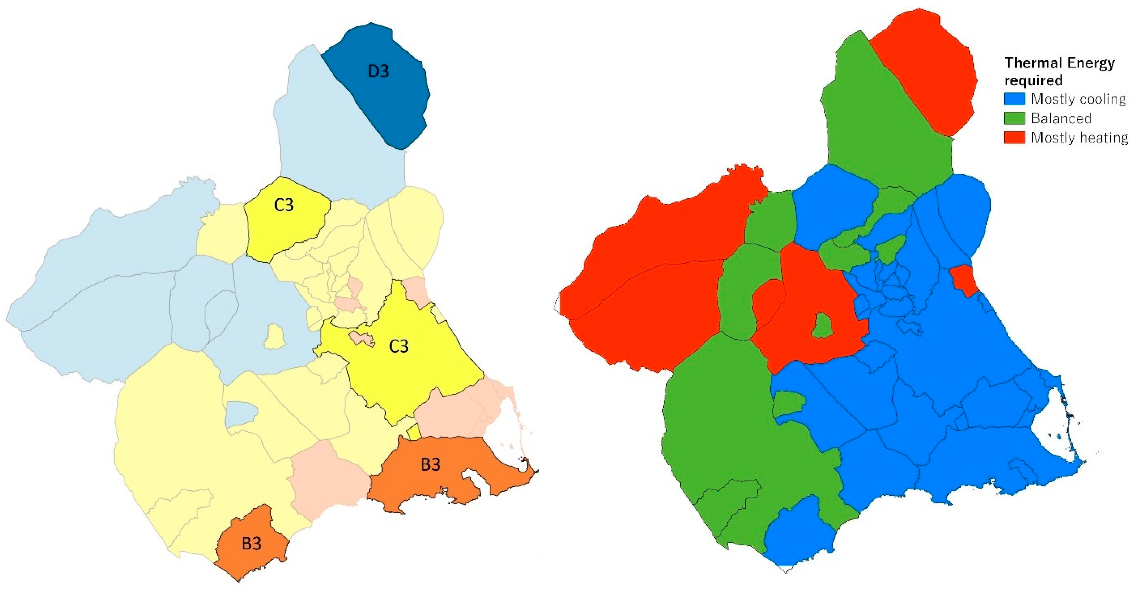
• Based on the climatic conditions, the average energy needs of the residential building stock were identified per municipality within the region. Depending on the climate zone, the heating needs vary from 3200 to 6200 kWh/year and the cooling needs vary from 3800 to 5200 kWh/year;
• Results showed that the cooling mode is the prevailing mode in the majority of the municipalities within the region, although the heating needs turned out to also be considerable. These conditions are relevant in the thermal efficiency of the SGE systems in the long term, as it may provoke the warming of the underground and the loss of efficiency in the future;
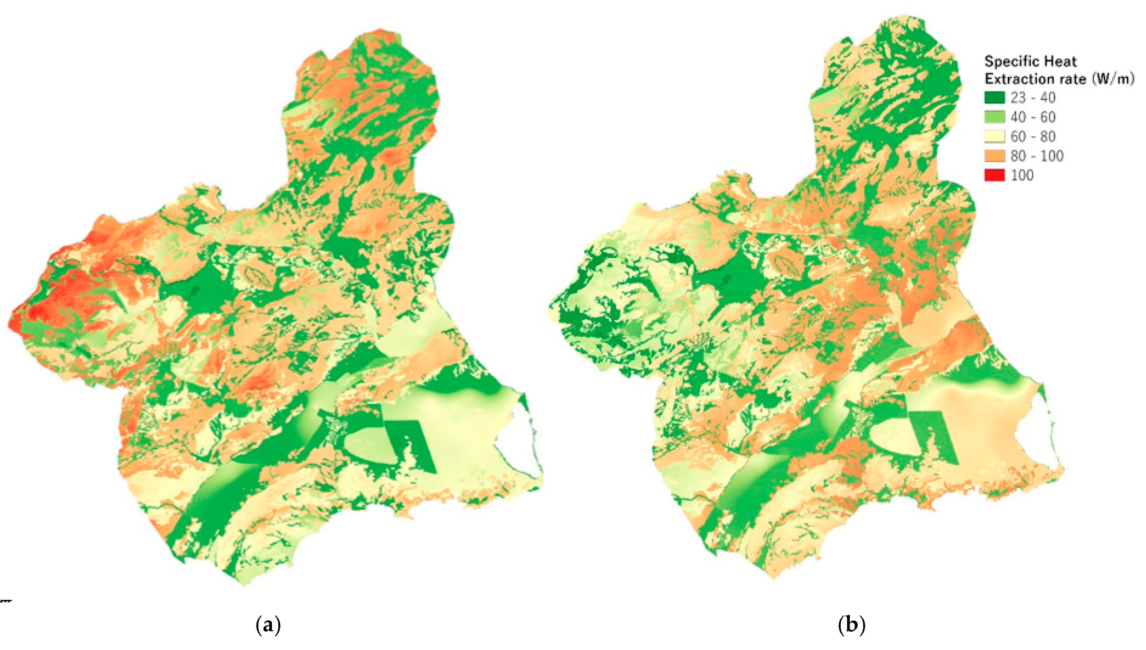
• Technical parameters of the GSHP to cover the required energy demand were also assessed. To this end, the sHe rate that the GSHP can supply at an hourly basis was estimated for heating and cooling separately. The sHe for heating varies from 17 to 87 W/m, with a regional average of 56.2 W/m, and 38 to 85 W/m for cooling, with 56.7 W/m as average. High sHe rate areas are different when considering the heating and cooling needs and are localized where the highest temperature difference between the heat carrier fluid and ambient temperature is located. sHe rates obtained here are slightly higher than those from VDI4640, although, here, operating hours are lower than in the VDI (1200 vs. 1800 to 2400);
• The sizing of the reference GSHP system for each municipality in order to cover the entire thermal loads was assessed, ranging from 4 to 7 kW. The combination of the power required and the sHe value allowed us to know that the BHE length of the reference system may vary between 45 to 410 m. Nevertheless, the mean value is 99 m, which usually varies ± 50 m;
• Drilling BHE costs were calculated using a fixed value of 50 €/meter, and the result shows that drilling cost varies from EUR 2300 to EUR 21,000, with a mean value of EUR 5000;
• The total cost of the reference GSHP was also calculated, which ranges between EUR 15,300 and EUR 34,000. A higher GSHP cost is found where higher associated energy demands are located. The GSHP payback period calculated shows that the investment can be recovered in between 8 and 20 years, with 11 years as an average. Considering a 10-year period, shallow geothermal energy production costs in the region vary from 0.13 to 0.18 €/kWh. Compared to the current electricity cost, which is by far the main primary energy used to produce H&C in the region, these prices represent an increment of 10 to 35%. It is worth highlighting that any public financial support was considered in the economic study;
• Finally, the environmental benefits of the use of the shallow geothermal potential in the region were brought to light. GHG emissions savings were associated with each climate zone: in B3 areas, 0.13 Tn of CO₂ as an average can be annually saved per GSHP system, 0.15 Tn in C3 and 0.16 Tn in C3 areas.

References

1. European Commission. An EU Strategy on Heating and Cooling. Communication from the Comission to the European Parliament, The Council, the European economic and Social Committee and the Comittee of the Regions; European Commission: Brussels, Belgian, 2016. [Google Scholar]
2. European Commission. Stepping up Europe’s 2030 climate ambition Investing in a climate-neutral future for the benefit of our people. J. Chem. Inf. Model. 2020, 53, 1689–1699. [Google Scholar]
3. Lund, J.W.; Boyd, T.L. Direct utilization of geothermal energy 2015 worldwide review. Geothermics 2016, 60, 66–93. [Google Scholar] [CrossRef]
4. IRENA. Rise of Renewables in Cities: Energy Solutions for the Urban Future; International Renewable Energy Agency: Abu Dabi, United Arab Emirates.
5. International Energy Agency (IEA) COVID-19. Exploring the Impacts of the COVID-19 Pandemic on Global Energy Markets, Energy Resilience, and Climate Change. Available online: https://www.iea.org/topics/covid-19 (accessed on 4 July 2021).
6. Gondal, I.A. Prospects of Shallow geothermal systems in HVAC for NZEB. Energy Built Environ. 2020, 2, 425–435. [Google Scholar] [CrossRef]
7. Maddah, S.; Goodarzi, M.; Safaei, M.R. Comparative study of the performance of air and geothermal sources of heat pumps cycle operating with various refrigerants and vapor injection. Alex. Eng. J. 2021, 59, 4037–4047. [Google Scholar] [CrossRef]
8. Badenes, B.; Sanner, B.; Pla, M.Á.M.; Cuevas, J.M.; Bartoli, F.; Ciardelli, F.; González, R.M.; Ghafar, A.N.; Fontana, P.; Zuñiga, L.L.; et al. Development of advanced materials guided by numerical simulations to improve performance and cost-efficiency of borehole heat exchangers (BHEs). Energy 2020, 201, 117628. [Google Scholar] [CrossRef]
9. Javadi, H.; Urchueguia, J.F.; Ajarostaghi, S.S.M.; Badenes, B. Numerical Study on the Thermal Performance of a Single U-Tube Borehole Heat Exchanger Using Nano-Enhanced Phase Change Materials. Energies 2020, 13, 5156. [Google Scholar] [CrossRef]
10. Ondreka, J.; Rüsgen, M.I.; Stober, I.; Czurda, K. GIS-supported mapping of shallow geothermal potential of representative areas in south-western Germany—Possibilities and limitations. Renew. Energy 2007, 32, 2186–2200. [Google Scholar] [CrossRef]
11. Noorollahi, Y.; Arjenaki, H.G.; Ghasempour, R. Thermo-economic modeling and GIS-based spatial data analysis of ground source heat pump systems for regional shallow geothermal mapping. Renew. Sustain. Energy Rev. 2017, 72, 648–660. [Google Scholar] [CrossRef]
12. Viesi, D.; Galgaro, A.; Visintainer, P.; Crema, L. GIS-supported evaluation and mapping of the geo-exchange potential for vertical closed-loop systems in an Alpine valley, the case study of Adige Valley (Italy). Geothermics 2018, 71, 70–87. [Google Scholar] [CrossRef]
13. García-Gil, A.; Vázquez-Suñe, E.; Alcaraz, M.M.; Juan, A.S.; Sánchez-Navarro, J.Á.; Montlleó, M.; Rodríguez, G.; Lao, J. GIS-supported mapping of low-temperature geothermal potential taking groundwater flow into account. Renew. Energy 2015, 77, 268–278. [Google Scholar] [CrossRef]
14. Schiel, K.; Baume, O.; Caruso, G.; Leopold, U. GIS-based modelling of shallow geothermal energy potential for CO2 emission mitigation in urban areas. Renew. Energy 2016, 86, 1023–1036. [Google Scholar] [CrossRef]
15. Ramachandra, T.V.; Shruthi, B.V. Spatial mapping of renewable energy potential. Renew. Sustain. Energy Rev. 2007, 11, 1460–1480. [Google Scholar] [CrossRef]
16. QGIS. Geographic Information System. Open Source Geospatial Foundation Project. 2019. Available online: https://www.qgis.org/es/site/ (accessed on 4 July 2021).
17. Casasso, A.; Sethi, R.G. POT: A quantitative method for the assessment and mapping of the shallow geothermal potential. Energy 2016, 106, 765–773. [Google Scholar] [CrossRef]
18. VDI 4640 Directive. Thermal Use of the Underground. Fundamentals, Approvals and Environmental Aspects. Available online: www.vdirichtlinien.de (accessed on 4 July 2021).
19. Erol, S. Estimation of Heat Extraction Rates of GSHP Systems under Different Hydrogelogical Conditions. Master’s Thesis, Universität Tübingen, Tübingen, Germany, 2011. [Google Scholar]
20. Staiti, M.; Angelotti, A. Design of Borehole Heat Exchangers for Ground Source Heat Pumps: A Comparison between Two Methods. Energy Procedia 2015, 78, 1147–1152. [Google Scholar] [CrossRef] [Green Version]
21. Gemelli, A.; Mancini Adriano, A.; Longhi, S. GIS-based energy-economic model of low temperature geothermal resources: A case study in the Italian Marche region. Renew. Energy 2011, 36, 2474–2483. [Google Scholar] [CrossRef]
22. UNE Normalización Española. UNE 100715-1. Diseño, Ejecución y Seguimiento de una Instalación Geotérmica Somera. 2014. Available online: https://www.une.org/encuentra-tu-norma/busca-tu-norma/norma?c=N0052899 (accessed on 4 July 2021).
23. DINOloket. Geological Survey of The Netherlands. Available online: https://www.dinoloket.nl/ (accessed on 4 July 2021).
24. Gwadera, M.; Larwa, B.; Kupiec, K. Undisturbed ground temperature-Different methods of determination. Sustainability 2017, 9, 2055. [Google Scholar] [CrossRef] [Green Version]
25. Good, E.J.; Ghent, D.J.; Bulgin, C.E.; Remedios, J.J. A spatiotemporal analysis of the relationship between near-surface air temperature and satellite land surface temperatures using 17 years of data from the ATSR series. J. Geophys. Res. Atmos. 2017, 122, 9185–9210. [Google Scholar] [CrossRef]
26. The Chartered Institution of Building Services Engineers (CIBSE). Degree-Days: Theory and Application; CIBSE: London, UK, 2006; ISBN 9781903287767. [Google Scholar]
27. Interreg Alpine Space GRETA Project. Local-Scale Maps of the NSGE Potential in the Case Study Areas; Interreg Alpine Space: Munich, Germany, 2018. [Google Scholar]
28. Sigfusson, B.; Uihlein, A. Geothermal Energy Status Report—JRC Science and Policy Reports. European Commission: Luxembourg, 2015; ISBN 978-92-79-44614-6. [Google Scholar]
29. Urchueguía, J.F.; Zacarés, M.; Corberán, J.M.; Montero, Á.; Martos, J.; Witte, H. Comparison between the energy performance of a ground coupled water to water heat pump system and an air to water heat pump system for heating and cooling in typical conditions of the European Mediterranean coast. Energy Convers. Manag. 2008, 49, 2917–2923. [Google Scholar] [CrossRef]
30. Geological Survey of Spain (IGME) Geology of Murcia Area. Available online: https://www.regmurcia.com/servlet/s.Sl?sit=c,365,m,108&r=ReP-16267-DETALLE_REPORTAJESPADRE (accessed on 4 July 2021).
31. Development Spanish Ministry. DB-HE Ahorro de Energía. Building Technical Code; Spanish Ministry of Housing: Madrid, Spain, 2019.
32. IDAE-Institute for Energy Diversification and Saving Project Sech-Spahousec. Analysis of the Energetic Consumption of the Residential Sector in Spain; IDAE: Madrid, Spain, 2016. [Google Scholar]
33. IGME Instituto Geológico y Minero Mapa Geológico de Murcia Escala 1:200.000. 2000. Available online: http://info.igme.es/cartografiadigital/geologica/Geologicos1MMapa.aspx?Id=Geologico1000_(1994) (accessed on 4 July 2021).
34. Ministerio para la Transición Ecológica y el Reto Demográfico. Red de Seguimiento del Estado Cuantitativo. Available online: https://www.miteco.gob.es/es/agua/temas/evaluacion-de-los-recursos-hidricos/red-oficial-seguimiento/ (accessed on 4 July 2021).
35. UAB. Iberian Peninsula Climatic Atlas. Available online: http://www.opengis.uab.es/wms/iberia/mms/index.htm (accessed on 4 July 2021).
36. AEMET. Climatic Data Analysis Software. Available online: http://www.aemet.es/es/portada (accessed on 4 July 2021).
37. Air-conditioning Spanish Association (ATECYR). Heating Needs in Murcia Region; Air-Conditioning Spanish Association (ATECYR): Murcia, Spain, 2015. [Google Scholar]
38. Rybach, L. Design and performance of borehole heat exchanger/heat pump design and performance of borehole heat exchanger/heat pump systems. Engineering 2000, 173–181, Corpus ID: 114429932. [Google Scholar]
39. Instituto para la Diversificación y Ahorro de la Energía. IDAE Síntesis del Estudio Parque de Bombas de Calor en España; IDAE: Madrid, Spain, 2016. [Google Scholar]
40. Spanish Transport and Operation Electricity Corporation (Red Eléctrica de España). Available online: https://www.ree.es/es (accessed on 4 July 2021).
Figure 1. GIS-based top-down methodology workflow.
Energies 14 05740 g001
Figure 2. Schematic overview of the GIS approach.
Energies 14 05740 g002
Figure 3. Digital elevation model and location of Region of Murcia.
Energies 14 05740 g003
Figure 4. Map of the water table level from the surface to 100 m depth. The points represent the piezometers considered in the area. Green points represent those considered for the map and dark points represent those dismissed for the map, as the level goes deeper than 100 m.
Energies 14 05740 g004
Figure 5. Map of thermal conductivity in the Region of Murcia based on UNE 100715 —1 values.
Energies 14 05740 g005
Figure 6. Map of the shallow geothermal potential for space heating (a) and space cooling (b) in the Region of Murcia with the G.POT method up to 100 m depth.
Energies 14 05740 g006aEnergies 14 05740 g006b
Figure 7. Climatic needs characterization. On the left, municipalities in the darker color with meteorological stations where HDD and CDD data are measured and, in lighter color, municipalities where HDD and CDD were estimated from those with real values. (Left) Climatic characterization based on the energy mode prevailing by municipality. In blue, municipalities where up to 75% are cooling needs; in green, municipalities where approximately half are for cooling and half for heating; and in red, municipalities where at least 75% of demand is for heating. Own elaboration.
Energies 14 05740 g007
Figure 8. Specific heat extraction (sHE) rate for cooling mode (a) and heating mode (b) estimated with G. POT method based on the hydrogeological and climatic conditions.
Energies 14 05740 g008
Figure 9. Power demanded to supply heating and cooling need by municipality (a) and BHE length required to supply these needs (b).
Energies 14 05740 g009
Figure 10. Drilling costs map. Costs are calculated on the basis of the BHE length required.
Energies 14 05740 g010
Figure 11. Map of GSHP payback period considering only the yearly space heating demand.
Energies 14 05740 g011
Figure 12. Map of the production cost of geothermal energy (€/kWh).
Energies 14 05740 g012
Figure 13. Map of GHG emissions savings per house (Tn/y) considering a complete migration of the energy residential sector to shallow geothermal.
Energies 14 05740 g013