Modeling and Optimization of Wind Turbines in Wind Farms for Solving Multi-Objective Reactive Power Dispatch Using a New Hybrid Scheme

Abstract

Reactive Power Dispatch is one of the main problems in energy systems, particularly for the power industry, and a multi-objective framework should be proposed to solve it. In this study, we present a multi-objective framework for the optimization of wind turbines in wind farms. We investigate a new combined optimization method with Chaotic Local Search, Fuzzy Interactive Honey Bee Mating Optimization, Data-Sharing technique and Modified Gray Code for discrete variables. We use the proposed model to select optimal energy system parameters. The optimization process is based on simultaneous optimization of three functions. Finally, we improve a new method based on Pareto-optimal solutions to select the best one among all candidate solutions. The presented model and methodology are validated on energy systems with wind turbines. The evaluated efficiency is compared with the real system.

1. Introduction

Reactive Power Dispatch (RPD) is tightly coupled to bus voltages throughout a distribution power network [1,2,3,4,5,6,7,8,9,10,11,12]. Hence, it has a noteworthy effect on system security [13,14,15,16,17,18,19,20,21,22,23,24]. One of the important reasons for some of the recent blackouts in the power distribution systems around the world, such as those that occurred in Canada, the United States, Sweden, Denmark, and Italy, was reported as inadequate reactive power resources of the system, resulting in voltage collapse [25,26,27,28,29,30,31,32,33,34,35,36]. The RPD problem is a non-differentiable optimization problem with a multidimensional search space. This is due to the size of control parameters, which minimize the non-commensurable and conflicting objective functions via finding control variables while fulfilling certain system constraints [37,38,39,40,41,42,43,44,45,46,47,48]. Renewable systems, including hybrid renewable energy systems, have increased quickly in recent years. Principally, wind energy penetration (from large wind farms) is much larger compared with other renewable energy sources worldwide and is one of the most promising options for future energy [49,50]. Large-scale wind farms impact the power network in 2 ways [51,52,53,54,55,56,57,58,59,60,61,62]:

(i)

Areas with valuable wind energy are used for power network terminals [63,64,65,66,67,68,69,70];

(ii)

Wind energy has inherent uncertainties regarding the wind speed variable.

1.1. Literature Review

Recently, a large number of studies have been devoted to this problem of energy power systems and solutions have been presented for RPD problems. Nonlinear programming (NLP), linear programming (LP) and quadratic programming (QP) methods have been applied to solving RPD problems [71,72,73,74,75,76,77,78,79,80]. Many models have been presented in previous research studies [81,82,83,84,85,86,87,88,89,90] and have been applied to resolving the RPD problem. Optimization models used in a distributed generation have been found to be important [90,91,92,93,94,95]. In [96], optimization models of wind power generation were used to select wind turbine (WT) points in wind farms (WF). However, analysis has shown that when the objective function is epistatic, numbers of optimized variables are large, and the above-mentioned techniques’ efficiency is degraded to select global solutions, as well as results that do not approach the global optimum.

1.2. Motivations and Contributions

The important aims of this study are as follows:

(i)

We present power requirements for Wind Turbine to find active power control.

(ii)

(We propose a power dispatch model for wind farms via HBMO search.

(iii)

We propose some modifications in discrete search and local and global search.

(iv)

We propose a procedure based on the Technique for Order of Preference by Similarity to Ideal Solution (TOPSIS) to select a compromise solution via fuzzy interactive honey bee mating optimization (FIHBMO).

(v)

We test the efficiency of the mentioned method via simulations and validated using available data.

In Section 2 and Section 3, we introduce the RPD formulation with and without the WT Effect. In Section 4, we introduce the proposed scheme. We detail the application of FIHBMO to the proposed problem in Section 5. Results are compared to previous works in Section 6, and finally, Section 7 concludes with the results of this paper.

2. Problem Formulation without WT Effect

The power system’s goals are voltage stability and deviation, system transmission loss and security. Commonly, the RPD method is presented as follows.

2.1. Problem Objectives

• Objective 1: Power loss minimization

Transmission losses are economic losses, and minimization of them is important. Transmission losses for bus voltages are presented via Newton–Raphson:

$$J_1={\mathrm{P}}_{loss}(x,u)={\displaystyle \sum _{k=1}^{N_L}{g}_k[V_i^2}+V_j^2-2V_i{V}_j\cos ({\theta }_i-{\theta }_j)]$$

(1)

The g is line conductance, V and θ are line voltage and angles, N_D is power demand bus, N_j is bus number adjacent to bus j. P_loss is transmission power loss.

• Objective 2: Voltage deviation (VD) minimization

The second function of RPD is presented as follows:

$$J_2=VD(x,u)={\displaystyle \sum _{i=1}^{Nd}|V_i-1.0|}$$

(2)

The N_d is the load bus number.

• Objective 3: L-index voltage stability minimization

Voltage collapse is abrupt [95,96,97]. L-index, Lj of the bus, is presented via:

$$\left\{\begin{array}{l}{L}_j=\left|1-{\displaystyle \sum _{i=1}^{N_{PV}}{F}_{ji}\frac{V_i}{V_j}}\right|,j=1,2,\dots ,N_{PQ}\\ F_{ji}=-{[Y_1]}^{-1}[Y_2]\end{array}\right.$$

(3)

The N_PV and N_PQ are the number of PV and PQ bus, and Y₁ and Y₂ are sub-matrices of Y_BUS that are produced after segregation of PQ and PV bus bar, as presented in Equation (4):

$$\left[\begin{array}{l}{I}_{PQ}\\ I_{PV}\end{array}\right]=\left[\begin{array}{l}\begin{array}{cc}{Y}_1& Y_2\end{array}\\ \begin{array}{cc}{Y}_3& Y_4\end{array}\end{array}\right]\left[\begin{array}{l}{V}_{PQ}\\ V_{PV}\end{array}\right]$$

(4)

The L for system stability is presented via:

$$L=\max (L_j),j=1,2,\dots ,N_{PQ}$$

(5)

The objective function is obtained via:

$$J_3=VL(x,u)=L_{\max }$$

(6)

2.2. Objective Constraints

• Constraints 1: Equality Constraints

The constraints for the bus are obtained via:

$$\left\{\begin{array}{l}{P}_{G_i}-P_{D_i}=V_i{\displaystyle \sum _{j=1}^{N_B}{V}_j[G_{ij}\cos ({\theta }_i-{\theta }_j)+B_{ij}\sin ({\theta }_i-{\theta }_j)]}\\ Q_{G_i}-Q_{D_i}=V_i{\displaystyle \sum _{j=1}^{N_B}{V}_j[G_{ij}\sin ({\theta }_i-{\theta }_j)-B_{ij}\cos ({\theta }_i-{\theta }_j)]}\end{array}\right.$$

(7)

The NB is bus number; Q_Gi is reactive power of bus; P_Di and Q_Di are load real and reactive power. The G_ij and B_ij are transfer conductance and susceptance between buses i and j. The V is voltage magnitude and θ is voltage angle at buses.

• Constraints 2: Generation Capacity Constraints

Generator power and bus voltage are obtained via:

$$Q_i^{\min }\le Q_i\le Q_i^{\max },v_i^{\min }\le v_i\le v_i^{\max }$$

(8)

where Q_i^min _and Q_i^max are power minimum and maximum, and v_i^min and v_i^max are ith transmission line voltage. The thermal curve is presented in Figure 1.

• Constraints 3: Line flow constraints

Here, RPD solution is discussed via the proposed algorithm, and this constraint is presented as follows:

$$\left|S_{Lf,k}\right|\le S_{Lf,k}^{\max },k=1,2,\dots ,L$$

(9)

The $S_{Lf,k}^{\max }$ is the flow limit, and L is lines [77].

• Constraints 4: Discrete control variables

The shunt susceptance (B_sh) and transformer tap settings (T_i) values are obtained as discrete values, and they are restricted via limits in Equation (10):

$$\left\{\begin{array}{l}{T}_i^{\min }\le T_i\le T_i^{\max }\\ B_{s{h}_i}^{\min }\le B_{s{h}_i}\le B_{s{h}_i}^{\max }\end{array}\right.$$

(10)

2.3. Problem Formulation

RPD is represented by:

$$\begin{array}{l}{J}_{Final}=\underset{P_G}{\min }[VL(x,u),VD(x,u),{\mathrm{P}}_{loss}(x,u)]\\ subject\hspace{1em}to:\\ g(x,u)=0\\ h(x,u)\le 0\\ where,{\mathrm{x}}^{\mathrm{T}}{=\left[\right[\mathrm{V}}_{\mathrm{L}}{]}^{\mathrm{T}}{, [\mathrm{Q}}_{\mathrm{G}}{]}^{\mathrm{T}}{, [\mathrm{S}}_{\mathrm{L}}{]}^{\mathrm{T}}],\\ \hspace{1em}\hspace{1em}\hspace{1em}{\mathrm{u}}^{\mathrm{T}}{=\left[\right[\mathrm{V}}_{\mathrm{G}}{]}^{\mathrm{T}}{, \left[\mathrm{T}\right]}^{\mathrm{T}}{, [\mathrm{Q}}_{\mathrm{C}}{]}^{\mathrm{T}}]\end{array}$$

(11)

The g and h are equality and inequality constraints. [V_L], [Q_G], and [S_L] are vectors of load bus voltages, generator outputs, and transmission line loading. [V_G] and [Q_C] are vectors of generator bus voltages and reactive compensation devices. The x and u are control variable vectors.

3. Problem Formulation with Wind Turbine Effect

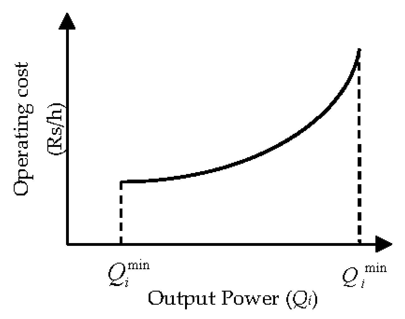
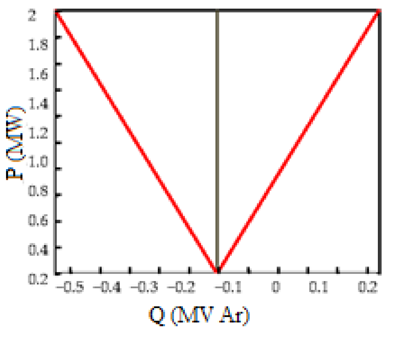
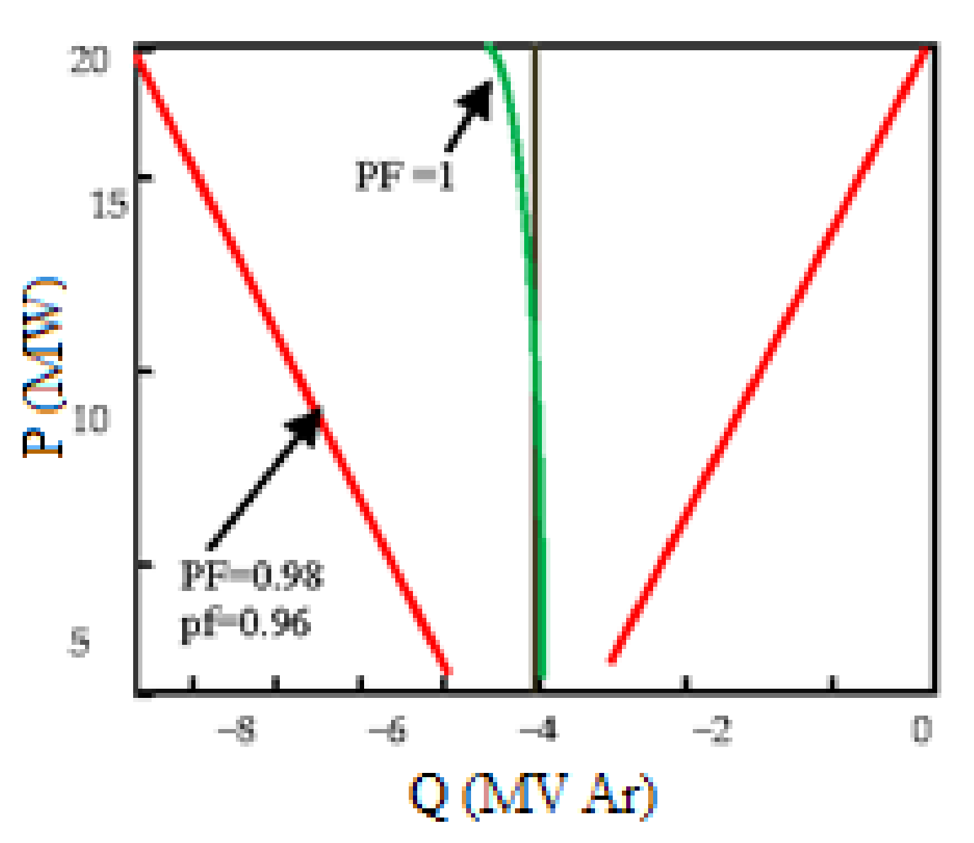
3.1. Power Capacity in Wind Farms

The WT expansion concepts are important in variable speed wind turbines, and DFIG usually pertains to wind generation technology [98].

Here, the double-feed induction generator (DFIG) method is used, and P–Q qualities of WTs are presented in Figure 2. The data of wind turbine Gamesa WT G80-2.0MW is given in [99], and in this WT, the power ability is bounded (red color). WF P-Q properties are similar to WTs but transferred to the capacitive side (green color) which is presented in Figure 3.

When WF takes capacitive power in low power WTs are changed to inductive.

3.2. Objective Function

Control of STATCOM and capacitor bank for RPD optimization via FIHBMO algorithm are used. The suggested fitness is taken to minimize power loss via WF cables as follows:

$${\mathrm{Minimize} \mathrm{J}(\mathrm{Var}}_{\mathrm{x}}{,\mathrm{Var}}_{\mathrm{y}}{) =\mathrm{Min} \mathrm{P}}_{\mathrm{losses}}$$

(12)

The Var_y represents transformer tap, and Var_x refers to dependent variables, which are WT power outputs. The j is optimized variables and each i is the solution.

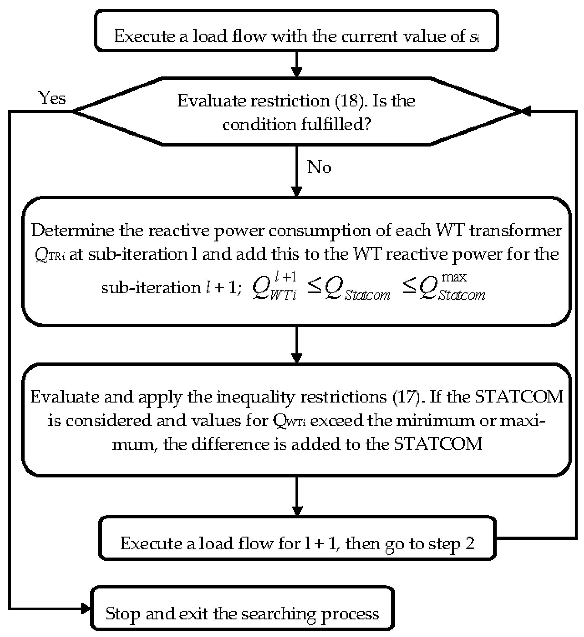
3.3. Objective Constraints

The WT power, transformers tab, and STATCOM are limited via their minimum and maximum capacity, respectively:

$$Q_{W{T}_i}^{\min }\le Q_{W{T}_i}\le Q_{W{T}_i}^{\max },i=1,2,\dots ,N_G$$

(13)

$$T_i^{\min }\le T_i\le T_i^{\max }$$

(14)

$$Q_{Statcom}^{\min }\le Q_{Statcom}\le Q_{Statcom}^{\max }$$

(15)

where

The power prerequisite in PCC models is as follows:

$$Q_{PCC}^{*}=Q_{PCC}^{meas}$$

(16)

where $Q_{W{T}_i}$, $Q_{Statcom}$ and $T_i$ are wind reactive power, STATCOM output and transformers tab position, respectively. Solutions searching are employed, and limitations are presented via:

$$S_i^{k+1}=\left\{\begin{array}{ll}{S}_i^k+v_i^{k+1},& S_i^{\min }\le S_i^k+v_i^{k+1}\le S_i^{\max }\\ S_i^{\min },& S_i^{\min }>S_i^k+v_i^{k+1}\\ S_i^{\max },& S_i^k+v_i^{k+1}>S_i^{\max }\end{array}\right.$$

(17)

where S indicates the feasible solution. With the above equation, the inequality restraints are satisfied, and equality restraint (16) remains solved. To decrease the CPU time searching, the equality constraint is increased, and error is presented via:

$$|Q_{PCC}^{*}-Q_{PCC}^{meas}|<\epsilon$$

(18)

4. The Suggested Scheme

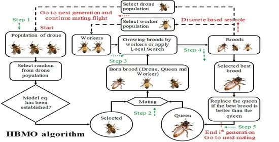
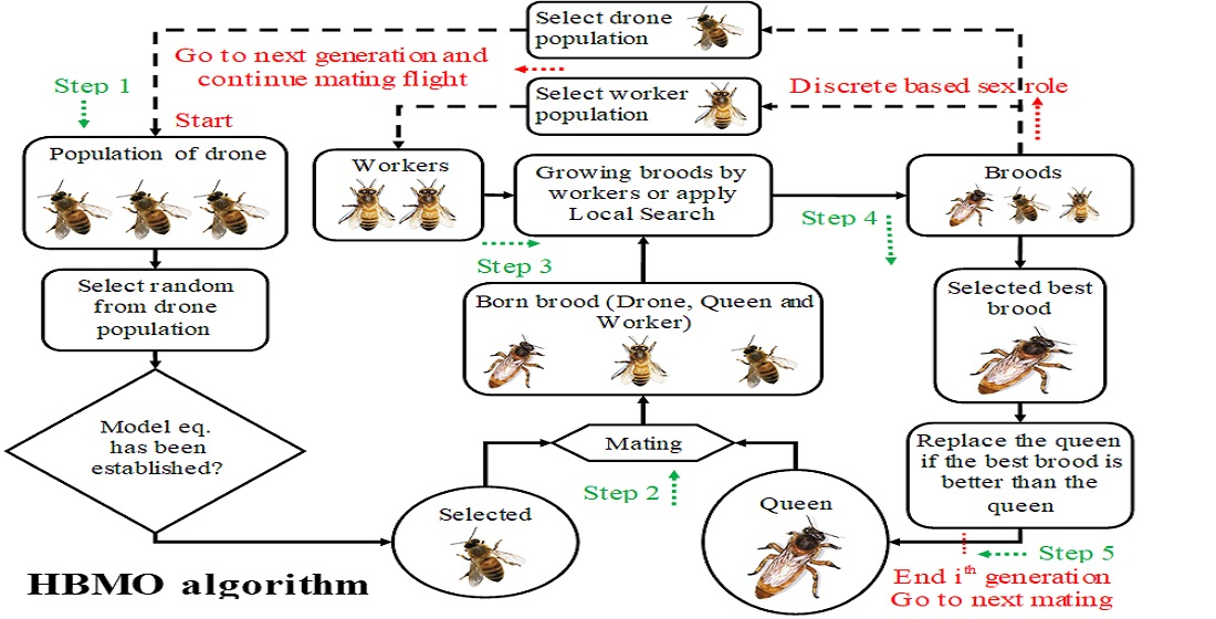
4.1. Briefly Review of Standard HBMO Algorithm

The honeybee has a single queen and thousands of workers [100]. For algorithm development, workers are limited to squab care, which acts to increase the broods. The drone mates use the following function [101]:

$$prob(Q,D)=e^{\frac{-\Delta (f)}{S(t)}}$$

(19)

The S(t) and E(t) decay by these equations:

$$S\left(\mathrm{t}+1\right)={\alpha }_{HBMO}\times S\left(\mathrm{t}\right)$$

(20)

$$E\left(\mathrm{t}+1\right)=E\left(\mathrm{t}\right)-{\mathsf{\gamma }}_{HBMO}$$

(21)

where Mate_Prob(Q,D) is the probability function of adding the sperm of drone D to the spermatheca of queen Q. ∆(f) is the absolute difference between the fitness of D (i.e., f(D)) and the fitness of Q (i.e., f(Q)). S(t) is queen’s speed at time t. E(t) is queen’s energy at time t.

The HBMO steps are the following:

Step 1:

This step is controlled by several parts and the start of the HBMO procedure. Then, the drone is selected from generated broods.

Step 2:

Algorithm is started via Equation (19), and the mating flight is finished when spermatheca is complete.

Step 3:

Broods are produced via Equation (22), and they transfer genes of drones and queen to jth, which is obtained via

$$brood=drone+{\beta }_{HBMO}(queen-drone),{\beta }_{HBMO}=\left(0,1\right)$$

(22)

Step 4:

The community of broods increases by applying the mutation operators as follows:

$$\begin{array}{l}broo{d}_i^k=broo{d}_i^k\pm ({\delta }_{HBMO}+{\epsilon }_{HBMO})broo{d}_i^k\\ 0<{\epsilon }_{HBMO},{\delta }_{HBMO}<1\end{array}$$

(23)

β_HBMO is the decreasing factor, ε_HBMO is the growing factor and δ_HBMO is the growth factor.

Step 5:

If finish criteria are satisfied, the algorithm is complete; if it happens for the old criteria, go to stage 2. Otherwise, choose the current one and go to stage 2.

4.2. Fuzzy Chaotic Interactive HBMO

The HBMO includes a flexible structure for developing global exploration potential. The HBMO algorithm utilizes the independent randomly such that it affects algorithm stochastic nature Equation (22). To overcome this problem in this study, the Newtonian law of universal gravitation is added to Equation (22) as follows:

$$\begin{array}{l}{F}_{i{k}_j}=G\frac{F(paren{t}_i)\times F(paren{t}_k)}{{(paren{t}_{kj}-paren{t}_{ij})}^2}.\frac{paren{t}_{kj}-paren{t}_{ij}}{|paren{t}_{kj}-paren{t}_{ij}|},\\ broo{d}_{ij}(t+1)=paren{t}_{ij}(t)+F_{i{k}_j}.[paren{t}_{ij}(t)-paren{t}_{kj}(t)]\end{array}$$

(24)

where, F(parent_i) is the fitness value of the queen i. F(parent_k) is the fitness value of the drone k. In IHBMO, the gravitational force attracts drones to others, and if premature convergence occurs, there is no recovery in the algorithm. So, a new operator is added to IHBMO to improve its flexibility in solving problems. Then, a new operator is presented:

$$c_{i+1}^j=\left\{\begin{array}{c}2c_i^j\times (1+\frac{{\mathrm{g}}_{best}^{k-1}}{{\mathrm{g}}_{best}^k})\times \cos (2\pi \frac{{\mathrm{g}}_{best}^{k-1}}{{\mathrm{g}}_{best}^k}),0.5<c_i^j\le 1\\ 0.1c_i^j\times (1-\cos \left(\right(1+\frac{{\mathrm{g}}_{best}^{k-1}}{{\mathrm{g}}_{best}^k}\left)\right)),0<c_i^j\le 0.5\end{array}\right.$$

(25)

N_chaos is the number of individuals for CLS. g_j^best is the best answer for the jth iteration. Where C_i^j is the chaos variable. The ${\mathrm{g}}_{best}^{k-1}/{\mathrm{g}}_{best}^k$ reports that fine-tuning is necessary to obtain a gyration sequence. The chaotic search on IHBMO is obtained via the following steps.

Step 1:

Produce the initial chaos population in CLS.

$$\begin{array}{l}{X}_{cls}^0={[X_{cls,0}^1,X_{cls,0}^2,\dots ,X_{cls,0}^{Ng}]}_{1\times N_g}\\ c{x}_0=[c{x}_0^1,c{x}_0^2,\dots ,c{x}_0^{Ng}]\\ c{x}_0^j=\frac{X_{cls,0}^j-P_{j,\min }}{P_{j,\max }-P_{j,\min }},j=1,2,\dots ,Ng\end{array}$$

(26)

Chaos variable is obtained via

$$\begin{array}{l}{X}_{cls}^i={[X_{cls,i}^1,X_{cls,i}^2,\dots ,X_{cls,i}^{Ng}]}_{1\times N_g},i=1,2,\dots ,N_{chaos}\\ x_{cls,i}^j=c{x}_{i-1}^j\times (P_{j,\max }-P_{j,\min })+P_{j,\min },j=1,2,\dots ,N_g\end{array}$$

(27)

Step 2:

Chaotic variables

$$\begin{array}{l}c{x}_i=[c{x}_i^1,c{x}_i^2,\dots ,c{x}_i^{Ng}],i=0,1,2,\dots ,N_{choas}\\ c{x}_{i+1}^j=base CLS\hspace{1em}j=1,2,\dots ,Ng\\ c{x}_0^j=rand(0)\end{array}$$

(28)

The Rand [0,1] produces a number from 0 to 1.

Step 3:

Map variables

Step 4:

Chaotic variables to variables

Step 5:

Solution via variables.

To develop the performance of IHBMO, the ε_HBMO and δ_HBMO adapt via

$$\begin{array}{l}{\epsilon }_{HBMO}^{iter+1}={\epsilon }_{HBMO}^{iter}+\Delta {\epsilon }_{HBMO}^{iter},\Delta {\epsilon }_{HBMO}^{iter}\in [-1,1]\\ {\delta }_{HBMO}^{iter+1}={\delta }_{HBMO}^{iter}+\Delta {\delta }_{HBMO}^{iter},\Delta {\delta }_{HBMO}^{iter}\in [-1,1]\end{array}$$

(29)

$\Delta {\epsilon }_{HBMO}^{iter}$ and $\Delta {\delta }_{HBMO}^{iter}$ are obtained via a fuzzy mechanism as follows:

$$Nor\_Fi{t}^{iter}=\frac{F(g_{best}^{iter})-F_{\min }}{F_{\max }-F_{\min }}\in [0,1]$$

(30)

Nor_Fit^iter, ε_HBMO, and δ_HBMO contain input variables, and changes in growth are output variables. To select the best growth factors, the triangular functions are considered.

4.3. Modified Gray Code (MGC)

Gray code is suggested via Frank Gray for shaft encoders [102], and its mathematical methods are presented in [103]. In integer parameter m ∈ N, [m] shows set {0, 1, …,m}, and in n-tuple, b ∈ Nn:

• [b] denotes the produce set [b₁] × [b₂]×· · ·×[b_n], and
• $\left|\right|b\left|\right|={\displaystyle {}_{i=1}^n{b}_i}$.

The MGC in creation [b], shown here by G_n(b), is obtained via:

$$G_n\left(b\right)=\left\{\begin{array}{l}0,if\hspace{1em}n=0\\ 0G_{n-1}\left(b’\right),1\overline{G_{n-1}\left(b’\right),}2G_{n-1}\left(b’\right)\\ \hspace{1em}\hspace{1em}\hspace{1em},\dots ,G_{n-1}^{’}\left(b’\right),f n>0\end{array}\right.$$

(31)

$b^{’}=b_2{b}_3\dots b_n$ and $\overline{G_{n-1}\left(b’\right)}$ are reverse for $G_{n-1}\left(b’\right)$, and $G_{n-1}^{’}\left(b’\right)$ is $G_{n-1}\left(b’\right)$. Two-tuple $G_n\left(b\right)$ differs by +1 or −1; note that in Gray code method [28], a new ordering scheme linearly builds piecewise and more precisekly, since overall, J_Final is smoother and “jumpy”. B_sh (shunt) and T tap include a small capacity change for numbers, and J_Final function is obtained via one variable; a Gray code assists in reducing piecewise the J_Final function to one-dimension.

4.4. Non-Dominated Sorting (NDS)

In sorting, the agent chooses method in the population or not in it:

$$Obj.1[i]<Obj.1[j]\hspace{1em}and\hspace{1em}Obj.2[i]<Obj.2[j],i\ne j$$

(32)

This method continues until shared fitness is obtained, and these values are obtained via

$$\mathrm{Share}\left(d_{ij}\right)=\left\{\begin{array}{ll}1-{(\frac{d_{ij}}{{\mu }_{share}})}^2,& if\hspace{1em}{d}_{ij}<{\mu }_{share}\\ 0,& otherwise\end{array}\right.$$

(33)

$$d_{ij}=\sqrt{{\displaystyle \sum _{a=1}^{P_1}{(\frac{x_s^i-x_s^j}{x_s^{\max }-x_s^{\min }})}^2}}$$

(34)

The p₁ refers to variable numbers, x_s is the sth variable, and µ_share is the maximum distance between agents, and Nichecount (N) is obtained via

$$Nichecoun{t}_i={\displaystyle \sum _{j=1}^N\mathrm{Share}\left(d_{ij}\right)}$$

(35)

A.

TOPSIS mechanism

A fuzzy set is obtained to handle the dilemma; let (R_ij) be the efficiency rating of X_j with respect to A_i. To obtain objective weights via entropy, a model matrix is needed for each A_j using the following equation:

$$P_{ij}=\frac{R_{ij}}{{\displaystyle \sum _{p=1}^n{R}_{pj}}},\left\{\begin{array}{l}i=1,2,\dots ,N_p\\ j=1,2,\dots ,N_o\end{array}\right.$$

(36)

A normalized decision matrix showing alternative performance is obtained via:

$$P=\left[\begin{array}{cccc}{P}_{11}& P_{12}& \dots & P_{1m}\\ P_{21}& P_{22}& \dots & P_{2m}\\ ⋮& ⋮& \ddots & ⋮\\ P_{n1}& P_{n2}& \dots & P_{nm}\end{array}\right]$$

(37)

The decision quantity is obtained Equation (37), and for Aj (j = 1, 2, …, m), it can be obtained as follows:

$$e_j=\frac{-1}{\ln n}{\displaystyle \sum _{i=1}^n{P}_{ij}\ln P_{ij}}$$

(38)

The d_j of the average intrinsically controls for Aj via this equation:

$$d_j=1-e_j$$

(39)

The objective weights for Aj are:

$$w_j=d_j/{\displaystyle \sum _{k=1}^m{d}_k}$$

(40)

v_ij was calculated via:

$$v_{ij}=w_j{P}_{ij}$$

(41)

The subsequent step is aggregated to generate the performance of Aj, which it obtains via:

$$\left\{\begin{array}{l}{A}^{+}=(\max (v_{i1})\max (v_{i2})\dots \\ \hspace{1em}\hspace{1em}\hspace{1em}\hspace{1em}\hspace{1em}\hspace{1em}\hspace{1em}\max (v_{im}))=(v_1^{+},v_2^{+},\dots ,v_m^{+})\\ A^{-}=(\min (v_{i1})\min (v_{i2})\dots \\ \hspace{1em}\hspace{1em}\hspace{1em}\hspace{1em}\hspace{1em}\hspace{1em}\hspace{1em}\min (v_{im}))=(v_1^{-},v_2^{-},\dots ,v_m^{-})\end{array}\right.$$

(42)

A⁺ and A⁻ are the + and—solution, and alternatives are obtained via:

$$\begin{array}{l}{d}_j^{+}=\left\{{\displaystyle \sum _{i=1}^m(v_{ji}-v_i^{+})}\right\},j=1,2,\dots ,n\\ d_j^{-}=\left\{{\displaystyle \sum _{i=1}^m(v_{ji}-v_i^{-})}\right\},j=1,2,\dots ,n\end{array}$$

(43)

The relative closeness for Xj in A⁺ is obtained via:

$$C_j=\frac{d_j^{-}}{d_j^{-}+d_j^{+}},j=1,2,\dots ,n$$

(44)

The ${{\displaystyle d}}_j^{-}$ and ${{\displaystyle d}}_j^{+}$ ≥0 and C_j ∈ [0, 1].

The X_j was closer to A⁺ and steps need via this models:

Step 1:

Select pareto-optimal for functions.

Step 2:

Find attributes for cost.

Step 3:

List pareto-optimal.

Step 4:

Compute significance by Equation (40).

Step 5:

Made P_ij and v_ij.

Step 6:

Compute A⁺, A⁻.

Step 7:

Pareto-optimal and select C_j for maximum ranking.

B.

Data Sharing (DS)

Usage of optimizers is feasible to guide engineers. DS consider D drones, S1, S2, …, and SD in N to optimize M functions. The f₁ and f₂ are obtained via D₁ and D₂, and drones are obtained via respective functions. The D₂ queen is usedto obtain a new D₁ queen colony, and X₁ queen is used to obtain D₂ queen.

5. Applying the FIHBMO to the Proposed Problem

Here, the application of the suggested model for solving RPD is illustrated. The process of RPD optimization using the proposed technique is as follows:

Step 1:

The population of state variables is randomly produced. It can be calculated via:

$$D=[D_1,D_2,D_3,\dots ,D_n]\hspace{1em}\hspace{1em}{D}_i=(d_i^1,d_i^2,\dots ,d_i^m)$$

(45)

The D_i is calculated.

Step 2:

Randomly produce population of bees for variables.

Step 3:

Calculate functions and sort the population and data for fitness.

Step 4:

Use the suggested method for the best solution obtained for CLS, when the best solution is obtained via CLS as a new solution.

Step 5:

When broods are produced, solutions are improved with a mutation method.

Step 6:

If the iteration number obtains its maximum, the algorithm is finished; go to step 2.

The process of the algorithm is reported in Figure 4.

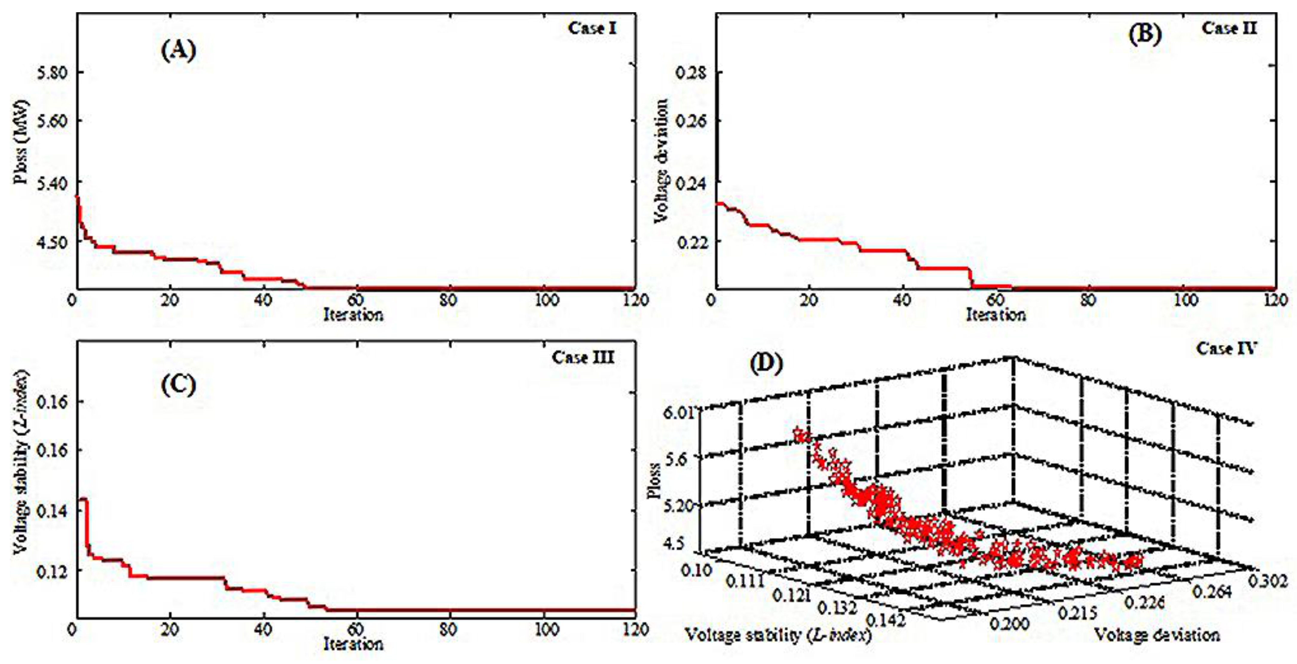
6. Simulation and Discussion

The proposed technique was applied in MATLAB(9.5/Mathworks, New York, NY, USA) to solve RPD, and simulations were done using a computer. To evaluate the effectiveness and robustness of this strategy, simulations were done for systems and in different cases using the following scenarios:

Scenario I: RPD without the effect iof wind.

Scenario II: Classic RPD in the presence of wind farms.

Scenario III: Proposed optimized dispatch based on Section 3.

6.1. Scenario I: RPD without Effect of WT

For this subsection, the suggested algorithm pf IEEE 30-bus was used, as presented in Figure 5, for obtaining algorithm suitability via the system in [104,105,106,107,108]. The output list is in

Table 1. Output Control Variables Obtained After Optimization For IEEE 30 Bus.

Control Variable Settings	Case I in Scenario I	Case II in Scenario I	Case III in Scenario I	Case IV in Scenario I
	Proposed Method	Proposed Method	Proposed Method	Proposed Method
V1 p.u	1.0919	1.0509	1.0831	1.0812
V2 p.u	1.0094	0.9552	1.0584	0.9254
V5 p.u	0.9277	1.0359	1.0919	1.0827
V8 p.u	0.9299	1.0310	1.0311	1.0265
V11 p.u	0.9515	0.9325	0.9071	0.9195
V13 p.u	1.0681	0.9238	1.0698	0.9557
T11	0.9509	0.9997	1.0868	1.0094
T12	1.0629	1.0919	1.0357	1.0915
T15	0.9487	0.9681	1.0515	1.0930
T36	1.0859	1.0171	1.0486	0.9315
QC10 p.u	2.9765	0.0448	4.9784	4.0941
QC12 p.u	3.9393	0.0503	4.0311	4.0914
QC15 p.u	2.9502	3.9510	3.9342	3.9971
QC17 p.u	2.0232	2.0012	4.0412	3.0601
QC20 p.u	1.0662	1.0514	5.000	0.9108
QC21 p.u	1.0171	1.0507	5.000	1.0062
QC23 p.u	1.0099	0.9761	5.000	1.0558
QC24 p.u	1.0834	1.0136	5.000	1.0868
QC29 p.u	1.0662	0.9152	5.000	0.9266
Power losses MW	4.4433	6.6423	6.661	4.9033
voltage deviations p.u	0.8343	0.0453	0.894	0.2432
Lmax	0.1332	0.1343	0.118	0.1332

.

To find the effectiveness for the suggested model, the four cases are suggested as follows:

Case (I) Function of real power losses is suggested (Figure 6A).

Case (II) Function of improvement voltage is suggested (Figure 6B).

Case (III) System was suggested as voltage stability (L-index) (Figure 6C).

Case (IV) Constraints were used for voltage stability and profile and transmission loss constraints (Figure 6D).

Results confirmed the potential of the suggested model for solving a real-world constrained optimization problem.

The results of the analyzed cases are reported in

Table 2. Comparison of transmission losses for different algorithms based on the optimization of the IEEE 30-bus system. Reproduced from [109], International Research Publication House: 2010.

Compared Item	SGA [109]	PSO [109]	HAS [109]	FIHBMO
Best Ploss (MW)	4.9408	4.9239	4.9059	4.9876
Worst Ploss (MW)	5.1651	5.0576	4.9653	5.8755
Average Ploss (MW)	5.0378	4.9720	4.9240	4.4356
Psave (%)	16.07	17.02	17.32	17.43

.

The FIHBMO was applied to 30-bus.

The transmission losses were reduced from 5.934 MW to 4.9593 MW via the proposed model. Data for the reduction system are compared to methods in [106,107]. In these methods, CLPSO is used for solving the optimization problem.

Table 3. Comparison of the proposed method with the literature results. Reproduced from [106], Elsevier: 2009.

Solving with Constraints According to [106]
Method	CLPSO [106]	EP [31]	CGA [106]	AGA [106]	PSO [106]
Ploss	5.988	4.963	4.980	4.926	4.8136
Method	CLPSO [106]	HSA [108]	HBMO	FIHBMO
Ploss	4.7208	4.7624	4.7693	4.432

shows the RPD solution if four compensation devices are installed after changing constraints in [108], and the problem was solved in comparison to SARCGA.

Moreover, the results of solving the RPD problem are reported in

Table 4. Comparison of the proposed method with the literature results. Reproduced from [106], Elsevier: 2009 and from [107] Elsevier: 2011.

Solving with Constraints According to [105]		Solving with Constraints According to [107]
Method	Power Loss	Method	Power Loss
PSO [108]	4.6723	PSO [11]	5.092
HAS [108]	4.6403	HAS [108]	5.007
SARCGA [107]	4.5913	GQ-GA [110]	5.04
GSA [109]	4.5143	DE [111]	5.011
BBO [112]	4.551	IPM [111]	5.101
FIHBMO	4.432	FIHBMO	4.989

. The FIHBMO has better problems, and data in FIHBMO are simple and acceptable in comparison to GA and PSO.

The results indicate that the suggested model has superiority and better results for power loss and solution quality than other models.

6.2. Scenario II: Classic RPD in WF

WF has 403 node [113,114,115,116,117,118,119,120,121], and only 42 nodes are presented in Figure 7.

Table 5. Compared results of reactive power optimization in wind farms. Reproduced from [39], Springer: 2020.

Project	Investment of Reactive Power Compensation (Million Yuan)	The System Loss(kW)
		V = 4m/s	V = 8m/s	V = 12m/s
TGA [39]	338	1872	2480	3129
IGA [39]	336	1731	2292	2892
FIHBMO	297	1711	2256	2498

is reported data between TGA, IGA and the suggested model. The IGA has decreased network losses that are better than TGA. The advantage of the suggested model is confirmed via a 4% reduction of VAR cost and a 9% decreasing in power loss. It can be concluded in Table 5, voltage stability of the conventional model is better than the suggested approach.

6.3. Scenario III: Proposed Optimized Dispatch Based on Section 3

The dispatch model tested for WF is presented in Figure 8. The WF has 12 WTs in the sketch, and WF and WT characteristics are presented. The purpose is to obtain a power setpoint for PCC and to minimize power losses. The suggested model was applied to six strategies for reactive power control for WF, and data are presented in Figure 9. These strategies are as follows:

Table 6. Results of option I for reactive power WTs, tap position, and compensation equipment.

Q*PCC	PWF 100%		PWF 80%	PWF 50%		PWF 20%	PWF 10%
	4	3.5	3.5	2	3	1	0.5
QWT1	0.147	0.091	0.053	0.032	0.062	0.038	0.008
QWT2	0.173	0.072	0.187	0.036	0.168	0.084	0.020
QWT3	0.407	0.394	0.325	0.032	0.204	0.080	0.040
QWT4	0.407	0.407	0.325	0.204	0.205	0.082	0.040
QWT5	0.127	0.082	0.094	0.022	0.036	0.033	0.006
QWT6	0.254	0.072	0.147	0.034	0.155	0.084	0.033
QWT7	0.405	0.406	0.323	0.035	0.206	0.083	0.041
QWT8	0.405	0.405	0.323	0.204	0.206	0.083	0.041
QWT9	0.123	0.067	0.086	0.025	0.075	0.033	0.011
QWT10	0.162	0.154	0.126	0.035	0.124	0.083	0.020
QWT11	0.407	0.407	0.325	0.043	0.204	0.084	0.040
QWT12	0.407	0.407	0.325	0.204	0.204	0.084	0.040
Tab	−2	−2	−2	−2	−2	−2	−2
Comp	ON	ON	ON	ON	ON	OFF	OFF

shows the RPD values (MVAr) obtained with the FIHBMO for power productions.

P_losses and power for proportional distribution are reported and compared in Table 6, since for the FIHBMO model, maximum error is allowed via ɛ and ɛ is reduced. Reduction in P_losses is greater for WF output power in

Table 7. Results for Strategy I; comparison between proportional distribution and proposed FIHBMO Method.

PWF	Proportional Distribution (PD)
	Q*PCC	Plosses MVAr)	${\mathit{Q}}_{\mathit{P}\mathit{C}\mathit{C}}^{*}-{\mathit{Q}}_{\mathit{P}\mathit{C}\mathit{C}}^{\mathit{m}\mathit{e}\mathit{a}\mathit{s}}$ (%)
100%	4	0.113	14.446
100%	3.5	0.1133	10.8922
80%	3.5	0.0733	8.0349
50%	2	0.029	2.0973
50%	3	0.0304	33.3397
20%	1	0.0049	11.4268
10%	0.5	0.0013	28.2564
PWF	FIHBMO
	Plosses (MVAr)	${\mathit{Q}}_{\mathit{P}\mathit{C}\mathit{C}}^{*}-{\mathit{Q}}_{\mathit{P}\mathit{C}\mathit{C}}^{\mathit{m}\mathit{e}\mathit{a}\mathit{s}}$(%)	Reduction Plosses %
100%	0.1121	4.2312	0.07964
100%	0.1125	4.2403	0.70609
80%	0.0720	4.2342	1.7735
50%	0.0284	4.2374	2.0689
50%	0.0285	4.2356	6.25
20%	0.0044	4.2403	10.2041
10%	0.0012	4.2352	6.9231

.

Simulation data for strategies 2 to 6 are presented in

Table 8. Results of option I for reactive power WTs, tap position, and compensation equipment.

WT Units	Strategy
	2	3	4	5	6
QWT1	0.2953	0.0768	0.4063	0.1754	0.0033
QWT2	0.4062	0.3272	0.2563	0.2923	0.2143
QWT3	0.4063	0.4058	0.4063	0.2886	0
QWT4	0.4063	0.4060	0.4064	0.4005	0.4056
QWT5	0.3053	0.0768	0.3297	0.1823	0.0989
QWT6	0.4063	0.3147	0.4064	0.3016	0
QWT7	0.4064	0.4054	0.4064	0.1873	0.1545
QWT8	0.4063	0.4054	0.4064	0.4057	0.4067
QWT9	0.3582	0.0757	0.4064	0.1665	0
QWT10	0.4064	0.2811	0.2913	0.1365	0.1246
QWT11	0.4062	0.4063	0.4064	0.4065	0.3564
QWT12	0.4066	0.4064	0.4064	0.4065	0
Comp	–	1	–	–	–
Tab	–	–	−2	−2	−2
QST	–	–	–	1.218	1.219
Plosses	0.1233	0.1219	0.1131	0.1123	0.1126
$Q_{PCC}^{*}-Q_{PCC}^{meas}$ (%)	4.9813	4.9503	4.9678	4.0394	40.726

. Table 8 indicates that power percentage is decreased for the case in which voltages and taps are 1 p.u.

7. Conclusions

The optimal multi-objective RPD problem is effective on secure and power networks, which include both discrete and continuous control variables. The major drawback of previous works is that optimal RPP load demand and wind power uncertainties at the same time are not examined. In this study, the RPP is investigated to decrease the cost of reactive power, minimize power loss, maximize voltage stability, and increase load ability. The generators’ voltage, transformers tap settings and output power of VAR are considered as control variables.

Here, CLS, FIHBMO, Gray code, and data-sharing model are proposed, which include three conflicting objective functions: voltage stability, power losses, and L-index are optimized simultaneously while satisfying various practical system constraints. The proposed hybrid approach is changed in two RPDs, including 6 thermal units and 30 wind turbines whose three objective functions are calculated. Furthermore, problem equality is taken into account. The proposed method always provides solutions that satisfy the problem constraints. The robustness performance analysis of the proposed optimization technique is also presented for optimal solutions of RPD problem on a six-unit test system for 100 trial runs. The suggested model shows computational efficacy, and a promising tool for RPD solutions in power systems is suggested. The RERs incorporated in systems can provide a novel solution from an environmental and technical perspective. The inclusion of RERs can minimize the dependence on fossil fuel, decrease greenhouse gases and noxious emissions, and improve the operation. Furthermore, the power loss is reduced by the inclusion of renewable energy resources by about 3%.

References

- Chen, H.; Heidari, A.A.; Chen, H.; Wang, M.; Pan, Z.; Gandomi, A.H. Multi-population differential evolution-assisted Harris hawks optimization: Framework and case studies. Futur. Gener. Comput. Syst. 2020, 111, 175–198. [Google Scholar] [CrossRef]
- Wang, M.; Chen, H. Chaotic multi-swarm whale optimizer boosted support vector machine for medical diagnosis. Appl. Soft Comput. 2020, 88, 105946. [Google Scholar] [CrossRef]
- Xu, Y.; Chen, H.; Luo, J.; Zhang, Q.; Jiao, S.; Zhang, X. Enhanced Moth-flame optimizer with mutation strategy for global optimization. Inf. Sci. 2019, 492, 181–203. [Google Scholar] [CrossRef]
- Shen, Z.; Ding, F.; Shi, Y.; Ma, B.; Dui, G.; Yang, S.; Xin, L. Digital forensics for recoloring via convolutional neural network. Comput. Mater. Contin. 2020, 62, 1–16. [Google Scholar] [CrossRef]
- Wang, S.; Yue, T.; Wahab, M.A.; Ma, B.; Dui, G.; Yang, S.; Xin, L. Multiscale analysis of the effect of debris on fretting wear process using a semi-concurrent method. Comput. Mater. Contin. 2020, 62, 17–35. [Google Scholar] [CrossRef]
- El-Aziz, M.A.; Aly, A.; Ma, B.; Dui, G.; Yang, S.; Xin, L. Entropy generation for flow and heat transfer of sisko-fluid over an exponentially stretching surface. Comput. Mater. Contin. 2020, 62, 37–59. [Google Scholar] [CrossRef]
- Fan, Q.; Zhang, Y.; Wang, Z. Improved teaching learning based optimization and its application in parameter estimation of solar cell models. Intell. Autom. Soft Comput. 2018, 26, 1–12. [Google Scholar] [CrossRef]
- Abdullah, M.; Khana, S.; Alenezi, M.; Almustafa, K.; Iqbal, W.; Almustafac, K. Application centric virtual machine placements to minimize bandwidth utilization in datacenters. Intell. Autom. Soft Comput. 2018, 26, 1–14. [Google Scholar] [CrossRef]
- Shi, D.; Wang, S.; Cai, Y.; Chen, L.; Yuan, C.; Yin, C. Model predictive control for nonlinear energy management of a power split hybrid electric vehicle. Intell. Autom. Soft Comput. 2018, 26, 27–39. [Google Scholar] [CrossRef]
- Wang, P.; Wang, L.; Leung, H.; Zhang, G. Super-resolution mapping based on spatial–spectral correlation for spectral imagery. IEEE Trans. Geosci. Remote Sens. 2020, 59, 2256–2268. [Google Scholar] [CrossRef]
- Zhang, B.; Xu, D.; Liu, Y.; Li, F.; Cai, J.; Du, L. Multi-scale evapotranspiration of summer maize and the controlling meteorological factors in north China. Agric. For. Meteorol. 2016, 216, 1–12. [Google Scholar] [CrossRef]
- He, L.; Chen, Y.; Li, J. A three-level framework for balancing the tradeoffs among the energy, water, and air-emission implications within the life-cycle shale gas supply chains. Resour. Conserv. Recycl. 2018, 133, 206–228. [Google Scholar] [CrossRef]
- Zhang, C.; Wang, H. Robustness of the active rotary inertia driver system for structural swing vibration control subjected to multi-type hazard excitations. Appl. Sci. 2019, 9, 4391. [Google Scholar] [CrossRef] [Green Version]
- Zhu, D.; Wang, B.; Ma, H.; Wang, H. Research on evaluating vulnerability of integrated electricity-heat-gas systems based on high-dimensional random matrix theory. CSEE J. Power Energy Syst. 2019, 6, 878–889. [Google Scholar] [CrossRef]
- Deng, R.; Li, M.; Linghu, S. Sensitivity analysis of steam injection parameters of steam injection thermal recovery technology. Fresenius Environ. Bull. 2021, 30, 5385–5394. [Google Scholar]
- Zhao, X.; Zhang, X.; Cai, Z.; Tian, X.; Wang, X.; Huang, Y.; Chen, H.; Hu, L. Chaos enhanced grey wolf optimization wrapped ELM for diagnosis of paraquat-poisoned patients. Comput. Biol. Chem. 2018, 78, 481–490. [Google Scholar] [CrossRef]
- Li, C.; Hou, L.; Sharma, B.Y.; Li, H.; Chen, C.; Li, Y.; Zhao, X.; Huang, H.; Cai, Z.; Chen, H. Developing a new intelligent system for the diagnosis of tuberculous pleural effusion. Comput. Methods Programs Biomed. 2018, 153, 211–225. [Google Scholar] [CrossRef]
- Wang, M.; Chen, H.; Yang, B.; Zhao, X.; Hu, L.; Cai, Z.; Huang, H.; Tong, C. Toward an optimal kernel extreme learning machine using a chaotic moth-flame optimization strategy with applications in medical diagnoses. Neurocomputing 2017, 267, 69–84. [Google Scholar] [CrossRef]
- Della Penna, G.; Orefice, S. Using spatial relations for qualitative specification of gestures. Comput. Syst. Sci. Eng. 2019, 34, 325–338. [Google Scholar] [CrossRef]
- Yavuz, E.; Yazıcı, R.; Kasapba¸sı, M.C.; Bilgin, T.T. Improving initial flattening of convex-shaped free-form mesh surface patches using a dynamic virtual boundary. Comput. Syst. Sci. Eng. 2019, 34, 339–355. [Google Scholar] [CrossRef]
- Pandey, V.; Saini, P. Application layer scheduling in cloud: Fundamentals, review and research directions. Comput. Syst. Sci. Eng. 2019, 34, 357–376. [Google Scholar] [CrossRef]
- Liu, C.; Li, K.; Li, K. A game approach to multi-servers load balancing with load-dependent server availability consideration. IEEE Trans. Cloud Comput. 2021, 9, 1–13. [Google Scholar] [CrossRef]
- Liu, C.; Li, K.; Li, K.; Buyya, R. A new service mechanism for profit optimizations of a cloud provider and its users. IEEE Trans. Cloud Comput. 2021, 9, 14–26. [Google Scholar] [CrossRef]
- Xiao, G.; Li, K.; Chen, Y.; He, W.; Zomaya, A.Y.; Li, T. CASpMV: A customized and accelerative SpMV framework for the sunway TaihuLight. IEEE Trans. Parallel Distributed Syst. 2021, 32, 131–146. [Google Scholar] [CrossRef]
- Xia, J.; Chen, H.; Li, Q.; Zhou, M.; Chen, L.; Cai, Z.; Fang, Y.; Zhou, H. Ultrasound-based differentiation of malignant and benign thyroid Nodules: An extreme learning machine approach. Comput. Methods Programs Biomed. 2017, 147, 37–49. [Google Scholar] [CrossRef]
- Chen, H.; Wang, G.; Ma, C.; Cai, Z.-N.; Liu, W.-B.; Wang, S.-J. An efficient hybrid kernel extreme learning machine approach for early diagnosis of Parkinson’s disease. Neurocomputing 2016, 184, 131–144. [Google Scholar] [CrossRef] [Green Version]
- Shen, L.; Chen, H.; Yu, Z.; Kang, W.; Zhang, B.; Li, H.; Yang, B.; Liu, D. Evolving support vector machines using fruit fly optimization for medical data classification. Knowl.-Based Syst. 2016, 96, 61–75. [Google Scholar] [CrossRef]
- Wang, N.; Sun, X.; Zhao, Q.; Yang, Y.; Wang, P. Leachability and adverse effects of coal fly ash: A review. J. Hazard. Mater. 2020, 396, 122725. [Google Scholar] [CrossRef]
- Zhang, L.; Zheng, H.; Wan, T.; Shi, D.; Lyu, L.; Cai, G. An integrated control algorithm of power distribution for islanded microgrid based on improved virtual synchronous generator. IET Renew. Power Gener. 2021, 15, 2674–2685. [Google Scholar] [CrossRef]
- Sheng, H.; Wang, S.; Zhang, Y.; Yu, D.; Cheng, X.; Lyu, W.; Xiong, Z. Near-online tracking with co-occurrence constraints in blockchain-based edge computing. IEEE Internet Things J. 2020, 8, 2193–2207. [Google Scholar] [CrossRef]
- Duan, M.; Li, K.; Li, K.; Tian, Q. A novel multi-task tensor correlation neural network for facial attribute prediction. ACM Trans. Intell. Syst. Technol. 2021, 12, 1–22. [Google Scholar] [CrossRef]
- Chen, C.; Li, K.; Teo, S.G.; Zou, X.; Li, K.; Zeng, Z. Citywide traffic flow prediction based on multiple gated spatio-temporal convolutional neural networks. ACM Trans. Knowl. Discov. Data 2020, 14, 1–23. [Google Scholar] [CrossRef]
- Zhou, X.; Li, K.; Yang, Z.; Gao, Y.; Li, K. Efficient approaches to k representative g-skyline queries. ACM Trans. Knowl. Discov. Data 2020, 14, 1–27. [Google Scholar] [CrossRef]
- Wang, J.; Gao, Y.; Yin, X.; Li, F.; Kim, H.-J. An enhanced PEGASIS algorithm with mobile sink support for wireless sensor networks. Wirel. Commun. Mob. Comput. 2018, 2018. [Google Scholar] [CrossRef]
- Liao, Z.; Wang, J.; Zhang, S.; Cao, J.; Min, G. Minimizing movement for target coverage and network connectivity in mobile sensor networks. IEEE Trans. Parallel Distrib. Syst. 2014, 26, 1971–1983. [Google Scholar] [CrossRef]
- Wang, J.; Gao, Y.; Liu, W.; Sangaiah, A.K.; Kim, H.-J. An intelligent data gathering schema with data fusion supported for mobile sink in wireless sensor networks. Int. J. Distrib. Sens. Networks 2019, 15, 1550147719839581. [Google Scholar] [CrossRef] [Green Version]
- Hu, L.; Hong, G.; Ma, J.; Wang, X.; Chen, H. An efficient machine learning approach for diagnosis of paraquat-poisoned patients. Comput. Biol. Med. 2015, 59, 116–124. [Google Scholar] [CrossRef]
- Xu, X.; Chen, H.-L. Adaptive computational chemotaxis based on field in bacterial foraging optimization. Soft Comput. 2013, 18, 797–807. [Google Scholar] [CrossRef]
- Zhang, Y.; Liu, R.; Wang, X.; Chen, H.; Li, C. Boosted binary Harris hawks optimizer and feature selection. Eng. Comput. 2020, 1–30. [Google Scholar] [CrossRef]
- Wu, Z.; Cao, J.; Wang, Y.; Wang, Y.; Zhang, L.; Wu, J. hPSD: A hybrid PU-learning-based spammer detection model for product reviews. IEEE Trans. Cybern. 2018, 50, 1595–1606. [Google Scholar] [CrossRef]
- Jiang, T.; Liu, Z.; Wang, G.; Chen, Z. Comparative study of thermally stratified tank using different heat transfer materials for concentrated solar power plant. Energy Rep. 2021, 7, 3678–3687. [Google Scholar] [CrossRef]
- Jiang, L.; Zhang, B.; Han, S.; Chen, H.; Wei, Z. Upscaling evapotranspiration from the instantaneous to the daily time scale: Assessing six methods including an optimized coefficient based on worldwide eddy covariance flux network. J. Hydrol. 2021, 596, 126135. [Google Scholar] [CrossRef]
- Zhang, J.; Jin, X.; Sun, J.; Wang, J.; Sangaiah, A.K. Spatial and semantic convolutional features for robust visual object tracking. Multimed. Tools Appl. 2018, 79, 15095–15115. [Google Scholar] [CrossRef]
- Yu, F.; Liu, L.; Xiao, L.; Li, K.; Cai, S. A robust and fixed-time zeroing neural dynamics for computing time-variant nonlinear equation using a novel nonlinear activation function. Neurocomputing 2019, 350, 108–116. [Google Scholar] [CrossRef]
- Wang, J.; Gu, X.; Liu, W.; Sangaiah, A.K.; Kim, H.-J. An empower hamilton loop based data collection algorithm with mobile agent for WSNs. Hum. -Cent. Comput. Inf. Sci. 2019, 9, 18. [Google Scholar] [CrossRef]
- Li, W.; Chen, Z.; Gao, X.; Liu, W.; Wang, J. Multimodel framework for indoor localization under mobile edge computing environment. IEEE Internet Things J. 2018, 6, 4844–4853. [Google Scholar] [CrossRef]
- Xiang, L.; Shen, X.; Qin, J.; Hao, W. Discrete multi-graph hashing for large-scale visual search. Neural Process. Lett. 2018, 49, 1055–1069. [Google Scholar] [CrossRef]
- Zhang, J.; Wang, W.; Lu, C.; Wang, J.; Sangaiah, A.K. Lightweight deep network for traffic sign classification. Wirel. Commun. Mob. Comput. 2019, 75, 369–379. [Google Scholar] [CrossRef]
- Eisa, S.A. Modeling dynamics and control of type-3 DFIG wind turbines: Stability, Q Droop function, control limits and extreme scenarios simulation. Electr. Power Syst. Res. 2019, 166, 29–42. [Google Scholar] [CrossRef]
- Naidji, M.; Boudour, M. Stochastic multi-objective optimal reactive power dispatch considering load and renewable energy sources uncertainties: A case study of the Adrar isolated power system. Int. Trans. Electr. Energy Syst. 2020, 30. [Google Scholar] [CrossRef]
- Ye, R.; Liu, P.; Shi, K.; Yan, B. State Damping Control: A novel simple method of rotor UAV with high performance. IEEE Access 2020, 8, 214346–214357. [Google Scholar] [CrossRef]
- Zhao, C.; Liu, X.; Zhong, S.; Shi, K.; Liao, D.; Zhong, Q. Secure consensus of multi-agent systems with redundant signal and communication interference via distributed dynamic event-triggered control. ISA Trans. 2020, 112, 89–98. [Google Scholar] [CrossRef]
- Zhao, C.; Zhong, S.; Zhang, X.; Zhong, Q.; Shi, K. Novel results on nonfragile sampled-data exponential synchronization for delayed complex dynamical networks. Int. J. Robust Nonlinear Control. 2020, 30, 4022–4042. [Google Scholar] [CrossRef]
- Zhang, Y.; Liu, R.; Heidari, A.A.; Wang, X.; Chen, Y.; Wang, M.; Chen, H. Towards augmented kernel extreme learning models for bankruptcy prediction: Algorithmic behavior and comprehensive analysis. Neurocomputing 2020, 430, 185–212. [Google Scholar] [CrossRef]
- Zhao, D.; Liu, L.; Yu, F.; Heidari, A.A.; Wang, M.; Liang, G.; Muhammad, K.; Chen, H. Chaotic random spare ant colony optimization for multi-threshold image segmentation of 2D Kapur entropy. Knowl. -Based Syst. 2020, 216, 106510. [Google Scholar] [CrossRef]
- Tu, J.; Chen, H.; Liu, J.; Heidari, A.A.; Zhang, X.; Wang, M.; Ruby, R.; Pham, Q.V. Evolutionary biogeography-based Whale optimization methods with communication structure: Towards measuring the balance. Knowl. -Based Syst. 2020, 212, 106642. [Google Scholar] [CrossRef]
- Zhou, S.-R.; Yin, J.-P.; Zhang, J.-M. Local binary pattern (LBP) and local phase quantization (LBQ) based on Gabor filter for face representation. Neurocomputing 2013, 116, 260–264. [Google Scholar] [CrossRef]
- Xiong, B.; Yang, K.; Zhao, J.; Li, W.; Li, K. Performance evaluation of OpenFlow-based software-defined networks based on queueing model. Comput. Netw. 2016, 102, 172–185. [Google Scholar] [CrossRef]
- Wang, J.; Yang, Y.; Wang, T.; Sherratt, R.S.; Zhang, J. Big data service architecture: A survey. J. Internet Technol. 2020, 21, 393–405. [Google Scholar]
- He, S.; Xie, K.; Xie, K.; Xu, C.; Wang, J. Interference-aware multisource transmission in multiradio and multichannel wireless network. IEEE Syst. J. 2019, 13, 2507–2518. [Google Scholar] [CrossRef]
- Zhang, D.; Yin, T.; Yang, G.; Xia, M.; Li, L.; Sun, X. Detecting image seam carving with low scaling ratio using multi-scale spatial and spectral entropies. J. Vis. Commun. Image Represent. 2017, 48, 281–291. [Google Scholar] [CrossRef]
- Long, M.; Peng, F.; Li, H.-Y. Separable reversible data hiding and encryption for HEVC video. J. Real-Time Image Process. 2017, 14, 171–182. [Google Scholar] [CrossRef]
- Shan, W.; Qiao, Z.; Heidari, A.A.; Chen, H.; Turabieh, H.; Teng, Y. Double adaptive weights for stabilization of moth flame optimizer: Balance analysis, engineering cases, and medical diagnosis. Knowl. -Based Syst. 2020, 214, 106728. [Google Scholar] [CrossRef]
- Yu, C.; Chen, M.; Cheng, K.; Zhao, X.; Ma, C.; Kuang, F.; Chen, H. SGOA: Annealing-behaved grasshopper optimizer for global tasks. Eng. Comput. 2021, 1–28. [Google Scholar] [CrossRef]
- Hu, J.; Chen, H.; Heidari, A.A.; Wang, M.; Zhang, X.; Chen, Y.; Pan, Z. Orthogonal learning covariance matrix for defects of grey wolf optimizer: Insights, balance, diversity, and feature selection. Knowl. -Based Syst. 2020, 213, 106684. [Google Scholar] [CrossRef]
- Luo, J.; Li, M.; Liu, X.; Tian, W.; Zhong, S.; Shi, K. Stabilization analysis for fuzzy systems with a switched sampled-data control. J. Frankl. Inst. 2019, 357, 39–58. [Google Scholar] [CrossRef]
- Zhang, J.; Zhong, S.; Wang, T.; Chao, H.C.; Wang, J. Blockchain-based systems and applications: A survey. J. Internet Technol. 2020, 21, 1–14. [Google Scholar]
- Tang, Q.; Yang, K.; Zhou, D.; Luo, Y.-S.; Yu, F. A real-time dynamic pricing algorithm for smart grid with unstable energy providers and malicious users. IEEE Internet Things J. 2015, 3, 554–562. [Google Scholar] [CrossRef]
- He, S.; Zeng, W.; Xie, K.; Yang, H.; Lai, M.; Su, X. PPNC: Privacy preserving scheme for random linear network coding in smart grid. KSII Trans. Internet Inf. Syst. (TIIS) 2017, 11, 1510–1532. [Google Scholar]
- Zhong, J.; Bhattacharya, K. Reactive power management in deregulated power systems-A Review. IEEE Power Eng. Soc. Wint. Meet 2002, 2, 1287–1292. [Google Scholar]
- Zhao, X.; Li, D.; Yang, B.; Ma, C.; Zhu, Y.; Chen, H. Feature selection based on improved ant colony optimization for online detection of foreign fiber in cotton. Appl. Soft Comput. 2014, 24, 585–596. [Google Scholar] [CrossRef]
- Yu, H.; Li, W.; Chen, C.; Liang, J.; Gui, W.; Wang, M.; Chen, H. Dynamic Gaussian bare-bones fruit fly optimizers with abandonment mechanism: Method and analysis. Eng. Comput. 2020, 1–29. [Google Scholar] [CrossRef]
- Hu, X.; Xie, J.; Cai, W.; Wang, R.; Davarpanah, A. Thermodynamic effects of cycling carbon dioxide injectivity in shale reservoirs. J. Pet. Sci. Eng. 2020, 195, 107717. [Google Scholar] [CrossRef]
- Valizadeh, K.; Farahbakhsh, S.; Bateni, A.; Zargarian, A.; Davarpanah, A.; Alizadeh, A.; Zarei, M. A parametric study to simulate the non-Newtonian turbulent flow in spiral tubes. Energy Sci. Eng. 2019, 8, 134–149. [Google Scholar] [CrossRef] [Green Version]
- Ehyaei, M.A.; Ahmadi, A.; Rosen, M.A.; Davarpanah, A. Thermodynamic optimization of a geothermal power plant with a genetic algorithm in two stages. Processes 2020, 8, 1277. [Google Scholar] [CrossRef]
- Dibazar, S.Y.; Salehi, G.; Davarpanah, A. Comparison of exergy and advanced exergy analysis in three different organic rankine cycles. Processes 2020, 8, 586. [Google Scholar] [CrossRef]
- Esfandi, S.; Baloochzadeh, S.; Asayesh, M.; Ehyaei, M.A.; Ahmadi, A.; Rabanian, A.A.; Das, B.; Costa, V.A.F.; Davarpanah, A. Energy, exergy, economic, and exergoenvironmental analyses of a novel hybrid system to produce electricity, cooling, and syngas. Energies 2020, 13, 6453. [Google Scholar] [CrossRef]
- Ghasemi, A.; Valipour, K.; Tohidi, A. Multi objective optimal reactive power dispatch using a new multi objective strategy. Electr. Power Energy Syst. 2014, 57, 318–334. [Google Scholar] [CrossRef]
- Lee, K.Y.; Park, Y.M.; Ortiz, J.L. A united approach to optimal real and reactive power dispatch. IEEE Trans. Power Appar. Syst. PAS 1985, 104, 1147–1153. [Google Scholar] [CrossRef]
- Liu, J.; Li, P.; Wang, G.; Zha, Y.; Peng, J.; Xu, G. A multitasking electric power dispatch approach with multi-objective multifactorial optimization algo-rithm. IEEE Access 2020, 8, 155902–155911. [Google Scholar] [CrossRef]
- Deeb, N.I.; Shahidehpour, S.M. An efficient technique for reactive power dispatch using a revised linear programming ap-proach. Int. J. Electr. Power Syst. Res. 1988, 15, 121–134. [Google Scholar] [CrossRef]
- Tudose, A.; Picioroaga, I.; Sidea, D.; Bulac, C. Solving single- and multi-objective optimal reactive power dispatch problems using an improved salp swarm algorithm. Energies 2021, 14, 1222. [Google Scholar] [CrossRef]
- Zhang, W.; Liu, Y. Multi-objective reactive power and voltage control based on fuzzy optimization strategy and fuzzy adap-tive particle swarm. Int. J. Electr. Power Energy Syst. 2008, 30, 525–532. [Google Scholar] [CrossRef]
- Nagarajan, K.; Parvathy, A.K.; Rajagopalan, A. Multi-objective optimal reactive power dispatch using levy interior search algorithm. Int. J. Electr. Eng. Inform. 2020, 12, 547–570. [Google Scholar] [CrossRef]
- Nualhong, D.; Chusanapiputt, S.; Phomvuttisarn, S.; Jantarang, S. Reactive tabu search for optimal power flow under con-strained emission dispatch. In Proceedings of the 2004 IEEE Region 10 Conference TENCON, Chiang Mai, Thailand, 21–24 November 2004; pp. 327–330. [Google Scholar]
- Yoshida, H.; Kawata, K.; Fukuyama, Y.; Takayama, S.; Nakanishi, Y. A particle swarm optimization for reactive power and voltage control considering voltage security assessment. IEEE Trans. Power Syst. 2002, 15, 1232–1239. [Google Scholar] [CrossRef] [Green Version]
- Arya, L.; Titare, L.; Kothari, D. Improved particle swarm optimization applied to reactive power reserve maximization. Int. J. Electr. Power Energy Syst. 2010, 32, 368–374. [Google Scholar] [CrossRef]
- Кoрoвкин, Н.В. Optimal reactive power dispatch in power system comprising renewable energy sources by means of a multi-objective particle swarm algorithm. Материалoведение. Энергетика 2021, 27, 5–20. [Google Scholar]
- Das, D.B.; Patvardhan, C. Reactive power dispatch with a hybrid stochastic search technique. Int. J. Electr. Power Energy Syst. 2002, 24, 731–736. [Google Scholar] [CrossRef]
- Wang, G.; Heidari, A.A.; Wang, M.; Kuang, F.; Zhu, W.; Chen, H. Chaotic Arc Adaptive Grasshopper Optimization. IEEE Access 2021, 9, 17672–17706. [Google Scholar] [CrossRef]
- Kanata, S.; Suwarno, S.; Sianipar, G.H.; Maulidevi, N.U. Comparison of algorithms to solve multi-objective optimal reactive power dispatch problems in power systems with nonlinear models and a mixture of discrete and continuous variables. Int. J. Electr. Eng. Inform. 2020, 12, 519–546. [Google Scholar] [CrossRef]
- Vovos, P.N.; Kiprakis, A.E.; Wallace, A.R.; Harrison, G.P. Centralized and distributed voltage control: Impact on distributed generation penetration. IEEE Trans. Power Syst. 2007, 22, 476–483. [Google Scholar] [CrossRef] [Green Version]
- Kaldellis, J.K.; Kavadias, K.A.; Filios, A.E. A new computational algorithm for the calculation of maximum wind energy pene-tration in autonomous electrical generation systems. Appl. Energy 2009, 86, 1011–1023. [Google Scholar] [CrossRef]
- De Almeida, R.G.; Castronuovo, E.D.; Lopes, J.P. Optimum generation control in wind parks when carrying out system operator requests. IEEE Trans. Power Syst. 2006, 21, 718–725. [Google Scholar] [CrossRef] [Green Version]
- Junyent-Ferré, A.; Gomis-Bellmunt, O.; Sumper, A.; Sala, M.; Mata, M. Modeling and control of the doubly fed induction gen-erator wind turbine. Simul. Model Pract. Theory 2010, 18, 1365–1381. [Google Scholar] [CrossRef]
- Palmero, L.; Saritac, U.; Chaharabi, A.D. Optimal phasor measurement unit placement using a honey bee mating optimization (HBMO) technique considering measurement loss and line outages. arXiv 2021, arXiv:2105.02102. [Google Scholar]
- Nancy, M.; Stephen, S.E.A. Enhanced honey bee-mating optimization–A critical survey. Ann. Rom. Soc. Cell Biol. 2021, 19, 4746–4750. [Google Scholar]
- Ghorbani, N.; Korzeniowski, A. Adaptive Risk Hedging for Call Options under Cox-Ingersoll-Ross Interest Rates. J. Math. Financ. 2020, 10, 697. [Google Scholar] [CrossRef]
- Slootweg, J.; de Haan, S.; Polinder, H.; Kling, W. General model for representing variable speed wind turbines in power system dynamics simulations. IEEE Trans. Power Syst. 2008, 18, 144–151. [Google Scholar] [CrossRef]
- Gamesa. Gamesa 80-2.0 MW. Tech Rep; Gamesa: Zamudio, Spain, 2008. [Google Scholar]
- Gray, F. Pulse Code Communication. U.S. Patent 2,632,058, 17 March 1953. [Google Scholar]
- Doran, R.W. The gray code. J. Univ. Comput. Sci. 2007, 13, 1573–1597. [Google Scholar]
- Alsac, O.; Stott, B. Optimal load flow with steady-state security. IEEE Trans. Power Appar. Syst. 1974, PAS-93, 745–751. [Google Scholar] [CrossRef] [Green Version]
- Varadarajan, M.; Swarup, K.S. Differential evolution approach for optimal reactive power dispatch. Appl. Soft Comput. 2008, 8, 1549–1561. [Google Scholar] [CrossRef]
- Mahadevan, K.; Kannan, P. Comprehensive learning particle swarm optimization for reactive power dispatch. Appl. Soft Comput. 2010, 10, 641–652. [Google Scholar] [CrossRef]
- Subbaraj, P.; Rajnarayanan, P. Optimal reactive power dispatch using self-adaptive real coded genetic algorithm. Electr. Power Syst. Res. 2009, 79, 374–381. [Google Scholar] [CrossRef]
- Khazali, A.; Kalantar, M. Optimal reactive power dispatch based on harmony search algorithm. Int. J. Electr. Power Energy Syst. 2011, 33, 684–692. [Google Scholar] [CrossRef]
- Duman, S.; Sönmez, Y.; Güvenç, U.; Yörükeren, N. Optimal reactive power dispatch using a gravitational search algorithm. IET Gener. Transm. Distrib. 2012, 6, 563–576. [Google Scholar] [CrossRef]
- Bhattacharya, A.; Chattopadhyay, P.K. Solution of optimal reactive power flow using biogeography-based optimization. Int. J. Electr. Electron. Eng. 2010, 4, 568–576. [Google Scholar]
- Wiik, J.; Gjerde, J.O.; Gjengedal, T. Steady state power system issues when planning large wind farms. IEEE Power Eng. Soc. Win. Meet. 2002, 27, 657–661. [Google Scholar]
- Vlachogiannis, J.G.; Ostergaard, J. Reactive power and voltage control based on general quantum algorithms. Expert Syst. Appl. 2009, 36, 6118–6126. [Google Scholar] [CrossRef]
- Dai, C.; Chen, W.; Zhu, Y.; Zhang, X. Seeker optimization algorithm for optimal reactive power dispatch. IEEE Trans. Power Syst. 2009, 24, 1218–1231. [Google Scholar]
- Zeng, X.J.; Tao, J.; Zhang, P.; Pan, H.; Wang, Y.Y. Reactive power optimization of wind farm based on improved genetic algorithm. Energy Procedia 2012, 14, 1362–1367. [Google Scholar] [CrossRef] [Green Version]
- Rezaei, M.; Farahanipad, F.; Dillhoff, A.; Elmasri, R.; Athitsos, V. Weakly-supervised hand part seg-mentation from depth images. In Proceedings of the 14th PErvasive Technologies Related to Assistive Environments Conference, Corfu, Greece, 29 June–2 July 2021; pp. 218–225. [Google Scholar]
- Farahanipad, F.; Rezaei, M.; Dillhoff, A.; Kamangar, F.; Athitsos, V. A pipeline for hand 2-D keypoint localization using unpaired image to image translation. In Proceedings of the 14th PErvasive Technologies Related to Assistive Environments Conference, Corfu Greece, 29 June–2 July 2021; pp. 226–233. [Google Scholar]
- Abasi, M.; Joorabian, M.; Saffarian, A.; Seifossadat, S.G. Accurate simulation and modeling of the control system and the power electronics of a 72-pulse VSC-based generalized unified power flow controller (GUPFC). Electr. Eng. 2020, 102, 1795–1819. [Google Scholar] [CrossRef]
- Javidannia, G.; Bemanian, M.; Mahdavinejad, M. Performance oriented design framework for early tall building form development; Seismic architecture view. cumincad 2020, 2, 381–390. [Google Scholar]
- Javidannia, G.; Bemanian, M.; Mahdavinejad, M.; Nejat, S.; Javidannia, L. Generative Design Workflow for Seis-mic-Efficient Architectural Design of Tall Buildings; A Multi-object Optimization approach. In Proceedings of the Symposium on Simulation for Architecture and Urban Design SimAUD, Vienna, Austria, 15–17 April 2021; ACM Digital Library. [Google Scholar]
- Xu, Z.; Liang, W.; Li, K.-C.; Xu, J.; Jin, H. A blockchain-based Roadside Unit-assisted authentication and key agreement protocol for Internet of Vehicles. J. Parallel Distrib. Comput. 2020, 149, 29–39. [Google Scholar] [CrossRef]
- Wang, W.; Yang, Y.; Li, J.; Hu, Y.; Luo, Y.; Wang, X. Woodland labeling in chenzhou, China, via deep learning approach. Int. J. Comput. Intell. Syst. 2020, 13, 1393–1403. [Google Scholar] [CrossRef]
- Korzeniowski, A.; Ghorbani, N. Put Options with Linear Investment for Hull-White Interest Rates. J. Math. Financ. 2021, 11, 152. [Google Scholar] [CrossRef]