
Optimal Time-of-Use Electricity Price for a Microgrid System Considering Profit of Power Company and Demand Users

1
College of Electrical Engineering and Automation, Fuzhou University, Fuzhou 350108, China
2
Department of Electrical Engineering, Yuan Ze University, 135, Yuan-Tung Road, Chung-Li, Taoyuan 32003, Taiwan
3
Department of Electrical Engineering, National Taiwan University of Science and Technology, 43, Keelung Road, Section 4, Taipei 10607, Taiwan
*
Author to whom correspondence should be addressed.
Energies 2021, 14(19), 6333; https://0-doi-org.brum.beds.ac.uk/10.3390/en14196333
Submission received: 4 September 2021
/
Revised: 28 September 2021
/
Accepted: 29 September 2021
/
Published: 4 October 2021
(This article belongs to the Special Issue Frontiers in Smart Grids: Systems and Devices)
Abstract
:With high proportions of renewable energy generation in power systems, the power system dispatch with renewable energy generation has currently become a popular research direction. In our study, we propose a multi-objective dispatch model for a hybrid microgrid comprising a wind generator, photovoltaic (PV) generator, and an energy storage system to optimize the time-of-use (TOU) electricity price. The objective of the proposed multi-objective dispatch model is to maximize the profit of the power company and demand users, and minimize the proportion of users abandoning PV power and wind power. The elastic price of the load demand with a linear function is employed to optimize the TOU electricity price. Finally, we applied five test cases to validate the practicability of the multi-objective dispatch model.
1. Introduction
1.1. Background
In recent years, the use of conventional energy sources has gradually decreased. However, environmental pollution remains extremely serious. Many countries have vigorously promoted the generation of renewable energy [1]. Renewable energy generation, including wind power [2], photovoltaic (PV) power [3], pumped hydro storage [4], and geothermal power [5], among others, have been widely utilized in power systems.
Due to the uncertainty of wind speed and solar radiation, the wind output power and PV output power are uncertain and random. This poses serious challenges to economic dispatch [6]. With the increasing power generation capacities of wind turbines and PV panels, the problems in power dispatching and power system reliability will become increasingly serious.
1.2. Literature Reviews
For the problems mentioned above, some studies have proposed various solutions, such as utilizing the demand response (DR) and energy storage system (ESS). The ESS is a great tool for solving the above problem owing to its flexible charging–discharging characteristics [7]. DR is another effective tool for improving the economic dispatch problem by guiding consumers to change their electricity costs through a series of measures. For DR, there are two parts: incentive-based programs—for example, emergency DR programs—and time-based rate programs—for example, time-of-use (TOU) pricing [8].
In [9], a critical peak electricity pricing model based on load control was investigated for the multi-objective function of the cost and emissions of the microgrid. Mixed-integer linear programming is applied to solve the multi-objective optimal problem. In [10], a real-time electricity price model was proposed to adjust the proportion of each stage in load demand through DR management. A price control algorithm based on simulated annealing was utilized to solve the nonconvex electricity price dispatch problem. In [11], the concept of exergy was used to evaluate each energy carrier, and an economic–exergetic optimal scheduling model, with the implementation of a real-time pricing-based DR program, was proposed and formulated into a mixed-integer linear programming problem. In [12], an optimization framework was proposed for DR aggregation. Optimal contracts were offered to users by DR aggregators using the self-scheduling optimization model based on electricity price. In [13], bilateral contracting and selling prices were determined by considering the uncertainty characteristics of the demand load and the output power of renewable resources. Fixed pricing, TOU pricing, and real-time pricing (RTP) are compared to determine selling prices. In [14], a demand elasticity model was developed to determine the optimal electricity price signal for RTP. The rationality of the proposed model was verified using the six-bus test system. In [15], a robust optimization model was proposed to obtain the optimal decision for electricity retailers. In addition, an optimal bidding model using the time-based DR program model was proposed. The effect of the DR program on the total procurement cost was also considered. In [16], a short-term decision model was established to determine the electricity procurement and retail prices in the electricity retailer. In addition, the DR was established using a price elasticity matrix. A robust optimization approach was applied to model the uncertainty in spot prices. Price elasticity coefficients are divided into commercial, residential, and industrial. In [17], a DR scheme was proposed based on an adaptive consumption-level pricing scheme. It not only encourages customers to manage their energy consumption and consequently lower their energy bill, but also allows for utilities to manage aggregate consumption and predict load requirements. In [18], an optimal energy management was proposed in a grid-connected PV–battery hybrid system to explore solar energy and benefit customers on the demand side. In addition, an optimal control method is developed to schedule the power flow of a hybrid system. To solve the uncertain disturbances, model predictive control as a closed-loop method was used to dispatch the power flow in real time.
1.3. Aim and Contributions
In this study, we propose a multi-objective dispatch model to determine the optimal TOU electricity price by utilizing the DR. Unlike other studies that use the electricity price elasticity matrix for the DR model, the elastic price of load demand with a linear function is applied to the model for optimizing the TOU electricity price herein. The purpose of the multi-objective function in the proposed dispatch model is to minimize the rate of abandoning renewable power and maximize the profit of the power company and demand users. However, the multi-objective function, including economic cost and pollution emission, is the relevant dispatch model.
1.4. Paper Organization
The remainder of this paper proceeds as follows. The price elasticity of the load demand with a linear function is described in Section 2. In Section 3, a stochastic problem is presented to solve the uncertainty of PV power, wind power, and demand loads. The problem formulations, including the multi-objective function and constraints, are described in Section 4. Section 5 proposes a comprehensive weighting-factor-based method for the multi-objective function. In Section 6, the test cases and results are presented and analyzed to demonstrate the proposed dispatch model. Finally, we present the conclusions in Section 7.
2. Price Elasticity of Load
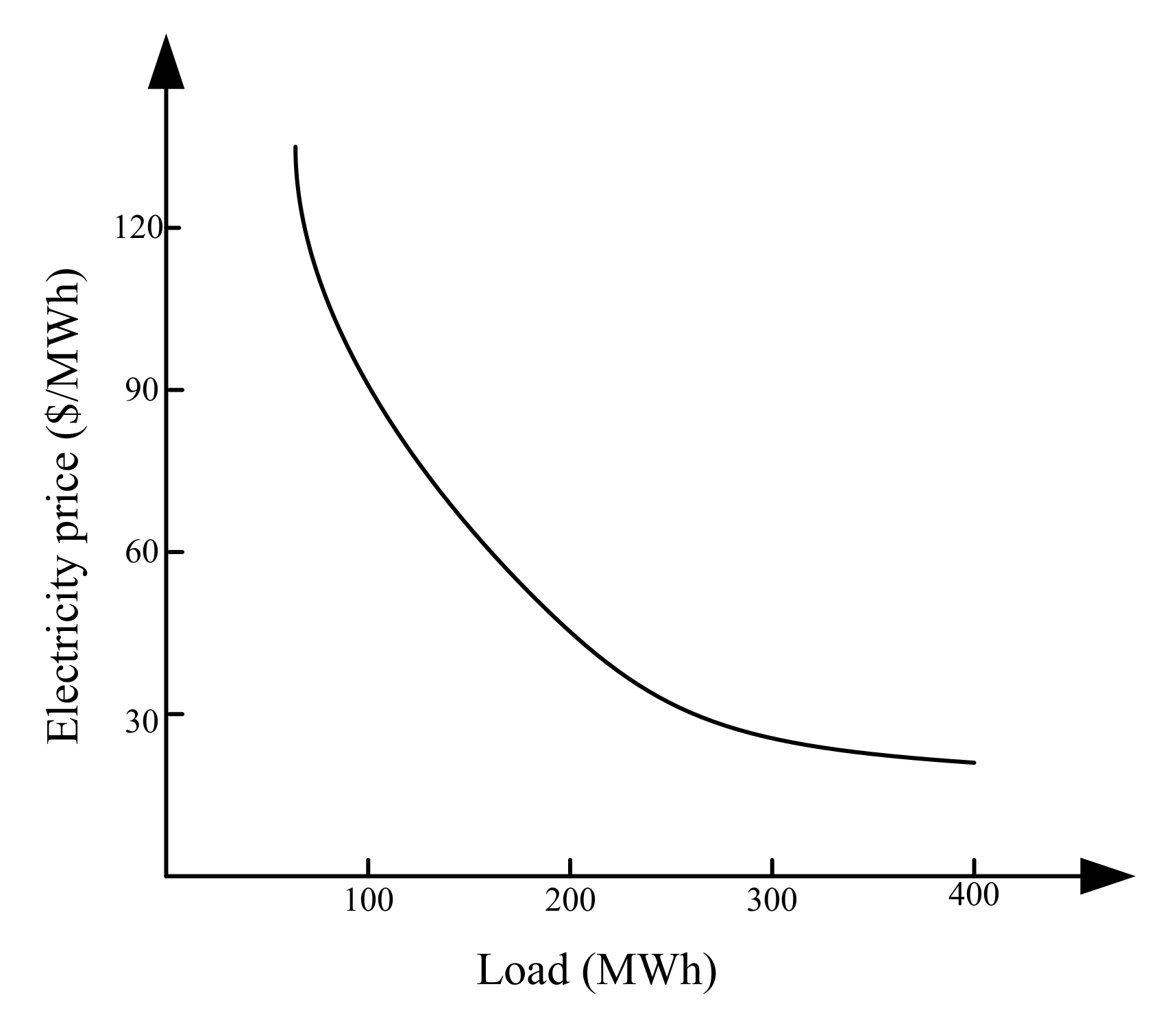
From an economic perspective, the load is closely related to electricity price. Therefore, under the base of meeting the most basic load, users adjust the load demand depending on the TOU electricity price to minimize their electricity cost [19]. In addition to the basic load demand of the user’s life and work, the user may adjust the daily load curve according to the electricity price. For example, users may charge electric vehicles, increase the charging time at the lower electricity price period, and reduce the charging time at the higher electricity price period.
The correlation between the electricity price and load demand is shown in Figure 1. The demand for user load decreases as the electricity price increases, as illustrated in Figure 1. Four different representations of load demand against electricity price were proposed—linear, potential, logarithmic, and exponential representation functions—in [20]. The price elasticity of a load with a linear function was applied herein to optimize the TOU electricity price.
The price elasticity of the load is defined as the sensitive response of the load to the electricity price [19]. The price elasticity of demand is calculated as follows:
where is the initial load demand at time t, and P0(t) is the initial electricity price at time t.
The linear function for the price elasticity of the load can be illustrated as [20]
where a and b denote the coefficients of the linear function of the load demand against the electricity price.
On the basis of Equations (1) and (2), the price elasticity of load demand can be calculated as follows:
Subsequently, the increased load demand can be expressed as
Therefore, the load demand after modifying electricity price can be expressed as
3. Stochastic Problem
The randomness of PV power, wind power, and load demand may significantly affect the dispatch of power systems. The multi-scenario simulation technology is implemented to select several typical system operation states in the proposed dispatch model by using the uncertainty information of the load demand, PV power, and wind power. The discrete probability distribution set of the load, wind power, and PV power is described as follows [13]:
where DL, Dwind, and DPV are the sets of load, wind power, and PV power, respectively; NL is the number of scenarios of load demand; NPV is the number scenarios of PV power; Nwind is the number scenarios of wind power; is the probability of load demand in the i-th scenario; is the probability of PV power in the i-th scenario; is the probability of wind power in the i-th scenario; ∆L is the base deviation of load demand; ∆PPV is the base deviation of PV power; and ∆ Pwind is the base deviation of wind power.
The probabilities of wind power, load demand, and PV power satisfy the following:
The total set D of scenarios for load demand, PV power, and wind power can be calculated as follows:
4. Problem Formulation
In this study, the utilization rate of renewable energy and the economy are two important indices for power system scheduling. The multi-objective function of the proposed dispatch model includes the profit of the power company and demand users, and the rate of abandoning the output power of wind turbines and PV panels.
The relation between the TOU electricity price and the cost of the power company and demand users is analyzed. However, there is no correlation between TOU electricity price and renewable energy power. The cost of the wind generator and PV generator were disregarded, and the cost of the ESS was also ignored in our study. The hybrid microgrid used herein is only composed of solar power generation, wind power generation, and ESS, excluding traditional energy generation.
4.1. Multi-Objective Dispatch Model
In our work, the multi-objective dispatch model is aimed at determining the optimal TOU electricity price. The multi-objective function established in this section includes the following: (1) maximization of the profit of the power company and the demand users, and (2) minimization of the rate of abandoning the total output power of wind panels and PV turbines.
4.1.1. Maximizing the Profit of Power Company and Demand Users
For the economic dispatch of power systems, the profits of the power company and demand users are both considered herein. However, the profits of the power company and demand users may have less or more of an effect on the optimal TOU electricity price, depending on the case. The profit of the power company comprises the income of selling electricity and the penalty cost of power supply shortage. The profit of demand users is to reduce electricity costs after implementing the optimal TOU electricity price. The profit of the demand users is the electricity cost at the initial electricity price minus the electricity cost at the optimal TOU electricity price.
Therefore, the first function (f1) for the power company’s profit and demand users is expressed as follows:
where Procompany is the profit of the power company, Prouser is the profit of demand users, and α and β are the weight coefficients of the profit of the power company and demand users, respectively. In this study, the relation between them is .
- (1)
- Profit of the power company
For the power company, the profit mainly comprises selling electricity to demand users, the generation cost, and the penalty cost for the power supply shortage. In our study, the renewable generation cost was not considered. Therefore, in this study, the profit of the power company includes the penalty cost of power supply shortage and the income of selling electricity to demand users, expressed as
where Pgen(t) is the output power of renewable energy at time t; Pdis(t) is the discharge power of the ESS at time t; u1(t) and u2(t) are binary numbers: u1(t) = 0 and u2(t) = 1 indicates that the load demand exceeds the total renewable energy power at time t; u1(t) = 1 and u2(t) = 0 indicates that the renewable energy power exceeds the load demand at time t; is the penalty coefficient of power supply shortage; and dshort(t) is the shortage of power supply at time t.
- (2)
- Profit of the demand users
For demand users, electricity cost is the first consideration. However, the electricity cost of demand users is mainly affected by the electricity price and load demand. In this study, the profit of the demand users is given by reducing electricity costs after implementing the optimal TOU electricity price. This can be expressed as follows:
where C0 denotes the electricity cost of demand users with the initial electricity price, and CTOU is the electricity cost of demand users with TOU electricity price.
4.1.2. Minimizing the Rate of Abandoning PV Power and Wind Power
Owing to the uncontrollable characteristic of the renewable energy power, when the sum output power of renewable energy exceeds the load demand, the extra output power of wind turbines and PV panels will be abandoned. By optimizing the TOU electricity price, the load curve comes close to the renewable energy power to reduce the rate of abandoning PV power and wind power. The second objective is expressed as follows:
where Pchar(t) is the charge power of the ESS at time t; and PPV.upper(t) and Pwind.upper(t) are the upper PV power and the upper wind power at time t, respectively.
4.2. Constraints
The multi-objective dispatch model proposed herein meets the following equality and inequality constraints (14)–(21).
4.2.1. Power Balance Constraint
For power system scheduling, the output power, charge power, and discharge power of the ESS should be equal to the power supply and charge power of the ESS, which can be expressed as
4.2.2. PV Power and Wind Power Constraints
The wind power and PV power utilized in the hybrid microgrid were mainly determined by the maximum and minimum values of the output power. The utilization of PV power and wind power should satisfy the following constraints:
4.2.3. ESS Constraint
When the ESS is operated during the charging process, battery banks are charged with renewable energy power. The stored energy of the battery is determined by the charge power and stored energy of the previous hour. It is calculated as [21]:
where E(t) is the stored energy of the battery at time t and is the battery charge efficiency.
When the ESS is operated during the discharging process, the battery banks discharge power to load demand. The stored energy of the battery is determined by the discharge power and stored energy of the previous hour. It can be calculated as [21]:
where is the battery discharge efficiency.
Herein, the self-discharge of the ESS is negligible in our work. The state of charge (SOC) constraint is expressed as [22]:
where SOC(t) is the SOC of the ESS at time t, SOC.lower is the lower SOC of the ESS, and SOC.upper is the upper SOC of the ESS.
The constraint of the discharged power for the ESS is expressed as
The constraint of the charging power for the ESS is expressed as
where Pchar.upper and Pdis.upper are the upper charging power and discharged power of the battery banks, respectively, and EESS is the rated capacity of the battery banks.
4.2.4. Optimization Variables
In the multi-objective dispatch model proposed herein, the TOU electricity price is the optimization variable. According to the hourly load data, the hours of one day were divided into three parts: peak period, off-peak period, and valley period. The initial electricity prices were all set to 75 USD/MWh. The three periods in the TOU electricity prices are listed in Table 1. In the electricity market of power systems, to maintain the stability of the electricity price, the electricity price of the power company should be adjusted within a fixed range. The constraints of the TOU electricity price are limited, as shown in Table 2.
5. Multi-Objective Algorithm
The multi-objective genetic algorithm (GA) [23] and particle swarm optimization (MOPSO) [24], as mature optimization algorithms, have been applied by many scholars. In our work, the optimal solution of the multi-objective dispatch mode is determined using MOPSO. A satisfactory solution is selected from the Pareto optimal solution set [25]. The standardized objective function for each solution is expressed as [26]:
where s(x) = [, ] is the standardized objective function of the objective function f = [f1, f2]; f1.max and f2.max are the maxima of the objective functions f1 and f2, respectively; f1.min and f2.min are the minimum values of the objective functions f1 and f2, respectively.
The normalized function value of the nondominated solution can be calculated as [26]:
where is the normalized function value with i nondominated solution, N is the number of objective functions, and M is the number of nondominated solutions. The maximum value of determines the optimal solutions of the multi-objective function.
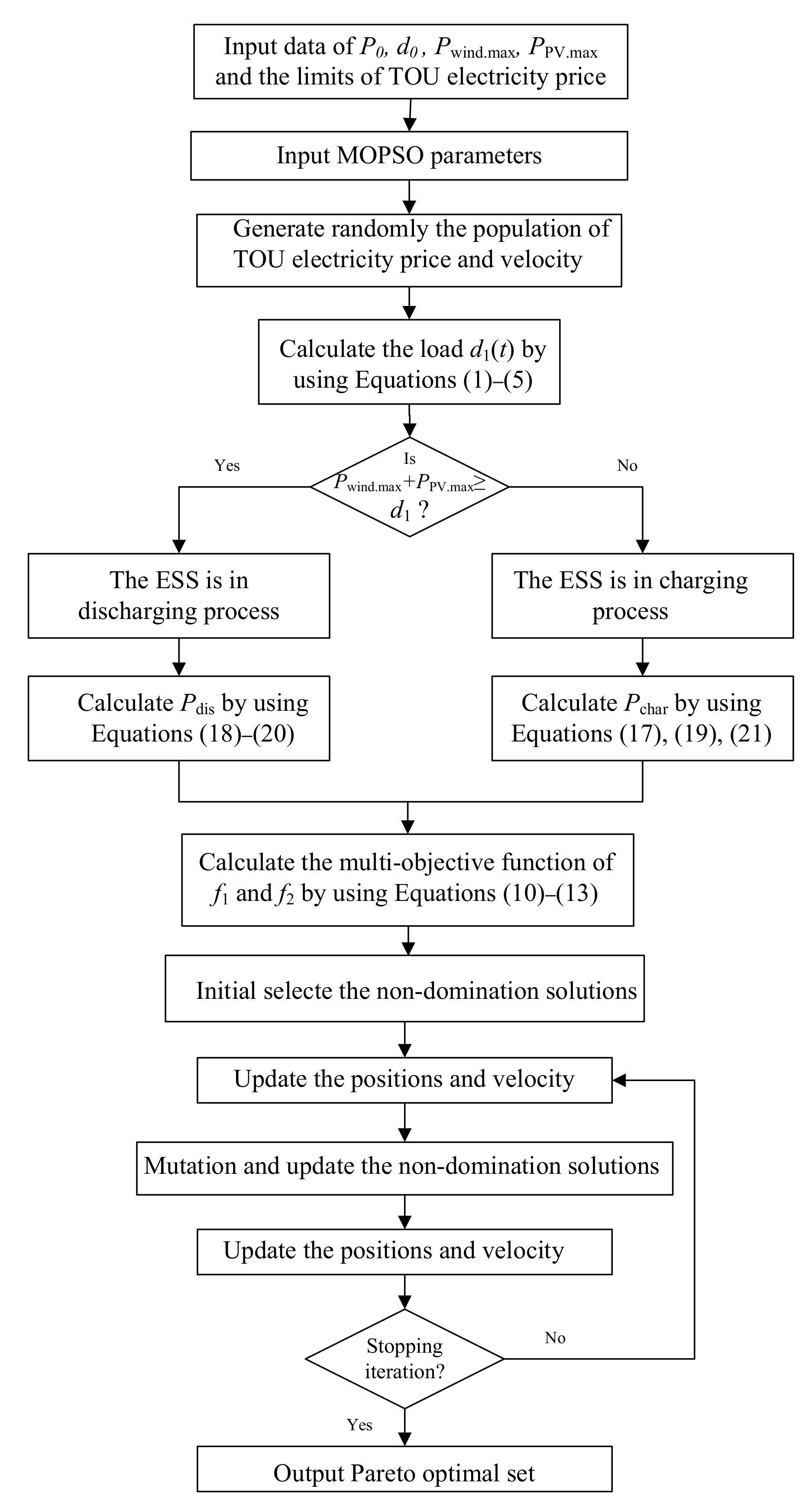
The flowchart shown in Figure 2 presents the step procedure for the multi-objective dispatch model.
- (1)
- The initial data of the load demand, electricity price, wind power, and PV power are input.
- (2)
- The populations of the variables (TOU electricity price) are randomly generated within the limits of TOU electricity price.
- (3)
- The loads that carry out the random TOU electricity price are calculated by Equations (1)–(5).
- (4)
- The load demand and output power of renewable energy are compared to determine the charging or discharging processes of the ESS. If the output power of renewable energy can satisfy the load demand, the ESS is operated during the charging process. If the output power of renewable energy cannot satisfy the load demand, then the ESS is operated during the discharging process. The multi-objective functions of f1 and f2 are calculated using Equations (10)–(13).
- (5)
- The non-domination solution set is obtained from Step (4).
- (6)
- Update the TOU electricity price and velocity.
- (7)
- Update the new solutions by mutating the solutions of Step (6) and determining the new non-domination solution.
- (8)
- Stop criterion. When the number of iterations is less than the number parameters set herein, go to Step (6); otherwise, stop criterion.
- (9)
- The Pareto optimal set was obtained by applying multi-objective particle swarm optimization.
- (10)
- The satisfactory solution is obtained by Equations (22) and (23).
6. Case Study
In this section, a hybrid microgrid composed of PV power plants, wind power plants, and ESSs is used to test the multi-objective dispatch model proposed herein. The ESS parameters are presented in Table 3. The coefficients of the linear function for the price elasticity of load demand a and b are 300 and −1.5, respectively, extracted from [20] with some modifications. The penalty coefficient of the power supply shortage was 70 USD/MWh.
The proposed multi-objective dispatch model was solved using MOPSO in this section. In our MOPSO work, the population size was 20, the number of iterations was 100, and the repository size was 100. The proposed algorithm was implemented in the software package MATLAB 2015 on a PC with an M1 CPU and 8 GB of RAM.
In our work, the number scenarios of load demand, wind power, and PV power were set to 5. We assume that the deviations of wind power, PV power, and load demand obey the standard normal distribution. The base deviation of the load demand, output power of the wind, and PV panels is 15% of the load demand, and the output power of the wind and PV panels. The discrete probability of the output power of the wind and PV panels and the load demand are shown in Table 4, which is from [13] with some modifications. The total number of scenarios was 5 × 5 × 5 = 125. The hourly wind power, PV power, and load demand data for one day are shown in Table 5.
Subsequently, Equation (6) can be expressed as
Five cases were simulated by applying MOPSO to verify the multi-objective dispatch model proposed herein. These five cases were proposed with different profit coefficients. The optimization results were analyzed and compared. The simulation results for these five cases are listed in Table 6 and Table 7. Table 6 illustrates the optimal TOU electricity price, multi-objective function, and profit of the power company and demand users. Table 7 illustrates the proportion of load demand at the three-part period for these five cases.
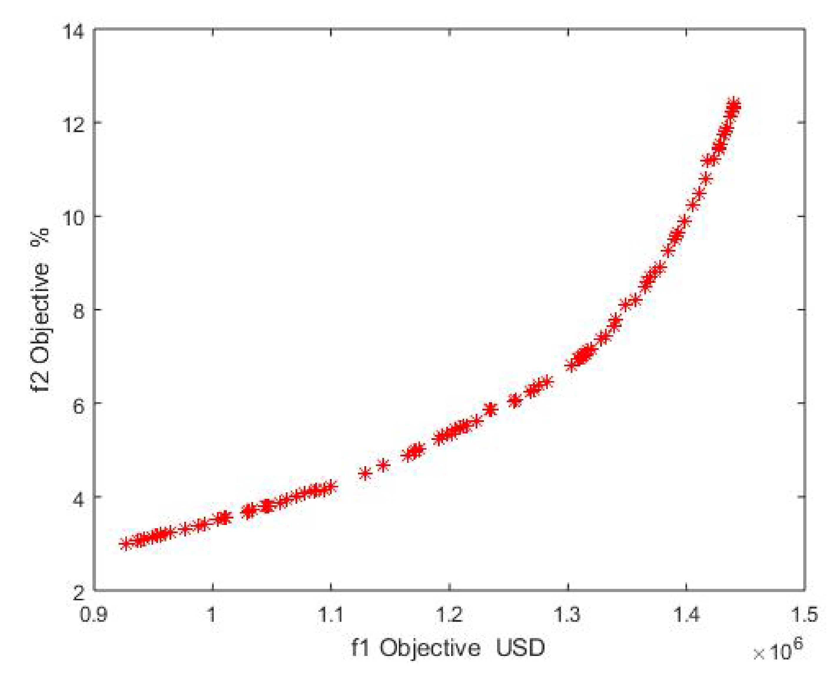
Figure 3 shows the simulation results for the multi-objective dispatch model solved by MOPSO. The profit of the power company and demand users, and the rate of abandoning PV power and wind power, may conflict.
6.1. Base Case
To analyze the economic and the rate of abandoning PV power and wind power, the base case was set to an initial electricity price of 75 USD/MWh in the hybrid microgrid. The proportion of the load in the base case is shown in the first row of Table 6. The multi-objective function of f2 was 6.82%. The profit of the power company and demand users cannot be calculated as the weight coefficients of the power company’s profit and demand users are not set in this case. The proportions of demand load at peak, off-peak, and valley periods were 31.2%, 42.8%, and 26%, respectively.
6.2. Analysis of the Profit of the Power Company and Demand Users
For the profit of demand users, minimizing the electricity price is the optimal solution, as it can obtain the minimum electricity cost of demand users. The weight coefficients of the profit of demand users are higher than those of the power company in Cases 1 and 2. Therefore, in the two cases, the optimal electricity prices of the valley and off-peak periods are 15 USD/MWh and 60 USD/MWh, respectively, which are the lower limits of the TOU electricity price. For Cases 1–3, the weight coefficients of the profit of demand users are progressively reduced. In Cases 1–3, the optimal electricity prices at the peak period are 110 USD/MWh, 114 USD/MWh, and 153 USD/MWh, respectively. In Cases 4 and 5, the weight coefficients of the power company are higher than those of demand users. From the simulation results in Cases 4 and 5, the profits for demand users are −14,109.5 USD and −78,477.3 USD, respectively. Therefore, the profit of the power company increases, and the profit of users is less than zero.
For the profit of the power company, maximizing the electricity price is the optimal solution that can maximize the income of selling electricity for the power company. As shown in Table 5, the off-peak electricity prices of Cases 4 and 5 are 88.7 USD/MWh and 85.4 USD/MWh, respectively. The electricity prices are close to the upper limit of the off-peak electricity price. The valley electricity prices of Cases 4 and 5 are 37.9 USD/MWh and 51.2 USD/MWh, respectively, obviously exceeding those of Case 1 and Case 2. The weight coefficients of the profit of the power company exceed those of demand users in Cases 3 and 4.
In Case 3, the weight coefficients of the profit of demand users and the power company are equal to 0.5. Compared with the results of Cases 1 and 2, the off-peak electricity price is increased by 2.6 USD/MWh as the weight coefficient of the profit of the power company in Case 3 exceeds that in Cases 1 and 2. Moreover, the electricity prices of the valley and off-peak periods in Case 3 are smaller than those in Cases 4 and 5 as the weight coefficient of the profit of users in Case 3 exceeds that in Cases 4 and 5.
6.3. Analysis of the Rate of Abandoning Output Power of Renewable Energy
To minimize the rate of abandoning the output power of renewable energy, the excess output power of renewable energy should be minimized. The hours of exceeding the total output power of renewable energy may occur during the valley period. The sum of the output power of the renewable energy exceeds the load demand.
As shown in Table 6, compared with the base case data, the valley period loads in Cases 1, 2, and 3 are all increased by 2120 MW as the valley electricity price in these three cases was 15 USD/MWh. The valley electricity prices in Cases 4 and 5 are 37.9 USD/MWh and 51.2 USD/MWh, respectively, which are higher than those of the three cases. Therefore, the loads at the valley period in Cases 4 and 5 only increased by 1312 MW and 841 MW, respectively. During the valley period, the loads in Cases 4 and 5 were less than those in the three cases.
From the above simulation results, the weight coefficients of the profit of demand users gradually decrease. The weight coefficients of the profit of the power company gradually increase from the results of Cases 1–5. With the increasing weight coefficients of the power company profit, the electricity price and the rate of abandoning PV power and wind power increased.
The load demand of the valley period increases, and the load demand of the peak period is reduced. The results of the first three cases were similar. This is as the TOU electricity prices of these three cases are close to the lower limit of the electricity price. The TOU electricity price in Case 3 was the upper limit of the electricity price.
7. Conclusions
DR plays a significant role in power system scheduling. As one of the methods for the DR, the price elasticity of load demands was applied herein to establish a multi-objective dispatch model for integration to minimize the rate of abandoning renewable energy generation power and maximize the profit of the power company and demand users. The hybrid microgrid comprises renewable generation and an ESS. The uncertainty problem of renewable generation is considered in this study. MOPSO was applied to obtain the solutions for the optimal TOU electricity price for the proposed multi-objective model.
The simulation results of five cases with different profit weight coefficients were analyzed and compared to prove the feasibility of the proposed multi-objective dispatch model. The results listed in Table 6 show that, with the increasing weight coefficients of the power company profit, electricity price, and the rate of abandoning PV power and wind power are increased. The results in Figure 3 show that with an increase in the profit of the power company and demand users, the rate of abandoning PV power and wind power correspondingly decrease. We can draw the conclusion that the profits of power companies and demand users, and the rate of abandoning PV power and wind power, are conflicting. With an increase in the profit weight coefficient, the optimal electricity price increases. Simultaneously, the rate of abandoning PV power and wind power increased. In our work, the elastic price of the load demand with a linear function is employed to optimize the TOU electricity price. However, the coefficients of the linear function for the price elasticity of load demand should be more accurate, which could form the basis for the next research topic.
Author Contributions
Conceptualization, N.-C.Y.; Data curation, N.Z.; Formal analysis, N.Z.; Funding acquisition, N.-C.Y.; Investigation, N.Z.; Methodology, N.Z. and N.-C.Y.; Resources, N.-C.Y.; Software, N.Z.; Supervision, N.-C.Y. and J.-H.L.; Validation, N.Z.; Visualization, N.-C.Y.; Writing—original draft, N.Z.; Writing—review & editing, N.-C.Y. All authors have read and agreed to the published version of the manuscript.
Funding
This work was partially supported by the Ministry of Science and Technology (MOST) in Taiwan (MOST 109-3111-8-011-001) and Delta–NTUST Joint Research Center.
Acknowledgments
This work was partially supported by the Ministry of Science and Technology (MOST) in Taiwan. The authors would like to thank the funding provided by MOST (MOST 109-3111-8-011-001) and DELTA-NTUST Joint Research Center.
Conflicts of Interest
The authors declare no conflict of interest.
References
- Zong, W.G. Size optimization for a hybrid photovoltaic–wind energy system. Int. J. Electr. Power Energy Syst. 2012, 42, 448–451. [Google Scholar]
- Parvania, M.; Fotuhi-Firuzabad, M. Integrating Load Reduction Into Wholesale Energy Market With Application to Wind Power Integration. IEEE Syst. J. 2012, 6, 35–45. [Google Scholar] [CrossRef]
- Liu, J.; Fang, W.; Zhang, X.; Yang, C. An Improved Photovoltaic Power Forecasting Model With the Assistance of Aerosol Index Data. IEEE Trans. Sustain. Energy 2015, 6, 1–9. [Google Scholar] [CrossRef]
- Kapsali, M.; Kaldellis, J.K. Combining hydro and variable wind power generation by means of pumped-storage under economically viable terms. Appl. Energy 2010, 87, 3475–3485. [Google Scholar] [CrossRef]
- Bayer, P.; Rybach, L.; Blum, P.; Brauchler, R. Review on life cycle environmental effects of geothermal power generation. Renew. Sustain. Energy Rev. 2013, 26, 446–463. [Google Scholar] [CrossRef]
- Parastegari, M.; Hooshmand, R.A.; Khodabakhshian, A.; Zare, A.H. Joint operation of wind farm, photovoltaic, pump-storage and energy storage devices in energy and reserve markets. Int. J. Electr. Power Energy Syst. 2015, 64, 275–284. [Google Scholar] [CrossRef]
- Zhao, H.; Wu, Q.; Hu, S.; Xu, H.; Rasmussen, C.N. Review of energy storage system for wind power integration support. Appl. Energy 2015, 137, 545–553. [Google Scholar] [CrossRef]
- Abdi, H.; Dehnavi, E.; Mohammadi, F. Dynamic Economic Dispatch Problem Integrated With Demand Response (DEDDR) Considering Non-Linear Responsive Load Models. IEEE Trans. Smart Grid 2016, 7, 2586–2595. [Google Scholar] [CrossRef]
- Aghaei, J.; Alizadeh, M.I. Critical peak pricing with load control demand response program in unit commitment problem. IET Gener. Transm. Distrib. 2013, 7, 681–690. [Google Scholar] [CrossRef]
- Qian, L.P.; Zhang, Y.; Huang, J.; Wu, Y. Demand Response Management via Real-Time Electricity Price Control in Smart Grids. IEEE J. Sel. Areas Commun. 2013, 31, 1268–1280. [Google Scholar] [CrossRef]
- Asadinejad, A.; Tomsovic, K. Optimal Operation for Economic and Exergetic Objectives of a Multiple Energy Carrier System Considering Demand Response Program. Energies 2019, 12, 3995. [Google Scholar] [CrossRef] [Green Version]
- Parvania, M.; Fotuhi-Firuzabad, M.; Shahidehpour, M. Optimal Demand Response Aggregation in Wholesale Electricity Markets. IEEE Trans. Smart Grid 2013, 4, 1957–1965. [Google Scholar] [CrossRef]
- Nojavan, S.; Zare, K.; Mohammadi-Ivatloo, B. Optimal stochastic energy management of retailer based on selling price determination under smart grid environment in the presence of demand response program. Appl. Energy 2017, 187, 449–464. [Google Scholar] [CrossRef]
- Yu, R.; Yang, W.; Rahardja, S. A Statistical Demand-Price Model With Its Application in Optimal Real-Time Price. IEEE Trans. Smart Grid 2012, 3, 1734–1742. [Google Scholar] [CrossRef]
- Nojavan, S.; Mohammadi-Ivatloo, B.; Zare, K. Optimal bidding strategy of electricity retailers using robust optimisation approach considering time-of-use rate demand response programs under market price uncertainties. Gener. Transm. Distrib. IET 2015, 9, 328–338. [Google Scholar] [CrossRef]
- Hu, F.; Feng, X.; Cao, H. A Short-Term Decision Model for Electricity Retailers: Electricity Procurement and Time-of-Use Pricing. Energies 2018, 11, 3258. [Google Scholar] [CrossRef] [Green Version]
- Haider, H.T.; See, O.H.; Elmenreich, W. Residential demand response scheme based on adaptive consumption level pricing. Energy 2016, 113, 301–308. [Google Scholar] [CrossRef]
- Wu, Z.; Tazvinga, H.; Xia, X. Demand side management of photovoltaic-battery hybrid system. Appl. Energy 2015, 148, 294–304. [Google Scholar] [CrossRef] [Green Version]
- Aalami, H.A.; Moghaddam, M.P.; Yousefi, G.R. Modeling and prioritizing demand response programs in power markets. Electr. Power Syst. Res. 2010, 80, 426–435. [Google Scholar] [CrossRef]
- Yousefi, S.; Moghaddam, M.P.; Majd, V.J. Optimal real time pricing in an agent-based retail market using a comprehensive demand response model. Energy 2011, 36, 5716–5727. [Google Scholar] [CrossRef]
- Zhang, Y.; Wang, J.; Berizzi, A.; Cao, X. Life cycle planning of battery energy storage system in off-grid wind–solar–diesel microgrid. IET Gener. Transm. Distrib. 2018, 12, 4451–4461. [Google Scholar] [CrossRef]
- Tazvinga, H.; Xia, X.; Zhang, J. Minimum cost solution of photovoltaic–diesel–battery hybrid power systems for remote consumers. Sol. Energy 2013, 96, 292–299. [Google Scholar] [CrossRef]
- Yang, H.; Wei, Z.; Lin, L.; Fang, Z. Optimal sizing method for stand-alone hybrid solar–wind system with LPSP technology by using genetic algorithm. Sol. Energy 2008, 82, 354–367. [Google Scholar] [CrossRef]
- Borhanazad, H.; Mekhilef, S.; Ganapathy, V.G.; Modiri-Delshad, M.; Mirtaheri, A. Optimization of micro-grid system using MOPSO. Renew. Energy 2014, 71, 295–306. [Google Scholar] [CrossRef]
- Lokeshgupta, B.; Sivasubramani, S. Multi-objective dynamic economic and emission dispatch with demand side management. Int. J. Electr. Power Energy Syst. 2018, 97, 334–343. [Google Scholar] [CrossRef]
- Sedighizadeh, M.; Esmaili, M.; Jamshidi, A.; Ghaderi, M.-H. Stochastic multi-objective economic-environmental energy and reserve scheduling of microgrids considering battery energy storage system. Int. J. Electr. Power Energy Syst. 2019, 106, 1–16. [Google Scholar] [CrossRef]
Figure 1.
Electricity price against load demand.

Figure 2.
Flowchart of the optimization calculation.

Figure 3.
MOPSO simulation results for the multi-objective dispatch model.


Table 1.
Three periods in the TOU electricity price.
| Time (h) | Initial Electricity Price (USD/MWh) | |
|---|---|---|
| Off-peak | 7–9, 14–19, 22 | 75 |
| Peak | 10–13, 20–21 | 75 |
| Valley | 1–6, 23–24 | 75 |
Table 2.
Constraint of TOU electricity price.
| Lower Limit (USD/MWh) | Upper Limit (USD/MWh) | |
|---|---|---|
| Peak | 90 | 153 |
| Off-peak | 60 | 90 |
| Valley | 15 | 60 |
Table 3.
Parameters of ESS.
| Parameters | |
|---|---|
| Power capacity (MW) | 1000 |
| 0.9 | |
| 0.1 | |
| 0.1 | |
| 1 | |
| 1 |
Table 4.
Probability of PV power, wind power, and load demand.
| Wind Power | PV Power | Load Demand | Probability |
|---|---|---|---|
| 0.7 | 0.7 | 0.7 L | 0.05 |
| 0.85 | 0.85 | 0.85 L | 0.15 |
| L | 0.5 | ||
| 1.15 | 1.15 | 1.15 L | 0.15 |
| 1.3 | 1.3 | 1.3 L | 0.05 |
Table 5.
Hourly data of PV power, wind power, and load demand in one day.
| Time (h) | 1 | 2 | 3 | 4 | 5 | 6 | 7 | 8 | 9 | 10 | 11 | 12 |
| Load (MW) | 700 | 750 | 850 | 950 | 100 | 1100 | 1150 | 1200 | 1300 | 1400 | 1450 | 1500 |
| PV (MW) | 0 | 0 | 0 | 0 | 0 | 0 | 120 | 180 | 360 | 420 | 550 | 430 |
| Wind (MW) | 1430 | 1300 | 1235 | 1105 | 975 | 910 | 1087 | 1080 | 1005 | 560 | 465 | 620 |
| Time (h) | 13 | 14 | 15 | 16 | 17 | 18 | 19 | 20 | 21 | 22 | 23 | 24 |
| Load (MW) | 1400 | 1300 | 1200 | 1050 | 1000 | 1100 | 1200 | 1400 | 1300 | 1100 | 900 | 800 |
| PV (MW) | 370 | 300 | 255 | 200 | 100 | 0 | 0 | 0 | 0 | 0 | 0 | 0 |
| Wind (MW) | 610 | 1065 | 1005 | 902 | 950 | 1155 | 1260 | 980 | 910 | 1155 | 1170 | 1040 |
Table 6.
Simulation results of five cases.
| α | β | TOU Price (USD/MWh) | Objective Function | Profit of the Power Company and Demand Users | |||||||
|---|---|---|---|---|---|---|---|---|---|---|---|
| Valley | Off-Peak | Peak | f1 (USD) | f2 (%) | Procompany (USD) | Prousers (USD) | Income of Selling Electricity | Penalty Cost of Power Supply Shortage | |||
| Base | × | × | 75.0 | 75.0 | 75.0 | × | 6.82 | 1,692,909.1 | 0 | 1,856,849.5 | 163,940.4 |
| Case 1 | 0.3 | 0.7 | 15.0 | 60.0 | 111.0 | 698,347.0 | 5.33 | 1,287,124.6 | 377,918.7 | 1,471,612.6 | 184,488.0 |
| Case 2 | 0.4 | 0.6 | 15.0 | 60.0 | 140.0 | 792,943.3 | 4.74 | 1,458,766.9 | 349,061.0 | 1,584,055.2 | 125,288.2 |
| Case 3 | 0.5 | 0.5 | 15.0 | 62.6 | 153.0 | 928,014.4 | 5.51 | 1,519,936.6 | 336,092.2 | 1,624,858.3 | 10,4921.7 |
| Case4 | 0.6 | 0.4 | 37.9 | 88.7 | 112.5 | 1,102,424.1 | 6.54 | 1,846,779.9 | −14,109.5 | 1,934,830.9 | 88,051.0 |
| Case 5 | 0.7 | 0.3 | 51.2 | 85.4 | 110.6 | 1,315,901.6 | 7.06 | 1,913,492.7 | −78,477.3 | 1,997,332.4 | 83,839.7 |
Table 7.
Proportion of load demand in each period.
| Load Distribution | ||||||
|---|---|---|---|---|---|---|
| Valley (MW) | Proportion of Valley % | Off-Peak (MW) | Proportion of Off-Peak % | Peak (MW) | Proportion of Peak % | |
| Base case | 7050 | 26.0 | 11,600 | 42.8 | 8450 | 31.2 |
| Case 1 | 9170 | 32.1 | 12,472 | 43.7 | 6925 | 24.2 |
| Case 2 | 9170 | 33.5 | 12,472 | 45.6 | 5696 | 20.8 |
| Case 3 | 9170 | 34.4 | 12,320 | 46.3 | 5146 | 19.3 |
| Case 4 | 8362 | 32.1 | 10,805 | 41.5 | 6863 | 26.4 |
| Case 5 | 7891 | 30.6 | 10,995 | 42.6 | 6941 | 26.9 |
Publisher’s Note: MDPI stays neutral with regard to jurisdictional claims in published maps and institutional affiliations. |
© 2021 by the authors. Licensee MDPI, Basel, Switzerland. This article is an open access article distributed under the terms and conditions of the Creative Commons Attribution (CC BY) license (https://creativecommons.org/licenses/by/4.0/).
Share and Cite
MDPI and ACS Style
Zhang, N.; Yang, N.-C.; Liu, J.-H. Optimal Time-of-Use Electricity Price for a Microgrid System Considering Profit of Power Company and Demand Users. Energies 2021, 14, 6333. https://0-doi-org.brum.beds.ac.uk/10.3390/en14196333
AMA Style
Zhang N, Yang N-C, Liu J-H. Optimal Time-of-Use Electricity Price for a Microgrid System Considering Profit of Power Company and Demand Users. Energies. 2021; 14(19):6333. https://0-doi-org.brum.beds.ac.uk/10.3390/en14196333
Chicago/Turabian StyleZhang, Ning, Nien-Che Yang, and Jian-Hong Liu. 2021. "Optimal Time-of-Use Electricity Price for a Microgrid System Considering Profit of Power Company and Demand Users" Energies 14, no. 19: 6333. https://0-doi-org.brum.beds.ac.uk/10.3390/en14196333
Note that from the first issue of 2016, this journal uses article numbers instead of page numbers. See further details here.