Lifetime Assessment of PILC Cables with Regard to Thermal Aging Based on a Medium Voltage Distribution Network Benchmark and Representative Load Scenarios in the Course of the Expansion of Distributed Energy Resources

Abstract

The decentralized feed-ins from distributed energy resources (DER) represent a significant change in the manner in which the power grid is used. If this leads to high loads on electrical equipment, its aging can be accelerated. This applies in particular with regard to the thermal aging of older generations of power cables, namely paper insulated lead covered (PILC) cables. This type of power cable can still be found frequently in medium voltage (MV) networks. If aging of these cables is significantly accelerated in the presence of DER, distribution system operators (DSO) could face unplanned premature cable failures and a high replacement demand and costs. Therefore, this paper investigates the thermal aging of PILC cables in a MV distribution network benchmark for different load scenarios, using standardized load profiles and representative expansion scenarios for wind power and photovoltaics plants in particularly affected network areas in Germany. A main objective of this paper is to present a methodology for estimating the thermal degradation of PILC cables. An approach is used to draw simplified conclusions from the loading of cables to their conductor or insulation temperature. For this purpose, mainly Joule losses are considered. In addition, thermal time constants are used for the heating and cooling processes. Based on the insulation temperature, thermal aging is determined using the Arrhenius law or the Montsinger rule. However, it is important to note that there is an urgent need for research on reference data in this area. For this reason, the results of the lifetime estimation presented in this paper should only be considered as an approximation if the selected reference data from the literature for the aging model are actually applicable. The lifetime assessment is performed for a highly utilized line segment of the network benchmark. Accordingly, extreme values are examined. Different operational control strategies of DSO to limit cable utilization are investigated. The results show that the expansion of DER can lead to a short but high cable utilization, although the average utilization does not increase or increases only slightly. This can lead to significantly lower cable lifetimes. The possible influence of these temporarily high loads is shown by comparing the resulting cable lifetime with previous situations without DER. It is also shown that DSO could already reduce excessive aging of PILC cables by preventing overloads in a few hours of a year. In addition to these specific results, general findings on the network load due to the influence of DER are obtained, which are of interest for congestion management.

1. Introduction

In order to limit climate change, a transition of the energy system to generation technologies without direct emissions of greenhouse gases is a basic prerequisite. Key technologies in this respect are wind power and photovoltaic (PV) plants. These distributed energy resources (DER) are characterized by fluctuating power generation due to their dependence on the natural availability of solar radiation and wind. Furthermore, these plants are primarily connected to the distribution grid due to their power size. The decentralized feed-ins of DER represent a significant change in the manner in which the power grid is used. In the past, the usage of the grid was structured top-down, with feed-ins at high voltage levels and loads at lower voltage levels. In sum, the expansion of DER leads to a change in the utilization of the power grid—especially of the distribution network. Distribution system operators (DSO) have to adapt the correlating new challenges. One challenge is that a changing load behavior of distribution networks in turn influences the aging of electrical equipment. For example, the aging of cables is dependent on their load. Medium voltage (MV) networks are particularly affected, as a relatively high proportion of rather outdated cables are installed. Further aging has a significant impact on the number of failures in the near future. As grid renewal is limited for economic reasons and due to capacity constraints of DSO, operational control measures to limit the utilization of electrical equipment should be considered, taking into account the remaining service life. In the past, estimates of the remaining lifetime of electrical equipment were based on relatively even, low, and predictable utilization rates. PV and wind power plants have highly volatile feed-in profiles. The expansion of these technologies in distribution grids can lead to short but high peak loads for electrical equipment as well as a higher overall utilization, which influences the aging behavior. The lifetime assessment of grid assets is complex, as DSO on the one hand often lack knowledge about the utilization and the remaining lifetime of individual electrical equipment. On the other hand, suitable models for estimating the aging with regard to variable stresses are necessary [1].

This paper describes the thermal aging of paper insulated lead covered (PILC) cables. This type of power cable can be found frequently in MV networks, even if this type was mainly replaced by cross-linked polyethylene (XLPE) cables for new installations since the 1970s. In 1997, PILC cables represented around 50% of the cable line length of the MV grid in Germany. In 2019, the majority of these cables were older than 40 years [2]. In 2005, screened and belted PILC (36% and 22%) and XLPE (33%) cables were the most commonly used MV cable types worldwide [3].

This paper starts with a general description of stresses on cables (see Section 2). In this context, thermal stress is the main focus of interest. The Arrhenius law or Montsinger rule are used to describe the degeneration based on thermal stress (see Section 3). To investigate the influence of DER to the grid, a simulation of a network benchmark is executed. Various load scenarios are considered for the network benchmark, using standardized load profiles and representative expansion scenarios for wind power and PV plants in particularly affected MV network areas in Germany (see Section 4 and Section 5). The aging behavior for the different load scenarios is not presented for the entire network benchmark. Instead, a lifetime assessment for a highly utilized line segment is shown. Accordingly, extreme values are examined. The main objective of this paper is to provide a methodology for estimating the thermal degradation of PILC cables and to show the potential influence of temporarily high loads. To this end, thermal aging of cables in the course of the integration of DER into the grid is compared with previous situations without DER (see Section 6).

2. Thermal Stress

Electrical equipment is exposed to electrical, thermal and mechanical stresses. This can be caused by external influences, such as solar radiation, external heat sources, lightning discharges, neighbouring conductors, wind, and ice loads. Stresses are also induced by internal influences such as electric field intensity, Joule losses, dielectric and magnetic losses, magnetic forces, thermal expansion forces and vibrations. In addition, atmospheric stresses can also occur due to chemical influences and pollution. Depending on the duration of exposure, a distinction can be made between long-term and short-term stresses. Continuous as well as short-term loads place thermal and mechanical stress on electrical equipment, which has an influence on their insulation properties and aging [4]. For the oil-impregnated insulation of PILC cables thermal degradation is the main aging mechanism, therefore, only this is considered in the following [1].

2.1. Heat Sources

Internal heat sources for cables are Joule losses as well as hysteresis, eddy-current and dielectric losses. Additional thermal stress is caused by external heat sources such as other cables or supply lines in the vicinity [4,5]. Joule losses $P_{Loss}$ are load-dependent, caused by resistances $R$ and the apparent currents ${\underset{\_}{I}}_a$:

$$\begin{gathered} P_{Loss}={\left|{\underset{\_}{I}}_a\right|}^2·R_{DC}·k_c \\ \mathrm{with}: \\ R=R_{{\vartheta }_R}·\left[1+\alpha ·\left({\vartheta }_n-{\vartheta }_R\right)\right] \end{gathered}$$

(1)

where $R_{{\vartheta }_R}$ is the resistance for a reference temperature—in most cases 20 °C ($R_{20}$), since this corresponds to the average ambient temperature in regions under consideration [4]—and $\alpha$ is the material specific temperature coefficient, which indicates a linear resistance change as a function of temperature (${\alpha }_{Cu}=3.85\times {10}^{-3}$). There may be a significant increase in resistance due to the skin and proximity effect. Because of these current displacement effects, the AC resistance of a conductor is greater than its DC resistance $R_{DC}$ by a current displacement factor $k_c$. This increase should to be taken into account for conductor cross-sections larger than 185 mm² [6]. Eddy-current and hysteresis losses of cables can be considered as a function of the Joule losses via loss factors [6,7]. Dielectric losses are negligible for low voltages, e.g., this is recommended for voltages below 44 kV in the National Electrical Code (USA) [8]. Following the previous explanations, the internal heat sources of MV cables can be limited to Joule losses and losses converted to them.

2.2. Permissible Amapcity

The maximum permissible current of cables is specified in standards [9,10]. Manufacturers also provide information and recommendations for current-carrying capacities under different conditions [11]. The basis for the first international standard IEC 60287 was the formula system developed by J.H. Neher and M.H. McGrath in 1957 [8]. This standard only covers the steady-state at continuous load. Transient and cyclic loads are to be calculated according to IEC 60853 [12]. In Germany, also DIN VDE 0276 for power distribution cables has to be considered. The standards allow a comparable calculation of the load capacity of cables systems, verified by measurements. The methodology in the standards is built on analytical approximation formulas, which are often conservative. These are based on a thermal equivalent circuit diagram with heat sources and thermal resistors (cf. [13,14]). Today, numerical methods can be used for more accurate calculations, e.g., the finite element method (FEM, see IEC TR 62095). The normative specifications in DIN VDE 0276 are the result of calculations, tests and many years of experience. The rated values are based on boundary conditions that are usually found in Central Europe, such as ambient conditions of 30 °C air temperature and 20 °C ground temperature. In addition, a daily load factor of 0.7 is generally assumed for underground cables. This relies on a load profile that is common for DSO. For overhead lines and cables installed in the air, a continuous load, i.e., a load factor of 1.0, is taken into account, since their thermal time constants are relatively short compared to underground cables [15].

To consider the operating and ambient conditions as well as the type of installation, a permissible current $I_p$, which deviates from the rated current $I_r$, must be determined using conversion factors $\prod f$ [10,15,16]:

$$I_p=I_r·\prod f$$

(2)

If the maximum allowable temperatures are maintained, cables can also be operated in cyclical operation, e.g., at a daily load factor of 0.7, above their rated current. Depending on the preload and the overload duration, a potential overload can be determined without exceeding certain temperatures [11,15,16]. In practice, DSO often assume that short-term and infrequent cable overloads of up to 20% are acceptable [11,17].

In Section 6, a lifetime assessment is presented for the cable type NEKEBA 3 × 120 mm² 12/20 KV (U_max = 24 kV). Corresponding data are given in

Table 1. Data for cable type NEKEBA 3 × 120 mm² 12/20 kV (U_max = 24 kV) [18].

Rated current per conductor	Ir	302 A
Direct current resistance at 65 °C per conductor	RDC	0.18 Ω/km
Active resistance at 65 °C per conductor	RAC	0.184 Ω/km
Joule losses per cable based on active resistance	Ploss	50.3 kW/km

.

Factors for the conversion of the rated current into the permissible current are shown in

Table 2. Conversion factors from [18] and typical seasonal ground temperatures in Central Europe from [12,15,19].

Maximum Allowable Temperature of 65 °C, Installation in Ground and Load Factor of 1.0		f1 ∙ f2 = ∏f
Ground Temperature	Specific Ground Resistance
20 °C (Typical for July, August, September)	1 km/W	$0.90\times 0.91=0.82$
	2.5 km/W	$0.74\times 0.91=0.67$
15 °C (Typical for May, June, October)	1 km/W	$0.94\times 0.91=0.86$
	2.5 km/W	$0.78\times 0.91=0.71$
10 °C (Typical for March, April, November)	1 km/W	$0.97\times 0.91=0.88$
	2.5 km/W	$0.82\times 0.91=0.75$
5 °C (Typical for December, January, February)	1 km/W	$1.00\times 0.91=0.91$
	2.5 km/W	$0.85\times 0.91=0.77$

. The rated values are based on a load factor of 0.7, a ground temperature of 20 °C and a specific ground resistance of 1 km/W. The conversion factors from the table show that for soils with a resistivity of 2.5 km/W instead of 1 km/W the permissible current is lower by a factor between 0.82 and 0.85 to maintain the maximum allowable temperature. Furthermore, for every 5 °C lower soil temperature, the acceptable current is higher by a factor between 1.03 and 1.054.

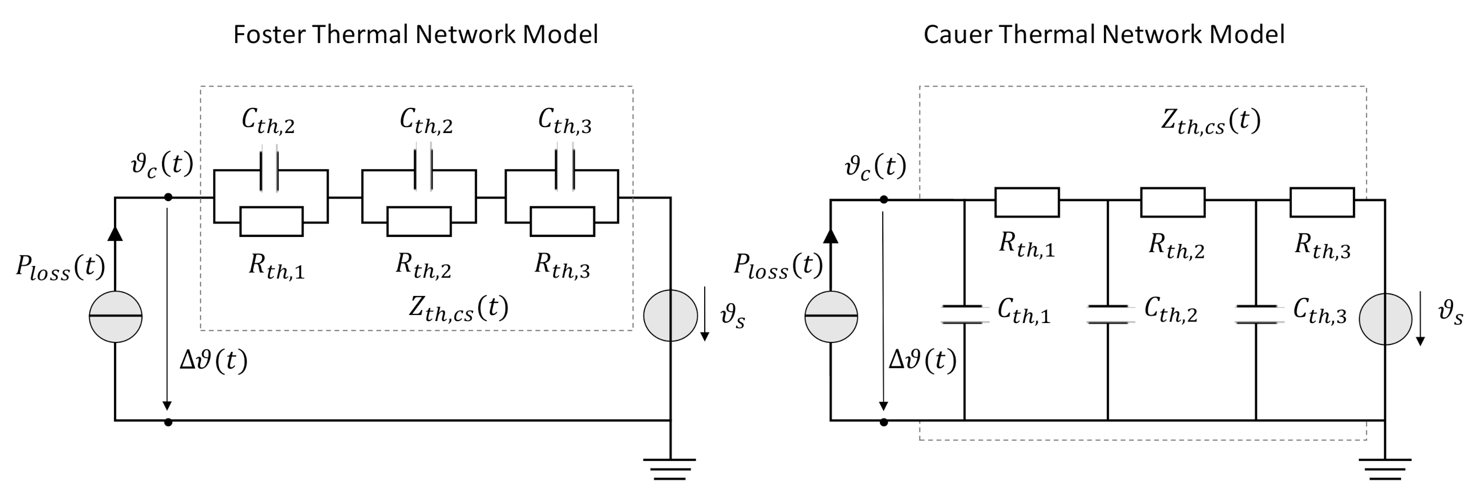
2.3. Thermal Analysis

The heating of a medium is determined by the amount of internal and external heat sources as well as by heat storage and release. The energy balance of supplied, stored and transferred heat according to first law of thermodynamics is the basis for thermal analysis. Heat transfer is caused due to temperature differences. The direction of heat transfer is always from a location with higher temperature to a location with lower temperature. The heat transfer can take place by heat conduction, convection or radiation [5]. A possibility of thermal analysis is the so-called thermal network method. This method is based on the analogy between variables and constants of the thermal and electrical field, summarized in

Table 3. Analogy between variables and constants of the thermal and electrical field [4,5].

Electrical Field			Thermal Field
Parameter	Formula Symbol	Unit	Parameter	Formula Symbol	Unit
Potential difference	U	(V)	Temperature difference	Δ $\vartheta$	(K)
Electric current	I	(A)	Heat flow	Pth	(W)
Electrical resistance	R	(Ω)	Thermal resistance	Rth	(K/W)
Electrical capacity	C	(As/V)	Thermal capacity	Cth	(Ws/K)
Electrical energy	W	(Ws)	Heat	Qth	(Ws)

. Accordingly, the thermal processes can be described with a thermal network analogous to an electric network [20].

Thermal networks consist of sources and sinks as well as thermal resistances and capacities. If $C_{th}$ is related to the mass of medium $m$, the corresponding specific thermal capacity $c$ is obtained:

$$C_{th}=\frac{\Delta Q}{\Delta \vartheta }=c·m$$

(3)

The thermal capacity indicates how much heat has to be supplied to or removed from a medium to cause a certain temperature change. The thermal resistance of the surrounding environment represents the greatest uncertainty for the thermal analysis of underground power cables. This is due to the fact that conductivity of the ground is highly dependent on parameters such as humidity and temperature, which are subject to local and temporal fluctuations. The thermal resistance of soil can vary between 0.4 and 4 km/W, with typical values between 0.8 and 1.3 km/W [21].

In addition, drying-out of the soil at higher temperatures sets in (cf. [13,14,22,23]). According to IEC 60287 (2005), in stationary observations, drying-out takes place at a critical excess temperature of 15 °C. Above this temperature, a specific soil resistance of 2.5 km/W and below 1.0 km/W is assumed [7].

The energy balance of a cable consists of heat sources, such as Joule losses $Q_{loss}$, the stored heat $Q_{st}$ and the transferred heat $Q_t$ during a differential time period $dt$:

$$\begin{gathered} Q_{loss}=P_{loss}·dt=Q_{st}+Q_t=C_{th}·d\vartheta +\frac{\Delta \vartheta ·dt}{R_{th}} \\ \mathrm{with}: \\ \Delta \vartheta ={\vartheta }_m-{\vartheta }_s \end{gathered}$$

(4)

where $\Delta \vartheta$ is the difference between the medium temperature ${\vartheta }_m$ and the surrounding temperature ${\vartheta }_s$. The first-order differential equation with constant coefficients is as follows [24,25]:

$$\begin{gathered} P_{loss}=C_{th}·\frac{d\vartheta }{dt}+\frac{\Delta \vartheta }{R_{th}} \\ \mathrm{multiplied} \mathrm{by} R_{th} \\ {P}_{loss}·R_{th}=C_{th}·R_{th}·\frac{d\vartheta }{dt}+\Delta \vartheta \end{gathered}$$

(5)

Simplified with constant surrounding temperature ${\vartheta }_S=const.$:

$$\begin{gathered} R_{th}·P_{loss}\left(t\right)=\tau ·\frac{d\left[\Delta \vartheta \left(t\right)\right]}{dt}+\Delta \vartheta \left(t\right) \\ \mathrm{with}: \\ \tau =R_{th}·C_{th} \\ \mathrm{converted}: \\ \Delta \vartheta \left(t\right)=R_{th}·P_{loss}\left(t\right)-\tau ·\frac{d\Delta \vartheta \left(t\right)}{dt} \end{gathered}$$

(6)

where $\tau$ is the thermal time constant. For the time-dependent temperature $\vartheta \left(t\right)$ of the medium results (index $m$ is omitted for clarity):

$$\vartheta \left(t\right)={\vartheta }_0+\Delta \vartheta \left(t\right)={\vartheta }_0+\left({\vartheta }_{\infty }-{\vartheta }_0\right)·\left[1-e^{\left(\frac{-t}{\tau }\right)}\right]$$

(7)

where ${\vartheta }_{\infty }$ is the steady-state temperature and ${\vartheta }_0$ is the initial temperature. The temperature rises until there is a balance between the energy supplied and the energy removed by heat transfer. At this point the stationary or steady-state temperature is reached [26]. Conversely, in the case of cooling, the temperature drops until this balance is attained. For a given constant heat loss, the steady-state temperature difference $\Delta {\vartheta }_{\infty }$ is calculated as follows:

$$\Delta {\vartheta }_{\infty }=\left({\vartheta }_{\infty }-{\vartheta }_0\right)=P_{loss}·R_{th}$$

(8)

Exemplary temperature curves during heating and cooling are shown in Figure 1.

As previously stated, the thermal time constant $\tau$ results from the product of the thermal capacity and resistance:

$$\tau =R_{th}·C_{th}$$

(9)

The thermal time constant determines the course of the medium temperature over time and thus reflects how quickly steady-state is reached after a change in load. The final temperature is attained by approx. 63% after a period of $\Delta t=\tau$ and by approx. 95% after $\Delta t=3·\tau$. If these thermal dynamics are not taken into account, the temperature of the medium will be systematically overestimated when it heats up and underestimated when it cools down. These systematic errors are particularly noticeable in the case of fluctuating loads and high thermal time constants [27]. In [28] it is stated: “[…] omitting thermal transients for the examined cables and the relevant daily load cycle leads to a large underestimation of service life […]”.

An exact analysis with the thermal network method requires the subdivision into layers (cf. [6]) with different material properties ($C_{th}$. and $R_{th}$) and heat sources, which represent the nodes of the thermal network [5]. Without any other heat sources except a constant Joule loss $P_{loss}$, the time dependent temperature difference $\Delta \vartheta \left(t\right)$ between a cable conductor and a surrounding reference point can be calculated as follows:

$$\begin{gathered} \Delta \vartheta \left(t\right)=P_{loss}·Z_{th}\left(t\right) \\ \mathrm{with}: \\ {Z}_{th}\left(t\right)=\frac{\vartheta \left(t\right)}{P_{loss}}={\displaystyle \sum }_{i=1}^j{R}_{th,i}·\left[1-e^{\left(\frac{-t}{{\tau }_i}\right)}\right] \\ \mathrm{with}: \\ {\tau }_i=R_{th,i}·C_{th,i} \end{gathered}$$

(10)

where ${\tau }_i$ is the thermal time constant of the individual layers $i$ and $Z_{th,cs}\left(t\right)$ is the time dependent thermal impedance between the conductor $c$ and the surrounding reference point $s$. $Z_{th,cs}\left(t\right)$ takes the value of the steady-state thermal resistance ${\displaystyle \sum }_i^j{R}_{th,i}$ after the transient processes are subsided.

The thermal network can be displayed with the Foster model that consists of a series connection of RC elements. Another possibility is the physical equivalent circuit diagram, called Cauer model (see Figure 2). A conversion of the models can be done by partial fraction decomposition or polynomial division [26,29]. In the Foster model, R and C values cannot be determined from the real components, unlike in the Cauer model. The determination must to be done by measured or simulated temperature courses. Thus, the physical reference is lost. The Foster model represents a behavioral model only [26]. Both models will not be described in detail at this point, they only serve to illustrate the formulas, especially the derivation of $Z_{th}\left(t\right)$.

For the evaluation of the thermal aging of PILC cables the temperature of the insulation is the basis. The conductor temperature represents the maximal occurring temperature of the surrounding insulation. The steady-state temperature of the conductor results from the total thermal resistance of a cable conductor to a surrounding reference point $R_{th}$, e.g., the soil for underground power cables. This value can be computed with the rated steady state temperature difference $\Delta {\vartheta }_{\infty ,r}$ and the adapted Joule losses $P_{loss,a}$:

$$\begin{gathered} R_{th}={\displaystyle \sum }_{i=1}^j{R}_{th,i}=\frac{\Delta {\vartheta }_{c,\infty ,r}}{P_{loss,a}} \\ \mathrm{with}: \\ {P}_{loss,a}=\frac{P_{loss,cable}·{\left(\prod f\right)}^2}{n_c} \\ {\vartheta }_{max}={\vartheta }_{c,\infty ,r}=\Delta {\vartheta }_{c,\infty ,r}+{\vartheta }_s \\ \mathrm{converted}: \\ \Delta {\vartheta }_{c,\infty ,r}={\vartheta }_{c,\infty ,r}-{\vartheta }_s=R_{th}·P_{loss,a} \end{gathered}$$

(11)

where $I_r$ is the rated current,$R_{th}$ is the thermal resistance, ${\vartheta }_{max}$ is the maximum allowable temperature (65 °C for PILC cables), $n_c$ is the number of conductors per cable,${\vartheta }_{c,\infty ,r}$ is the rated steady state temperature of the conductor and $P_{loss,cable}$ are Joule losses per cable. Taking into account the losses from Table 1, at a surrounding temperature of 20 °C and a correction factor of 0.82 to consider a continuous load according to Table 2, the thermal resistance of the corresponding PILC cable type is 3.99 K/W. This value is based on a thermal resistance of the surrounding soil of 1 km/W.

The minimal existing thermal time constant according to Formula (9) can be assessed in a simplified way with the thermal capacity $C_{th}$ of the conductor. In this case, the heating of the individual cable layers is not taken into account [30]. This results in an underestimation of the thermal time constant. The heat capacity of the PILC cable can be calculated as follows:

$$C_{th}=m_c·\mathrm{c}=A·l·\varrho ·c=\frac{1.2{ \mathrm{cm}}^2·100 \mathrm{cm}·8.96 \mathrm{g}/{\mathrm{cm}}^3·\mathrm{kg} }{1000 \mathrm{g}}·385 \mathrm{Ws}/\mathrm{kg}·\mathrm{K}$$

(12)

where $m_c$ is the mass of the conductor resulting from the cross-sectional area $A$, the cable length $l$ and the density of the conductor material $\varrho$. For the cable type NEKEBA 3 × 120 mm² 12/20 kV (U_max = 24 kV) the mass of the conductor is 1.075 kg, based on 8.96 g/cm³ for the density of copper and the cross section of 1.2 cm² per conductor. With the specific heat capacity for copper of 385 Ws/kg∙K, the conductor has a thermal capacity of 413.95 Ws/km. This results in a thermal time constant of 1651.66 s or approx. 30 min.

Typical thermal time constants of essential electrical equipment are [27]:

• ▪ <15 min for overhead lines,
• ▪ <120 min for cables and
• ▪ <150 min for transformers.

This dimension of time constant for cables are approximately confirmed by exemplary simulations found in literature, e.g., in [21] for a 400 kV cable with 630 mm² copper conductor and in [12] for a 30 kV XLPE cable with 240 mm² aluminum conductor. Further research is necessary to assess typical thermal time constants for cables under certain ambient conditions.

The steady-state temperature of the cable conductor ${\vartheta }_{c,\infty ,n}$ at a time step $n$ with a load deviating from the permissible current $I_p$ can be calculated as follows:

$$\begin{gathered} {\vartheta }_{c,\infty ,n}=\Delta {\vartheta }_{c,\infty ,n}+{\vartheta }_s=P_{loss,a,n}·R_{th}+{\vartheta }_s \\ \mathrm{with}: \\ {\vartheta }_{c,\infty ,n}=\frac{I_n{}^2·R\left({\vartheta }_{n-1}\right)}{{\left(I_r·\prod f\right)}^2·R\left({\vartheta }_{max}\right)}·\Delta {\vartheta }_{\infty ,r}+{\vartheta }_s \\ \mathrm{with} I_p = I_r·\prod f \mathrm{and} R\left(\vartheta \right) \mathrm{according} \mathrm{to} \mathrm{Formula} (1) \\ \mathrm{with}: \\ {\vartheta }_{c,\infty ,n}=\frac{I_n{}^2·\left[1+\alpha ·\left(T_{n-1}-293 \mathrm{K}\right)\right]}{I_p{}^2·\left[1+\alpha ·\left(T_{max}-293 \mathrm{K}\right)\right]}·\Delta {\vartheta }_{\infty ,r}+{\vartheta }_s \end{gathered}$$

(13)

where $I_n$ is the continuous conductor current during the time step $n$, $P_{loss,a,n}$ are the adapted Joule losses and $R$ is the electrical resistance. For simplification, in the calculation the temperature-dependent resistance is determined with the temperature of the previous time step $n-1$.

The conductor temperature considering the thermal time constant explained in Section 2.2 can be calculated as follows for each time step that is assumed to be 300 s (5 min) [4]:

$${\vartheta }_{c,n}={\vartheta }_{c,n-1}+\left({\vartheta }_{c,\infty ,n}-{\vartheta }_{c,n-1}\right)·\left[1-\exp \left(\frac{-300\mathrm{s}}{\tau }\right)\right]$$

(14)

An increase in the steady-state temperature of the cable conductor ${\vartheta }_{c,\infty }$ due to changes of the specific ground resistance caused by soil dehydration can be determined using correction factors $\prod f_{gr}$ from Table 2 and the following equation:

$$\begin{gathered} {\vartheta }_{c,\infty }=P_{loss}·R_{th}·\frac{{\left(\prod f\right)}^2{}_{gr1}}{{\left(\prod f\right)}^2{}_{gr2}}+{\vartheta }_s=\Delta {\vartheta }_{c,\infty }·\frac{{\left(\prod f\right)}^2{}_{gr1}}{{\left(\prod f\right)}^2{}_{gr2}}+{\vartheta }_s \\ \mathrm{At} \mathrm{specific} \mathrm{ground} \mathrm{resistance} (gr) \mathrm{of} 1.0 \mathrm{km}/\mathrm{W} \mathrm{instead} \mathrm{of} 2.5 \mathrm{km}/\mathrm{W}: \\ {\vartheta }_{c,\infty }=45 \mathrm{K}·\frac{{0.82}^2}{{0.67}^2}+20 °\mathrm{C}=87 °\mathrm{C} \end{gathered}$$

(15)

Furthermore, the drying-out of the soil influences the thermal time constant. On the one hand, the thermal resistance increases. On the other hand, the heat capacity decreases (cf. [31] regarding the specific heat capacity and density of moist and dry soil). An increase or decrease of the time constant depends on the magnitude of the change of these two parameters. Basically, at constant power losses, the steady-state temperature rises with increasing thermal resistance due to drying-out of the soil.

In addition, depending on seasonal deviations of the soil temperature ${\vartheta }_s$ different permissible currents $I_{p,{\vartheta }_s}$ can be calculated, with which the rated steady state temperature or maximum allowable temperature is not exceeded. The permissible current can be varied depending on the season with appropriate correction factors ${\left(\prod f\right)}_{\vartheta }$, e.g., according to Table 2, as follows:

$$I_{p,{\vartheta }_s}=I_r·\frac{{\left(\prod f\right)}_{{\vartheta }_r}}{{\left(\prod f\right)}_{{\vartheta }_s}}$$

(16)

where ${\vartheta }_r$ is the temperature of the soil according to the rated current and ${\vartheta }_s$ is the temperature of the soil under consideration.

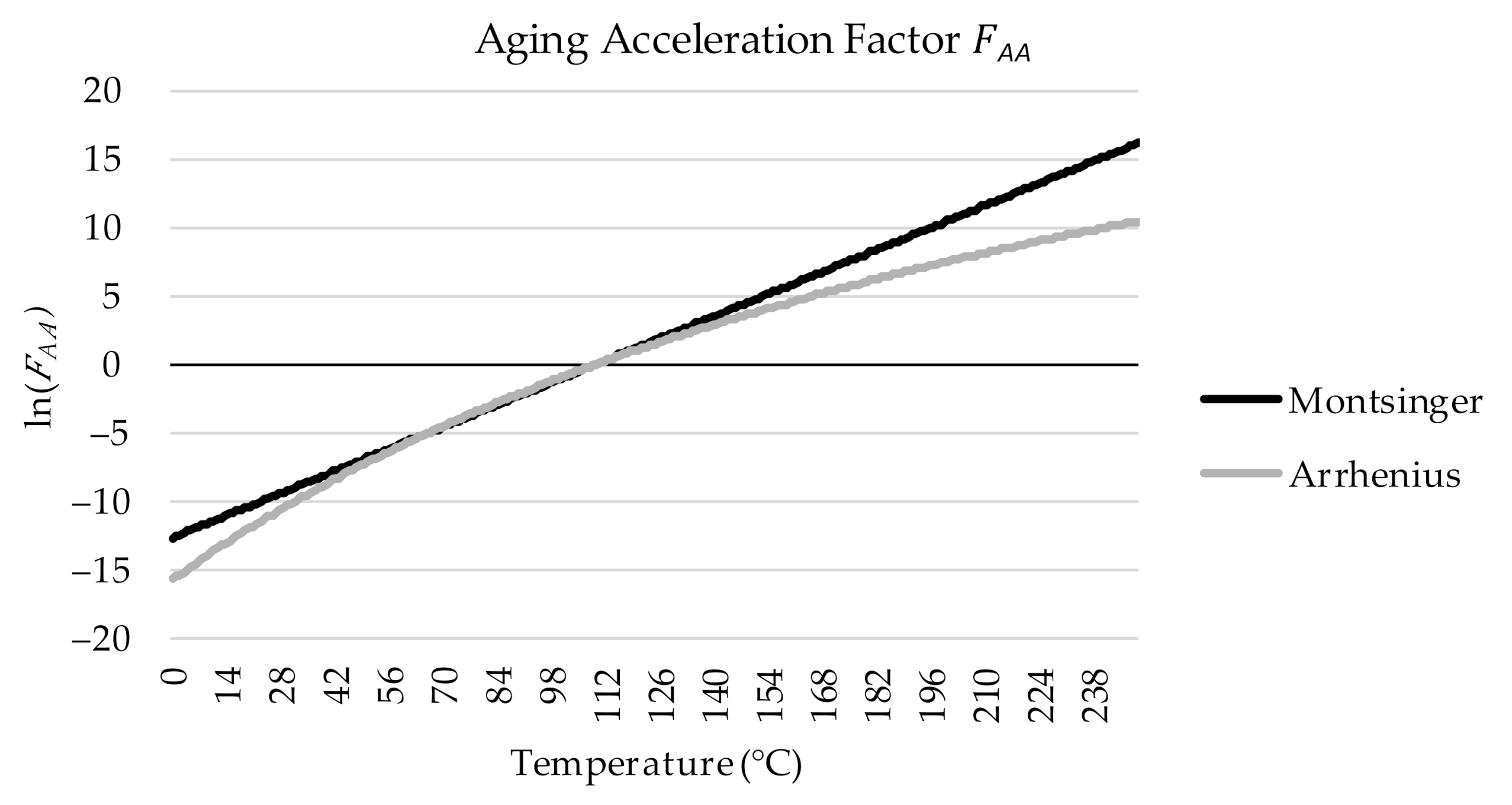
3. Lifetime Assessment of PILC Cables with Regard to Thermal Aging—Methodology

For paper insulated cables, typical age for replacement is about 50 years but varies between 15 and 80 years amongst different DSO. The replacement is mostly based on a technical, economical or strategic criteria (cf. [32,33,34] regarding different maintenance strategies). The often quoted generally accepted lifetime of cables of 40 years is derived from present experience of operated cables. Power cable manufacturers do not specify any expected period of cable lifetime [3].

Aging can be described as a gradual deterioration of the physical and electrical strength of the equipment until failure occurs and the component loses functionality, which marks the end of the equipment’s life [35]. This represents the last part of the so-called bathtub phenomenon. The bathtub curve reflects the development of failure rates with few failures at the beginning of the life cycle, often due to manufacturing defects or bad assembly, followed by a long period during which failures are rare and an increasing number of failures at the end of the lifetime [3].

For cables, a large proportion of defaults are attributable to cable joints. Relating to statistical data of a large DSO in The Netherlands, 45% of failures observed for MV cable systems can be traced back to them [36]. Failures in this regard are not investigated here.

As described in Section 2, thermal degradation is the main aging mechanism for PILC cables. Further degradation, e.g., due to electrical aging, can be determined by multi-stress models (cf. [37,38,39,40]). However, this is not examined further at this point. Instead, a methodology for a lifetime assessment is described exclusively with regard to thermal aging. When determining cable temperatures for thermal aging also increased dielectric losses due to thermal degradation of the insulation (cf. [36,38,41]) are neglected.

The correlation between lifetime and temperature of the considered medium is described by the thermal aging reaction rate $k$, given by the Arrhenius law [42]:

$$\begin{gathered} k=A·e^{\left(\frac{B}{T}\right)} \\ \mathrm{with}: \\ B=\frac{-E_a}{R} \end{gathered}$$

(17)

where $R$ is the universal gas constant and $T$ is the absolute temperature. $A$ and $B$ are component specific constants that are particularly derived from empirical studies [43]. Experimental evidence indicates for transformers with cellulose insulation that $A=9.8\times {10}^{-18}$ and $B=15,000$. With Arrhenius reaction rate theory, per unit life and percentage loss of life can be calculated as follows [44]:

$$\begin{gathered} \mathrm{Per} \mathrm{Unit} \mathrm{Life}=A·e^{\left(\frac{B}{T}\right)}=L\left(T\right) \\ \mathrm{Percentage} \mathrm{Loss} \mathrm{of} \mathrm{Life}=D_t\left(T\right)=\frac{F_{EAA}·\Delta t·100}{L\left(T_{ref}\right)}=\frac{\Delta t·100}{L\left(T\right)} \\ \mathrm{with}: \\ L\left(T\right)=\frac{L\left(T_{ref}\right)}{F_{EAA}} \\ {F}_{EAA}=\frac{{{\displaystyle \sum }}_{n=1}^m{F}_{AA,n}·\Delta t_n}{{{\displaystyle \sum }}_{n=1}^m\Delta t_n} \\ {F}_{AA}=\frac{L\left(T_{ref}\right)}{L\left(T\right)}=e^{\left[\frac{B}{T_{ref}} - \frac{B}{T}\right]} \end{gathered}$$

(18)

where $L\left(T\right)$ is the lifetime at the occurred absolute temperature $T$ and $D_t\left(T_{ref}\right)$ is the percentage loss of life or degradation rate throughout the total time period $\Delta t$ with regard to the reference lifetime $L\left(T_{ref}\right)$ at the reference absolute temperature $T_{ref}$. $F_{AA}$ is the aging acceleration factor—the rate at which insulation aging is accelerated compared with the aging rate at reference temperature. $F_{EAA}$ is the equivalent aging factor for the total number of time intervals $m$ and $F_{AA,n}$ is the aging acceleration factor for the temperatures that exists during the time interval $\Delta t_n$.

The aforementioned formulas according to the Arrhenius law are also applicable for the aging behavior of power cables. The constants $A$ and $B$ could be estimated from historic load data, but these data are usually not available [43]. A novel way to determine these Arrhenius parameters is presented in [19,43], using a simulation of historic cable utilization. The study is carried out for cables with a reference temperature of 90 °C and a corresponding lifetime of 40 years and is therefore not suitable for PILC cables.

The Montsinger rule as an adaption of the Arrhenius law for transformers can also be applied for PILC cables to determine the aging behavior [38,45,46,47]:

$$\begin{gathered} F_{AA}=\frac{D_y\left({\vartheta }_c\right)}{D_y\left({\vartheta }_{ref}\right)}=2^{\left(\frac{{\vartheta }_c-{\vartheta }_{ref}}{{\vartheta }_d}\right)} \\ {D}_y\left({\vartheta }_c\right)=D_y\left({\vartheta }_{ref}\right)·2^{\left(\frac{{\vartheta }_c-{\vartheta }_{ref}}{{\vartheta }_d}\right)} \\ {D}_t\left({\vartheta }_{c,n}\right)=\frac{\frac{{{\displaystyle \sum }}_n^m{2}^{\left(\frac{{\vartheta }_{c,n}-{\vartheta }_{ref}}{{\vartheta }_d}\right)}}{x_n}·t·100}{L\left({\vartheta }_{ref}\right)} \end{gathered}$$

(19)

where $x_n$ is the number of time steps, $D_y\left({\vartheta }_c\right)$ is the yearly degradation rate at conductor temperature ${\vartheta }_c$, $D_y\left({\vartheta }_{ref}\right)$ is the yearly degradation rate at reference temperature and ${\vartheta }_d$ is the temperature increase that doubles the degradation rate. Montsinger has demonstrated a correlation for the aging of paper-oil insulation systems. “He noted that the rate of deterioration of mechanical properties doubled for each 5–10 °C increase in temperature. The doubling factor was not a constant, being about 6 °C in the temperature range from 100–110 °C and 8 °C for temperatures above 120 °C. However, people tend to remember the doubling factor as a constant and the present IEC Loading Guide uses 6 °C” [44].

A comparison between Montsinger rule and Arrhenius law reveals a significant difference, shown in Figure 3. There is only agreement for a small temperature range. Otherwise, the Montsinger rule always yields higher aging in the given case (cf. [46]).

For the calculation of the degeneration rate with regard to thermal aging, the load-dependent conductor temperature ${\vartheta }_{c,n}$ is required analogous to the hottest point temperatures for transformers. The corresponding values are determined with Formula (14), which reflect the conductor temperature under consideration of the thermal time constant at the end of a time step, which is assumed to comprise 300 s (5 min). The resolution of 5 min was chosen to ensure high accuracy for dynamic temperature calculation. These time steps differ from the generation fluctuations considered for DER, for which hourly variations are assumed.

For the lifetime assessment, there is a need for reference data for the service life of the cable at a given temperature. Together with the Arrhenius parameters or Montsinger rule, these variables provide the necessary database for thermal aging. Currently, there is little or no data on this. Further research is needed in this respect, especially since the reference values have a major influence on the final outcome (see Figure 4). At this point, the Montsinger rule and related reference data from the literature are compared with the Arrhenius law and related estimated reference data. For the latter, a service life of 15 years at maximum load is assumed, based on the minimum lifetime for PILC cables under replacement [36]. A continuous load of 100% as well as 70% is regarded as maximum load. In addition, for the Arrhenius parameter $B$ the value according to the transformer insulation from [44] is used. Based on these assumptions, the following calculation for the degeneration according to the Arrhenius Law results:

$$D_t\left({\vartheta }_{c,n}\right)=\frac{\frac{{{\displaystyle \sum }}_n^m{e}^{\left[\frac{B}{{\vartheta }_{ref}+273}-\frac{B}{{\vartheta }_{c,n}+273}\right]}}{x_n}·\Delta t·100}{L\left({\vartheta }_{ref}\right)}=\frac{\frac{{{\displaystyle \sum }}_n^m{e}^{\left[\frac{15,000}{{\vartheta }_{ref}+273}-\frac{15,000}{{\vartheta }_{c,n}+273}\right]}}{x_n}·\Delta t·100}{15 a}$$

(20)

In [45] reference data for the Montsinger rule is given. A yearly degradation rate of 0.5% for PILC cables at a reference temperature of 15 °C and ${\vartheta }_d=6.5 °\mathrm{C}$ is assumed. This corresponds to an expected lifetime at this temperature of 200 years:

$$L\left(T\right)=\frac{F_{EAA}·\Delta t·100}{D_y\left(T_{ref}\right)}=\frac{1·1a·100}{0.5}$$

(21)

A conductor temperature of approx. 15 °C is reached if the surrounding temperature is 10 °C and a load of 30% is present. In relation to the typical age for replacement of PILC cables of 50 years and average utilization rates in the medium-voltage grids of 20 to 35%, a reference lifetime of 200 years (cf. [45]) seems very high. At 15 °C, however, almost no thermal aging takes place. Instead, other aging mechanisms dominate the service life. This explains the high lifetime values when only thermal aging is considered at such low temperatures.

Figure 4 shows the lifetime curves related to the different aging models with the reference data and assumptions presented above.

The curves according to Arrhenius law reflect a cable service life of 15 years with an assumed constant load of 70% (37 °C conductor temperature) on the one hand and of 100% (65 °C conductor temperature) on the other hand as a reference point. Arrhenius constant B has a considerable influence on the slope of the lifetime curve. For comparison, in Figure 4 also a curve with B = 7500 instead of B = 15,000 is included. The reference data for the Arrhenius model are based only on simplified assumptions at this point. For this reason, the Montsinger rule and the reference data given in [45] are used for the lifetime assessment of PILC cables presented in this paper. Lifetime assessment for transformers is also typically performed according to this model. According to the explanations in this chapter, the selected database probably provides extreme values for the thermal aging of PILC cables.

The large deviation of the curves illustrates the significance of the reference data. There is a need for further research on this topic. As more accurate reference data become available, this should be used to review the results of the lifetime assessment in Section 6.

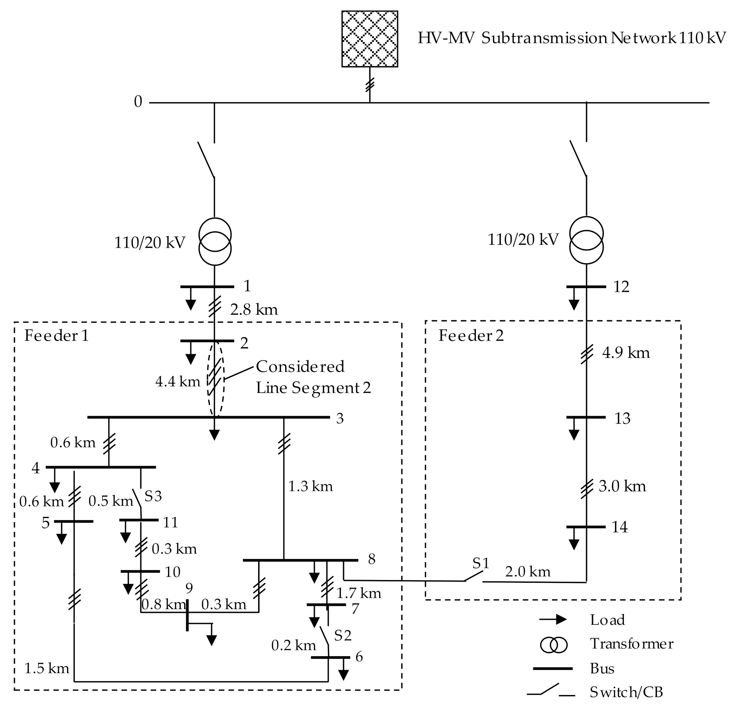
4. MV Distribution Network Benchmark

The CIGRE Task Force C6.04.02 has developed benchmark systems to facilitate the analysis and validation of methods and techniques that enable the economic, robust, and environmentally responsible integration of DER. In [48] network benchmarks for different voltage levels and versions for North American style with 60 Hz and European style with 50 Hz as a common basis for testing are presented. Out of this, the medium voltage (MV) distribution network benchmark with 50 Hz is used to evaluate the aging of PILC cables in case of different load scenarios, shown in Figure 5.

The selected network benchmark represents a typical European medium-voltage grid that is derived from a physical network in southern Germany, which supplies a small town and the surrounding rural area. Depending on the switch position, the network can be operated radially or meshed. At this point the radially version with open switches is considered. The MV distribution network has a nominal voltage of 20 kV and is fed from the 110 kV subtransmission network via separate transformers. XLPE cables (type NA2XS2A) in the area of feeder 1 and aluminum overhead lines in the area of feeder 2 are used as conductors. As an investigation of PILC cables is carried out here, the cable type originally used in the network benchmark is adapted. PILC cables (type NEKEBA 3 × 120 mm² 12/20 kV) with the parameters from

Table 4. PILC cable tested for thermal aging.

Type	${\mathit{R}}_{\mathit{D}\mathit{C}}$ at 20 °C (Ohm/km)	X (Ohm/km)	C (nF/km)	Un (kV)	R0/R1 (p.u.)	X0/X1 (p.u.)	C0 (nF/km)
NEKEBA 3 × 120 mm2	0.157	0.123	338.0	20.0	9.48	3.29	338.0

are chosen for all line segments.

In the MV distribution network benchmark different residential and commercial/industrial loads are included.

Table 5. Load parameters of European MV distribution network benchmark [48].

Node	Apparent Power, S (kVA)		Power Factor
	Residential	Commercial/Industrial	Residential	Commercial/Industrial
1	15,300	5100	0.98	0.95
2	---	---	---	---
3	285	265	0.97	0.85
4	445	---	0.97	---
5	750	---	0.97	---
6	565	---	0.97	---
7	---	90	---	0.85
8	605	---	0.97	---
9	---	675	---	0.85
10	490	80	0.97	0.85
11	340	---	0.97	---
12	15,300	5280	0.98	0.95
13	---	40	---	0.85
14	215	390	0.97	0.85

gives the values of the coincident peak loads for each node of the network. Load values given for nodes 1 and 12 are much higher than those for the other ones, because these loads represent additional feeders that are not modeled in detail. The loads are assumed to be symmetric [48]. Line segments and their corresponding lengths that connect the different network nodes are shown in

Table 6. Connections and line lengths of MV distribution network benchmark [48].

Line Segment	Node from	Node to	Length (km)
1	1	2	2.82
2	2	3	4.42
3	3	4	0.61
4	4	5	0.56
5	5	6	1.54
6	6	7	0.24
7	7	8	1.67
8	8	9	0.32
9	9	10	0.77
10	10	11	0.33
11	11	4	0.49
12	3	8	1.3
13	12	13	4.89
14	13	14	2.99
15	14	8	2

.

In order to limit the scope of the investigations, only a line segment with high utilization is analyzed according to the load scenarios from Section 5. Line segment 2 is selected for the lifetime assessment, which is marked in Figure 5.

Several DER are additionally integrated into the network benchmark. According to the wind power-dominated and photovoltaic dominated scenario, explained in Section 5, the total installed apparent power of all wind power and photovoltaic (PV) plants is chosen. Other DER are neglected because of their limited influence. Single power plants are distributed randomly to nodes of feeder 1 (including node 1) as shown in

Table 7. Distribution of wind power and photovoltaic plants in the MV distribution network.

Node	Name/Type	Installed Apparent Power, S (kVA)
		Wind Power-Dominated	PV-Dominated
Node 1	PV1	2.11	2.83
Node 11	PV11	2.11	2.83
Node 4	PV4	2.11	2.83
Node 5	PV5	2.11	2.83
Node 10	PV10	2.11	2.83
Node 9	PV9	2.11	2.83
Node 8	PV8	2.11	2.83
Node 5	W5	6.5	2.115
Node 3	W3	6.5	2.115
Node 8	W8	6.5	2.115
Node 10	W10	1.5	2.115
Total	Wind power plants (W)	21.0	8.5
	Photovoltaic plants (PV)	14.8	19.8

. In the wind power-dominated scenario, it is necessary to reinforce line segments 1 and 2 to avoid high grid bottlenecks. For this purpose, a parallel PILC cable with an identical configuration according to Table 4 is set up. It is assumed that all plants are connected to the medium-voltage grid. For power generators in this voltage level, a reactive power control according to VDE 4110 is necessary. A voltage-dependent control is selected as shown in Figure 6.

5. Representative Load Scenarios

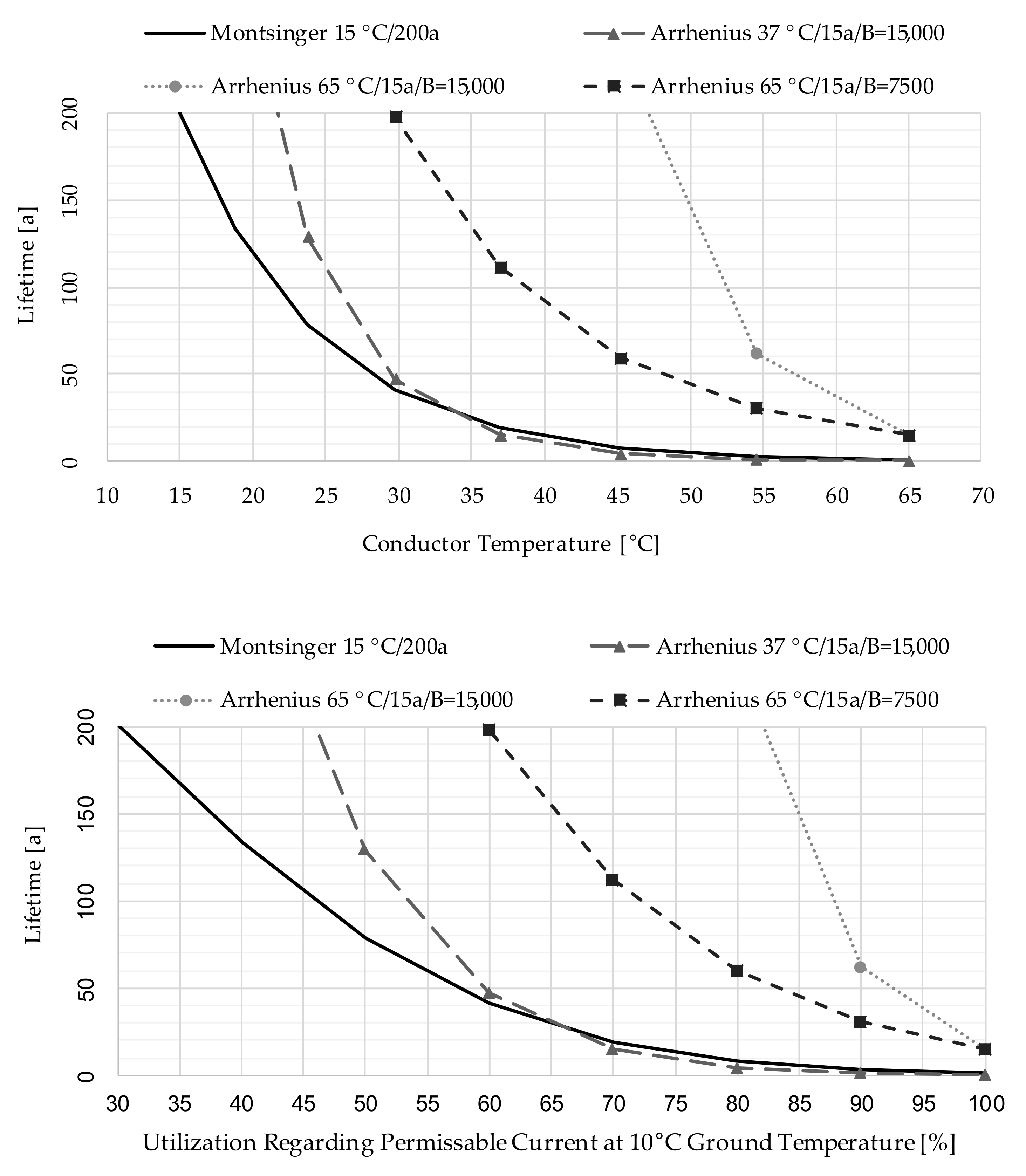
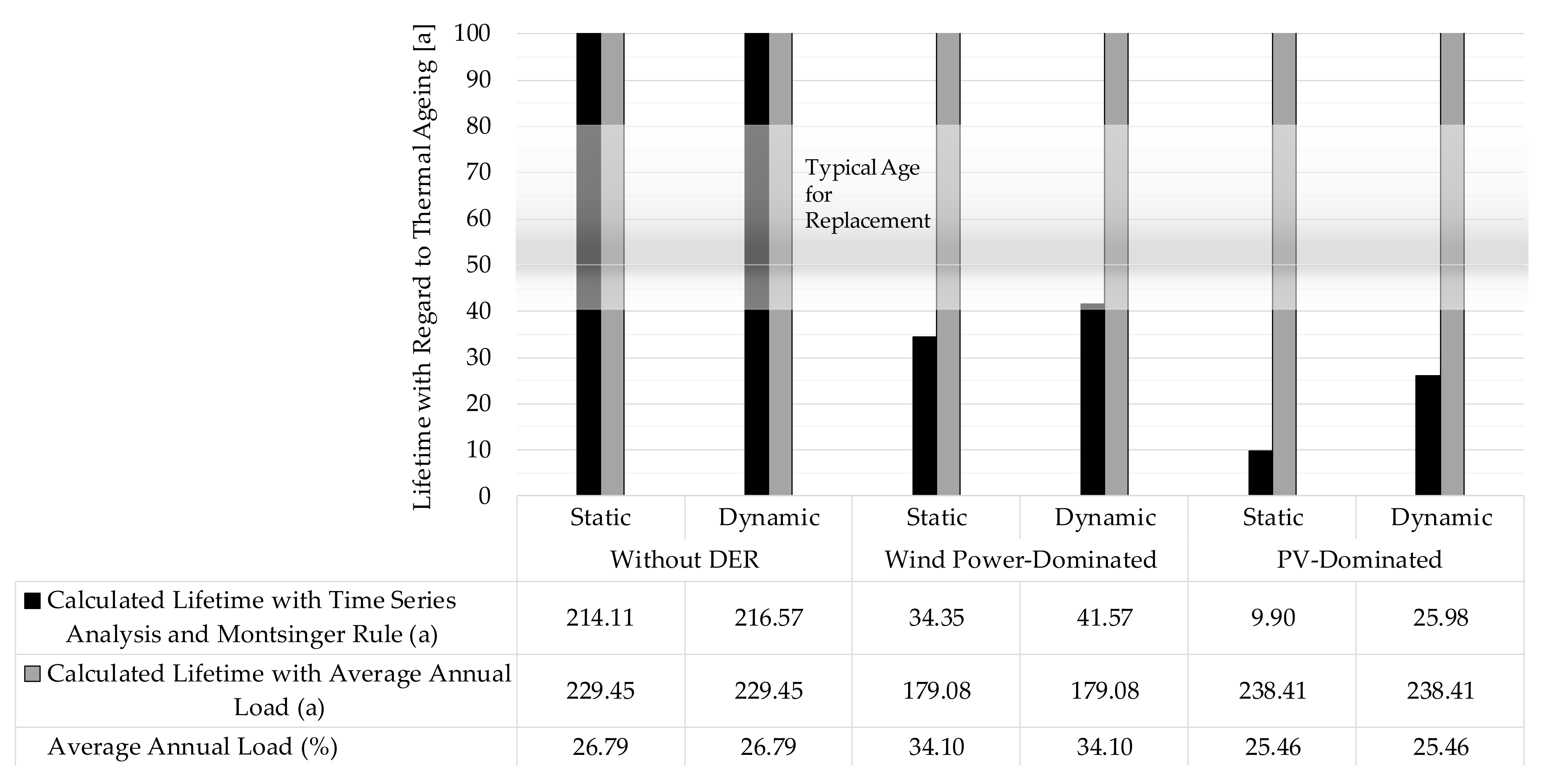
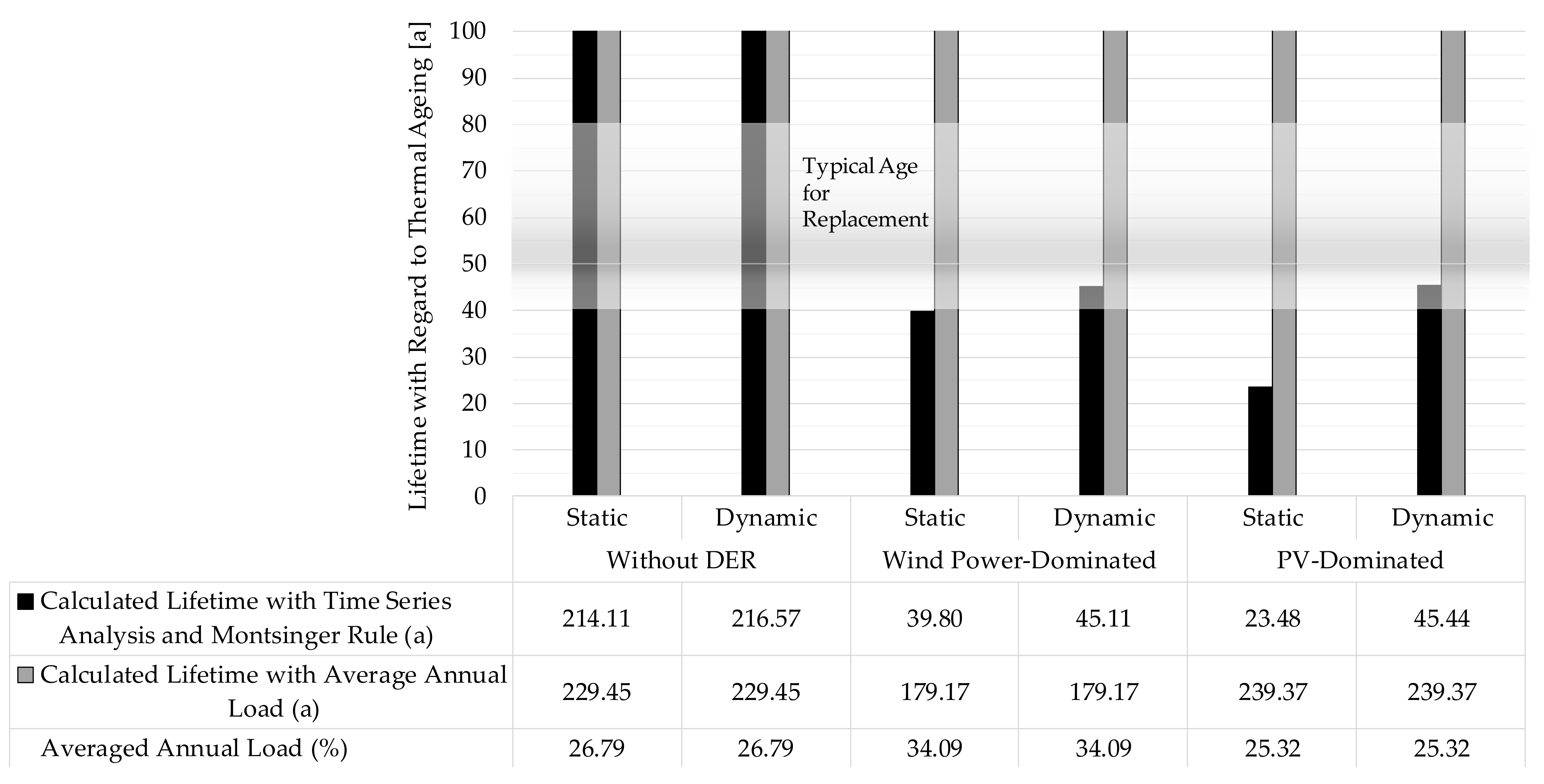
For the lifetime assessment of line segment 2 from the network benchmark different load scenarios are investigated. On the one hand, a scenario is examined without DER, i.e., with a load only by the connected power consumers. On the other hand, the influence of DER is considered by a future prognosis about their penetration.

In [49] three scenarios of the future expansion of DER in Germany until 2032 are presented. These scenarios differ in the total installed capacity and the local distribution of the plants. The scenario “EEG 2014”, for example, is taken into account as a minimal scenario with 128 GW of DER in 2032 (60 GW wind power plants, 59 GW PV plants, 9 GW others). This scenario is used for the lifetime assessment of line segment 2, as the required data is the only publicly available. More recent political objectives in Germany are forcing a comparatively higher level of expansion.

To distribute the total installed apparent power to federal states, grid areas and voltage levels, in [49], an analysis of existing networks and previously installed power plants in Germany is used. Based on this, the expansion of DER is assigned to representative medium-voltage (MV) and low-voltage (LV) model network classes (“Modellnetzklassen”) using stochastic methods. Each of these classes (10 LV and 8 MV classes) represent distribution grids with a similar typical distribution of loads and feed-ins. The ratio of the average installed DER capacity to the annual maximum load for each withdrawal point in the network is used as an adequate indicator of how strongly the load flow in a distribution grid is influenced by DER. For example, this ratio is above 2 in MV model network classes 7 and 8 (see

Table 8. Grid area classes [50].

Grid Area Classes	Characteristics	Model Network Classes from [49]
Wind power-dominated	High feed-ins by photovoltaic and wind power plants; Low load per withdrawal point; Typical for Schleswig-Holstein	4 (LV) + 6 (MV)
Weak Load	Moderate feed-ins by photovoltaic systems and high feed-ins by wind power plants; Low load per withdrawal point; Typical for Eastern Germany (Mecklenburg-Vorpommern and Brandenburg)	3 (LV) + 6 (MV)
PV-dominated	High feed-ins by photovoltaic systems and low feed-ins by wind energy plants; High load per withdrawal point; Typical for Southern Germany (Baden-Württemberg and Bavaria)	Bavaria: 7 (LV) + 8 (MV) Baden-Württemberg: 10 (LV) + 7 (MV)

) related to the installed capacity of photovoltaic plants [49]. The higher the ratio, the greater the need for grid expansion or the number of grid bottlenecks [50]. In [50], grid area classes (“Netzgebietsklassen”) are formed that represent combinations of different model network classes from [49]. Three classes with a strong generation-related need for future grid expansion are detected, listed in Table 8.

With reference to the aforementioned studies, the following scenarios are used for the lifetime assessment presented in Section 6:

• ▪ PV-dominated in Bavaria (MV model network class 8 from [49]),
• ▪ Wind power-dominated in Schleswig-Holstein (MV model network class 6 from [49]).

In [49] the network structure parameters of the MV model network classes are assumed to be 8 branches with 15 withdrawal points each, i.e., a total of 120 withdrawal points. Multiplied with the average installed DER capacity per withdrawal point, the total capacity of wind power and PV plants for the corresponding scenarios or grid area classes emerge, shown in

Table 9. Expected value of installed capacity of DER in in particularly affected MV distribution networks in 2032.

Scenarios/Grid Area Classes	Average Installed DER Capacity per Withdrawal Point According to the Scenario “EEG 2014” from [49]		Total DER Capacity
	Photovoltaic (kW)	Wind Power (kW)	Photovoltaic (MW)	Wind Power (MW)
Wind power-dominated	123.2	178.9	Approx. 15	Approx. 21
PV-dominated	165	70.5	Approx. 20	Approx. 8

. These scenarios reflect the expected expansion of DER for the year 2032 in particularly affected MV network areas in Germany.

In order to create a profile that provides a holistic and realistic view of the loads on a cable, a load flow analysis (Newton–Raphson method) is carried out over one year. Load profiles are required for this purpose. For consumers, the standard load profiles H0 for households and G0 for commercial/industry are selected from [51,52]. The profile H0 is adjusted over the year according to the dynamization function in [51]. The corresponding per unit load curves during the period from Friday to Sunday related to the second week of 2012 are shown in Figure 7 and Figure 8, as well as the annual load curves 2012.

Since the values in Table 5 reflect coincident peak loads, the maximum values of the individual loads are converted with a coincidence factor of 0.85. Using the two standard load profiles H0 and G0, this results in the corresponding simultaneous peak values.

For DER, the generic feed-in profiles for 2030 from [53] are used. This is a federal state specific standard data set for wind power and PV plants for different years of consideration (2020–2050), which was created on the basis of a consistent and transparent modeling. These feed-in profiles reflect hourly fluctuations in power generation of wind power and PV plants. The selected feed-in profiles for Bavaria and Schleswig-Holstein are shown as annual load duration curves in Figure 9.

6. Results

For an exemplary PILC cable (see Table 1 and Table 4) of line segment 2 from the MV distribution network benchmark (see Figure 5 in Section 4), a lifetime assessment with regard to thermal aging is performed. The results are presented in the following. The basis for determining the thermal aging of cables is the conductor or insulation temperature (see Section 2) that results from their utilization.

High utilization or overloads in radially operated distribution networks occur especially in substations and the adjacent line segments, such as line segment 2 in the network benchmark. The utilization of this line segment is determined by means of a load flow analysis for three different load scenarios, namely without DER, wind power- and PV-dominated (see Section 5). The corresponding annual load duration curves of line segment 2 in relation to the permissible current (see Formula (2): $I_p=302 \mathrm{A}·0.88$) are shown in Figure 10. The load limits of the transformer of feeder 1 are not violated, and the maximum utilization is approx. 100%. In the scenarios with DER the highest voltage deviations of approx. −3% and +2% relate to the nominal voltage level occurred at node 11 of the network benchmark. Also at this node, the maximum voltage deviation in the scenario without DER is about −4%.

Without DER the annual load duration curve is relatively flat, with a maximum utilization of approx. 50%. In contrast, the corresponding curves of the scenarios with DER show significant peak values, especially the PV dominated scenario. Peak Loads occur temporarily due to the type of power generation and reach up to 120% of the maximum permissible current in the PV-dominated scenario. Such short-term peaks are taken into account at this point for the lifetime assessment to illustrate the corresponding effect on service life, as some DSO also allow such overloads in practice (see Section 2.2). Alternatively, however, the service life is also evaluated here if the feed-ins are reduced by the DSO so that line segment 2 is utilized to a maximum of 100%.

Figure 11 shows the correlation of the utilization of line segment 2 with the network load of feeder 1 (see Figure 5) for the scenarios wind power-dominated and without DER. Alternatively, the correlation with the network load of the entire MV distribution network benchmark is shown in Figure 12. The network load $P_N$ is calculated as follows:

$$P_N=max\left(\sum P_L,\sum P_F\right)$$

(22)

where $\sum P_L$ is the sum of all withdrawals from loads and network losses and $\sum P_F$ is the sum of all feed-ins in a network area, e.g., feeder 1. The illustrations indicate that without decentralized feed-ins, the network load of an entire distribution network correlates well with the load of a selected individual line. With the penetration of DER, this is usually no longer the case, especially if there are different degrees of expansion of decentralized power plants in subnetwork areas. In the selected example, DER are installed exclusively in feeder 1 to represent an extreme scenario. If DER are in place, the correlation between the network load and the utilization of single line segments exists only if the network load is formed for interconnected network areas (INA, cf. [54]). However, this does not necessarily apply to all line segments of an INA. In areas with few or no feed-ins within an INA, there can be no correlation. This is the case, for example, for line segment 5 and the network load of feeder 1, as shown in Figure 13. For line segment 5, which has a very low utilization rate, the line load correlates with the sum of all withdrawals from loads and network losses $\sum P_L$ (see Formula (22)) from Feeder 1. The correlations presented here can be useful for congestion management in order to assess in which network situations bottlenecks occur.

To determine the conductor temperature of the selected PILC cable type according to the load of line segment 2, the methodology presented in Section 3 is used. Within this approach all heat sources are considered as Joule losses or losses converted therein. This allows a simplified modelling with one heat source. As a further simplification, the drying-out of the soil is ignored. However, in Section 2, formulas are shown to account for this effect. In addition, a constant ground temperature of 10 °C is assumed. This corresponds roughly to the annual mean value in Germany at a depth of 2 m, which has risen from approx. 10 to 12 °C between 1900 and 2020 [55]. A more precise temperature determination could be made by varying the ground temperature during the year, e.g., using Formula (16).

The calculation of the conductor temperature was carried out using both a dynamic and a static calculation method. The dynamic calculation is made according to Formula (14). Thereby a thermal time constant of 2 h (cf. [27]) is taken into account. If lower thermal time constants would apply, e.g., 30 min, only a small deviation from a static analysis would occur (approx. 86% steady-state temperature after $\Delta t=2·\tau$), when hourly load fluctuations are considered. For comparison with the dynamic computation, a static calculation is also performed according to Formula (13). The conductor temperatures resulting from both calculation methods with an exemplary course of the cable load is shown in Figure 14. The figure illustrates the significant effect when thermal time constants are respected.

Based on the conductor temperature, the service life of the PILC cable is determined using the Montsinger rule according to Formula (19) and the reference data from [45]. As described in Section 3, there is an urgent need for solid reference data for aging models of PILC cables.

Figure 15 presents the different resulting lifetimes for the three analyzed load scenarios if a maximum utilization of 120% is allowed, whereby a distinction is made between static and dynamic temperature calculation. In addition, the service life calculated with the average annual load instead of time series values is included in the figure. Currently, this approach is commonly used by DSO to estimate the degeneration of cables. As Figure 15 shows, this methodology leads to approximately identical lifetimes compared to a time series analysis for a load scenario without DER. Also, in this scenario only slight differences result to the lifetimes with static compared to dynamic temperature calculation. The small differences can be explained essentially by the relatively flat annual load duration curve.

In principle, however, the thermal aging in the scenario without DER is negligible so that no relevant reduction in service life due to the load is to be expected. Other aging mechanisms determine the lifetime of the cable in this case. If only thermal aging is examined, like it is done at this point, very high lifetimes result. Typically, PILC cables are replaced after 50 years and after 80 years at the latest [3].

For load scenarios with DER, the service life of the PILC cable differs tremendously between an assessment according to the average annual load and time series analysis. The annual average utilization even decreases due to the integration of DER in the PV dominated scenario. In contrast, the peak load increases clearly. The lifetime values in Figure 15 indicates that the high peak loads accelerate the degeneration of PILC cables significantly, even if these are only temporarily occurring. This is due to the fact that the thermal aging increases exponentially with load. The service life is particularly low in the PV-dominated scenario. Here, peak loads occur more frequently than in the wind power-dominated scenario. Furthermore, substantial discrepancies between the static and dynamic temperature calculation method can be seen. The results show that thermal time constants urgently need to be taken into account in the lifetime assessment of cables with regard to thermal aging. Otherwise the service life would be assessed to low.

When evaluating the results presented in this section, it should be noted that the lifetime data represent extreme values. The load on the line segment under consideration represents an extremum. DSO could reduce the feed-ins during operation to avoid peak loads. This is often permissible to the extent that only a certain proportion of the energy volume generated annually by decentralized generation plants is allowed to be reduced, e.g., 3%. In this context, an additional lifetime assessment was performed under the condition that a DSO allows a maximum utilization of 100% of the cable under consideration. In order to ensure this, less than 3% of the annual amount of energy generated by DER must be reduced. The results are shown in Figure 16. They indicate that the service life of the cable can be significantly increased by avoiding overloads. The service life is approx. 45 years in both DER scenarios, covering nearly the typical service life of PILC cables currently in use with the previous load without DER.

If overloading is prevented, the maximum temperature of the conductor is always below 65 °C. If an overload of 20% is allowed, the maximum temperature is approx. 78 °C in the wind power-dominated and approx. 85 °C in the PV-dominated scenario. The temperatures are additionally about 7 °C higher, if a static calculation without thermal time constants is performed.

For all results of the lifetime assessment it has to be considered that an additional consideration of the fluctuating soil temperatures during the course of the year and the drying-out of the soil could lead to higher peak conductor or insulation temperatures and thus to a higher degradation. Furthermore, the results of the lifetime estimation presented in this section should only be considered as an approximation if the selected reference data from [45] for the aging model are actually applicable.

7. Discussion and Outlook

In this paper, the thermal aging of PILC cables under the influence of DER is considered for extreme scenarios. In networks with DER short-term peak loads on electrical equipment can occur, even if the average load does not necessarily rise. For PILC cables this could lead to significantly increased thermal aging. This is due to the fact that thermal aging increases exponentially with utilization of PILC cables. Excessive aging of PILC cables due to the influence of DER could already be reduced by preventing overloads in a few hours of a year by means of generation or load management. In order to achieve this in a cost-optimized way, a compromise between the aging costs and the costs of the energy management should be considered. The maximum permissible load on the electrical equipment should be limited so that the costs of the corresponding accelerated aging do not exceed the benefit of the higher transmission capacity. The results of the lifetime estimation presented in this paper should only be considered as an approximation if the selected reference data from the literature for the aging model are actually applicable.

Usually, lifetime assessment of PILC cables is performed based on the average annual load. It is shown in this paper that this approach is only suitable for load situations without DER, and that a time series analysis can overcome the shortcomings in situation with decentralized and fluctuating feed-ins from wind power or PV plants. The determination of thermal aging is based on the calculation of the conductor or insulation temperature. The consideration of thermal time constants has a significant influence on the determination of the temperature and the corresponding thermal aging. If the thermal dynamics are not taken into account, the estimated service life turns out to be considerably too low.

Beyond the methodology used in this paper, the accuracy of the lifetime assessment can be further improved by taking into account the fluctuating soil temperatures over the course of the year and the drying-out of the soil. An approach to how this can be achieved by using correction factors is also shown in this paper. If these influences are taken into account, this could lead to higher resulting peak temperatures and greater degeneration than without them. A possible approach to dealing with varying soil temperatures throughout the year could be to allow different maximum cable loads depending on the season.

In addition to the influence of DER, the methodology described in this paper could also be used to determine the influence of consumers with high power requirements, e.g., electric vehicle charging stations, on the thermal aging or service life of PILC cables.

References

1. Chmura, L.A. Life-Cycle Assessment of High-Voltage Assets Using Statistical Tools. Ph.D. Thesis, Delft University of Technology, Delft, The Netherlands, 2014. [Google Scholar]
2. FGH. Forschungsgemeinschaft für Elektrische Anlagen und Stromwirtschaft e.V. Zustandsdiagnose von Papiermasse-Kabelanlagen im Verteilungsnetzen. In Technischer Bericht 300; FGH: Mannheim, Germany, 2006. [Google Scholar]
3. Conseil International des Grands Réseaux Électriques. Remaining Life Management of existing AC Underground Lines. Technical Brochures; CIGRÉ: Paris, Franch, 2008. [Google Scholar]
4. Künstl, B. Stromtragfähigkeitsgrenzen von Elektrischen Leitungssystemen. Diplomarbeit; Technische Universität Graz; Institut für Hochspannungstechnik und Systemmanagement: Graz, Austria, 2011. [Google Scholar]
5. Adam, R.; Großmann, S.; Haller, R. Beitrag zur Thermischen Dimensionierung von Niederspannungs-Schaltgerätekombinationen. Ph.D. Thesis, Technische Universität Dresden, Dresden, Germany, 2019. [Google Scholar]
6. Oeding, D.; Oswald, B.R. Elektrische Kraftwerke und Netze, 8. Auflage; Springer Vieweg: Berlin, Germany, 2016; ISBN 9783662527030. [Google Scholar]
7. Brüggmann, J. Wechselspannungstechnologiebasierte Bipolare Mehrphasensysteme. Ph.D. Thesis, Universität Duisburg-Essen, Essen, Germany, 2012. [Google Scholar]
8. Linenbrink, T.L. The history and mystery of the Neher-McGrath formula. Consult.-Specif. Eng. 2014, 51, 46–52. [Google Scholar]
9. Schermeyer, H. Netzengpassmanagement in Regenerativ Geprägten Energiesystemen. Untersuchungen zur Abregelung Erneuerbarer Energien und zur Sektorenkopplung in Einem Deutschen Verteilnetz. Ph.D. Thesis, Karlsruher Instituts für Technologie (KIT), Karlsruhe, Germany, 2018. [Google Scholar]
10. Schäfer, K.F. Netzberechnung: Verfahren zur Berechnung elektrischer Energieversorgungsnetze, 1st ed.; Springer Vieweg: Wiesbaden, Germany, 2020; ISBN 365826733X. [Google Scholar]
11. Sillaber, A. Leitfaden zur Verteilnetzplanung und Systemgestaltung. Entwicklung dezentraler Elektrizitätssysteme; Springer Vieweg: Wiesbaden, Germany, 2016; ISBN 9783658147136. [Google Scholar]
12. Woschitz, R.; Schichler, U.; Pirker, A.; Komar, G. FEM-Simulation des Thermischen Langzeitverhaltens von Hochspannungs-Kabelanlagen bei Laständerungen; Symposium Energieinnovation: Graz, Austria, 2016. [Google Scholar]
13. Czaap, S. Effect of soil moisture on current-carrying capacity of low-voltage power cables. Prz. Elektrotech. 2019, 1, 156–161. [Google Scholar] [CrossRef]
14. Lindström, L. Evaluating Impact on Ampacity According to IEC-60287 Regarding Thermally Unfavourable Placement of Power Cables; KTH Electrical Engineering: Stockholm, Sweden, 2011. [Google Scholar]
15. Cichowski, R.R.; Kliesch, M. Kabelhandbuch; EW Medien und Kongresse: Frankfurt, Germany, 2012; ISBN 9783802210563. [Google Scholar]
16. Schlabbach, J. Elektroenergieversorgung. Betriebsmittel, Netze, Kennzahlen und Auswirkungen der Elektrischen Energieversorgung, 3rd ed.; VDE-Verl.: Berlin, Germany, 2009; ISBN 9783800731084. [Google Scholar]
17. Scheffler, J. Verteilnetze auf dem Weg zum Flächenkraftwerk. Rechtlicher Rahmen, Erzeuger, Netze; Springer: Berlin/Heidelberg, Germany, 2016; ISBN 9783642552960. [Google Scholar]
18. Heinhold, L. Kabel und Leitungen für Starkstrom, 4th ed.; Siemens AG: Berlin, Germany, 1989; ISBN 3800915243. [Google Scholar]
19. Buhari, M. Reliability Assessment of Ageing Distribution Cable for Replacement in Smart Distribution Systems; University of Manchester: Manchester, UK, 2016. [Google Scholar]
20. Tang, W.H.; Wu, Q.H. Condition Monitoring and Assessment of Power Transformers Using Computational Intelligence; Springer: London, UK, 2011; ISBN 9780857290519. [Google Scholar]
21. Heizmann, T. Berechnungsmethoden für Auslegung, Betrieb und Sicherheit von Elektrischen Energieversorgungssystemen. Thermische Berechnung von Kabelanlagen; FKH-/VSE—Fachtagung: Zürich, Switzerland, 2011. [Google Scholar]
22. Hruška, M.; Clauser, C.; De Doncker, R.W. The Effect of Drying around Power Cables on the Vadose Zone Temperature. Vad. Zone J. 2018, 17, 180105. [Google Scholar] [CrossRef] [Green Version]
23. Rerak, M.; Ocłoń, P.; Taler, J.; Węglowski, B.; Sobota, T. The effect of soil and cable backfill thermal conductivity on the temperature distribution in underground cable system. E3S Web Conf. 2017, 13, 2004. [Google Scholar] [CrossRef] [Green Version]
24. Rummich, E. Energiespeicher: Grundlagen, Komponenten, Systeme und Anwendungen, 2nd ed.; Expert Verlag: Renningen, Germany, 2015; ISBN 9783816932970. [Google Scholar]
25. Schröder, D. Elektrische Antriebe—Grundlagen, 6th ed.; Springer Viewg: Berlin, Germany, 2017; ISBN 9783662554487. [Google Scholar]
26. Specovius, J. Grundkurs Leistungselektronik. Bauelemente, Schaltungen und Systeme, 8, Erweiterte und Aktualisierte Auflage; Springer Vieweg: Wiesbaden, Germany, 2017; ISBN 9783658169114. [Google Scholar]
27. Wieben, E. Multivariates Zeitreihenmodell des Aggregierten Elektrischen Leistungsbedarfes von Standardverbrauchern für die Probabilistische Lastflussberechnung. Ph.D. Thesis, Technische Universität Clausthal, Clausthal-Zellerfeld, Germany, 2008. [Google Scholar]
28. Sami, T.; Gholami, A.; Shahrtash, S.M. Effect of electro-thermal, load cycling and thermal transients stresses on high voltage XLPE and EPR power cable life. In Proceedings of the 8th International Conference on Advances in Power System Control, Operation and Management (APSCOM 2009), Hong Kong, China, 8–11 November 2009; pp. 1–6. [Google Scholar] [CrossRef]
29. Ma, K.; He, N.; Liserre, M.; Blaabjerg, F. Frequency-Domain Thermal Modeling and Characterization of Power Semiconductor Devices. IEEE Trans. Power Electron. 2016, 31, 7183–7193. [Google Scholar] [CrossRef]
30. Kerber, G. Aufnahmefähigkeit von Niederspannungsverteilnetzen für die Einspeisung aus Photovoltaikkleinanlagen. Ph.D. Thesis, Technische Universität München, München, Germany, 2011. [Google Scholar]
31. Recknagel, H.; Schramek, E.-R. Taschenbuch für Heizung und Klimatechnik. Einschließlich Warmwasser- und Kältetechnik, 73rd ed.; Oldenbourg: München, Germany, 2007; ISBN 9783835631045. [Google Scholar]
32. Müller, A.-C.; Weindl, C.; Linossier, J.P.; Schramm, J.; Benkert, L. Requirements of a system for the artificial ageing of paper insulated lead covered medium voltage cables. In Proceedings of the 2018 International Conference on Diagnostics in Electrical Engineering (Diagnostika), Pilsen, Czech Republic, 4–7 September 2018; pp. 1–4, ISBN 978-1-5386-4423-2. [Google Scholar]
33. Stötzel, M. Strategische Ressourcendimensionierung von Netzleitstellen in Verteilungsnetzen, 1st ed.; Gerettete Schriften-Verl. epubli GmbH: Wuppertal, Germany, 2014; ISBN 9783844278262. [Google Scholar]
34. Balzer, G.; Schorn, C. Asset Management für Infrastrukturanlagen—Energie und Wasser, 3rd ed.; Springer: Berlin, Germany, 2020; ISBN 9783662615263. [Google Scholar]
35. Willis, H.L.; Welch, G.V.; Schrieber, R.R. Aging Power Delivery Infrastructures; CRC Press: New York, NY, USA, 2001; ISBN 0824705394. [Google Scholar]
36. Chmura, L.; Morshuis, P.H.F.; Mehairjan, R.P.Y.; Smit, J.J. Review of the residual life assessment of high-voltage cables by means of bottom-up and top-down analysis—Dutch experience. Gaodianya Jishu 2015, 41, 1114–1124. [Google Scholar]
37. Feilat, E.A. Lifetime Assessment of Electrical Insulation. In Electric Field; Kandelousi, M.S., Ed.; IntechOpen: London, UK, 2018; ISBN 978-1-78923-186-1. [Google Scholar]
38. Chmura, L.; Jin, H.; Cichecki, P.; Smit, J.; Gulski, E.; Vries, F. Use of dissipation factor for life consumption assessment and future life modeling of oil-filled high-voltage power cables. IEEE Electr. Insul. Mag. 2012, 28, 27–37. [Google Scholar] [CrossRef]
39. Mazzanti, G. The combination of electro-thermal stress, load cycling and thermal transients and its effects on the life of high voltage ac cables. IEEE Trans. Dielect. Electr. Insul. 2009, 16, 1168–1179. [Google Scholar] [CrossRef]
40. Mazzanti, G. Analysis of the Combined Effects of Load Cycling, Thermal Transients, and Electrothermal Stress on Life Expectancy of High-Voltage AC Cables. IEEE Trans. Power Deliv. 2007, 22, 2000–2009. [Google Scholar] [CrossRef]
41. Houtepen, R.; Chmura, L.; Smit, J.J.; Quak, B.; Seitz, P.P.; Gulski, E. Estimation of dielectric loss using damped AC voltages. IEEE Electr. Insul. Mag. 2011, 27, 20–25. [Google Scholar] [CrossRef]
42. Densley, J. Ageing mechanisms and diagnostics for power cables—An overview. IEEE Electr. Insul. Mag. 2001, 17, 14–22. [Google Scholar] [CrossRef]
43. Buhari, M.; Levi, V.; Awadallah, S.K.E. Modelling of Ageing Distribution Cable for Replacement Planning. IEEE Trans. Power Syst. 2016, 31, 3996–4004. [Google Scholar] [CrossRef]
44. Institute of Electrical and Electronics Engineers. IEEE Guide for Loading Mineral.-Oil-Immersed Transformers and Step-Voltage Regulators; C57.91-2011 (Revision of IEEE Std C57.91-1995); IEEE: New York, NY, USA, 2012; ISBN 78-0-7381-7195-1. [Google Scholar]
45. Huifei, J. Application of Dielectric Loss Measurements for Life Consumption and Future Life Estimation Modeling of Oil-Impregnated Paper Insulation in HV Power Cables. Master’s Thesis, Delft University of Technology, Delft, The Netherlands, 2010. [Google Scholar]
46. Hayder, T.; Radakovic, Z.; Schiel, L.; Feser, K. Einfluss der Kurzschlussdauer auf die Alterung eines Transformators; Elektrie: Berlin, Germany, 2003; Volume 57. [Google Scholar]
47. Weindl, C. Verfahren zur Bestimmung des Alterungsverhaltens und zur Diagnose von Betriebsmitteln der Elektrischen Energieversorgung. Habilitation; Friedrich-Alexander Universität: Erlangen-Nürnberg, Germany, 2012. [Google Scholar]
48. Conseil international des grands réseaux électriques. Benchmark Systems for Network Integration of Renewable and Distributed Energy Resources; CIGRÉ: Paris, Franch, 2014; ISBN 2858732701. [Google Scholar]
49. Büchner, J.; Katzfey, J.; Flörcken, O.; Moser, A.; Schuster, H.; Dierkes, S.; van Leeuwen, T.; Verheggen, L.; Uslar, M.; van Amelsvoort, M. Moderne Verteilernetze für Deutschland (Verteilernetzstudie): Abschlussbericht. Available online: https://www.bmwi.de/Redaktion/DE/Publikationen/Studien/verteilernetzstudie.pdf?__blob=publicationFile&v=5 (accessed on 23 October 2019).
50. Ecofys; Fraunhofer IWES. Smart-Market-Design in Deutschen Verteilnetzen: Entwicklung und Bewertung von Smart Markets und Ableitung einer Regulatory Roadmap. Available online: https://www.agora-energiewende.de/fileadmin2/Projekte/2016/Smart_Markets/Agora_Smart-Market-Design_WEB.pdf (accessed on 23 October 2019).
51. BDEW. Bundesverband der Energie- und Wasserwirtschaft e.V. Repräsentative VDEW-Lastprofile: VDEW-Materialie M-32/99. Available online: https://www.bdew.de/media/documents/1999_Repraesentative-VDEW-Lastprofile.pdf (accessed on 10 February 2020).
52. BDEW. Bundesverband der Energie- und Wasserwirtschaft e.V. Anwendung der Repräsentativen VDEW-Lastprofile Step by step: VDEW-Materialie M-05/2000. Available online: https://www.bdew.de/media/documents/2000131_Anwendung-repraesentativen_Lastprofile-Step-by-step.pdf (accessed on 10 February 2020).
53. Koch, M.; Tambke, J. Erstellung Generischer EE-Strom-Einspeisezeitreihen mit Unterschiedlichem Grad an Fluktuierendem Stromangebot. Available online: https://www.oeko.de/aktuelles/2016/daten-zur-einspeisung-erneuerbarer-energien (accessed on 21 September 2020).
54. Zapf, M.; Weindl, C.; Pengg, H.; German, R. Specific Grid Charges for Controllable Loads in Smart Grids: A Proposal for a Reform of the Grid Charges in Germany. In Proceedings of the NEIS 2018 Conference on Sustainable Energy Supply and Energy Storage Systems, Hamburg, Germany, 20–21 September 2018; pp. 237–242, ISBN 978-3-8007-4822-8. [Google Scholar]
55. Potsdam Institute for Climate Impact Research (PIK) e. V. Bodentemperatur: Jahresmittelwerte. Available online: https://www.pik-potsdam.de/de/produkte/klima-wetter-potsdam/klimazeitreihen/bodentemperatur (accessed on 16 September 2020).
Figure 1. Temperature curve during heating (left) and cooling (right).
Energies 14 00494 g001
Figure 2. Thermal network models, following [26].
Energies 14 00494 g002
Figure 3. Aging acceleration factor according to Arrhenius reaction rate theory (B = 15,000) and Montsinger rule ( T d = 6   ° C ) at a reference hottest point temperature of 110 °C.
Energies 14 00494 g003
Figure 4. Lifetime regarding different reference data and aging models.
Energies 14 00494 g004
Figure 5. Topology of European MV distribution network benchmark, following [48].
Energies 14 00494 g005
Figure 6. Voltage-dependent reactive power control for power generators in the medium-voltage grid.
Energies 14 00494 g006
Figure 7. Load profile H0 for households, following [51].
Energies 14 00494 g007
Figure 8. Load profile G0 for commercial/industry, following [51].
Energies 14 00494 g008
Figure 9. Annual load duration curve of feed-in profiles from [53] for wind power and PV plants.
Energies 14 00494 g009
Figure 10. Annual load duration curves of line segment 2 for different load scenarios.
Energies 14 00494 g010
Figure 11. Correlation of the load of line segment 2 with the network load of feeder 1 for the scenarios wind power-dominated (left) and without DER (right).
Energies 14 00494 g011
Figure 12. Correlation of the load of line segment 2 with the network load of the entire MV distribution network benchmark for the scenarios wind power-dominated (left) and without DER (right).
Energies 14 00494 g012
Figure 13. Correlation of the load of line segment 5 with the network load (left) and the sum of all withdrawals from loads and network losses (right) from Feeder 1.
Energies 14 00494 g013
Figure 14. Comparison of the static and dynamic conductor temperature calculation method.
Energies 14 00494 g014
Figure 15. Calculated lifetime for the exemplary PILC cable of line segment 2 regarding different reference data and aging models if a maximum utilization of 120% is allowed (typical age for replacement from [3]).
Energies 14 00494 g015
Figure 16. Calculated Lifetime for the exemplary PILC cable of line segment 2 regarding different reference data and aging models if a maximum utilization of 100% is allowed (typical age for replacement from [3]).
Energies 14 00494 g016