Modeling and Dynamic Simulation of a Hybrid Liquid Desiccant System with Non-Adiabatic Falling-Film Air-Solution Contactors for Air Conditioning Applications in Buildings

Abstract

This paper presents an experimentally validated, dynamic model of a hybrid liquid desiccant system. For this purpose, we developed new components for the air-solution contactors, which are of the non-adiabatic falling-film type with horizontal tubes (made of improved polypropylene) and the solution tanks. We also provide new experimental correlations for both the tube-solution heat transfer coefficient and the mass transfer coefficient on the airside as a function of the air velocity. To validate the model, the results obtained from the dynamic simulations were compared with those obtained by monitoring a demonstration unit installed in a sports center in Taipei (Taiwan). Once validated, the model was used to perform a sensitivity analysis at different operational conditions, such as the inlet water temperatures in the air-solution contactors and the LiCl mass fraction at which the system operates. The results of the sensitivity analysis were used to optimize the seasonal performance in terms of comfort and energy required by the system. Compared with a conventional air-handling unit that controls air temperature and humidity, the annual energy savings of the liquid desiccant systems are 17%.

1. Introduction

Liquid desiccant systems (LDS) are interesting air conditioning systems (HVAC) when dehumidification has an important role in the thermal loads because they can achieve a low level of humidity and be driven by low-grade heat sources [1,2,3,4]. Therefore, LDS are highly recommended for humid climates and/or in buildings where low humidity is required. The main components of an LDS are the absorber and the regenerator, where the moist air is dehumidified, and the liquid desiccant is regenerated, respectively. Both processes take place by direct contact between the humid air and the liquid desiccant material.

The combination of LDS with vapor compression refrigeration systems is called a hybrid liquid desiccant system (HLDS). In these systems, the LDS typically handles the latent load, and the vapor compression systems, the sensible load [5]. The cooling demand required to provide the supply air conditions of temperature and humidity is lower than that for conventional systems, so the evaporator of the vapor compression chiller can operate at higher temperatures (which enhances the coefficient of performance -COP- of the system), and post-heating is not required. Therefore, HLDS handles the temperature and humidity control more efficiently than conventional HVAC systems [6]. For all these reasons, it has been shown that HLDS has enhanced COP by between 23.1% and 73.8% and made energy savings of between 26% and 80% [7].

Air-solution contactors of most commercial LDS systems are usually of the adiabatic packed-bed type [8,9,10]. This is because of their simplicity, high contact surface, and low cost. However, Lowenstein [11] listed the main advantages of non-adiabatic air-solution contactors over adiabatic packed-beds. In summary:

• Lower air-pressure drops.
• Lower liquid desiccant flow rates are needed to achieve the same dehumidification/regeneration because the liquid desiccant temperature is kept almost constant along with the air-solution contactor. This previous advantage leads to higher LDS COP and lowers carryover of liquid desiccant.

For these reasons, non-adiabatic air-solution contactors have been studied in more detail [12,13,14,15,16,17]. However, liquid desiccants are highly corrosive to most metal materials. Consequently, alternative materials, such as plastics, have been investigated [13,17,18,19]. However, plastics have two limitations: low thermal conductivity and poor tube wetting. Recently, our group studied the heat and mass transfer performance of a polypropylene absorber with a plasma surface treatment developed by Guerriero and Fina [20] that improves the wettability of polypropylene when it comes into contact with LiCl/H₂O solution. Air cooling and air dehumidification were found to improve by between 35% and 52% in comparison to standard polypropylene [14].

The absorption of moisture in liquid desiccants is driven by a difference between the surface vapor pressure of the desiccant aqueous solution and the water pressure of the surrounding moist air. When the vapor pressure at the desiccant surface is lower than that of the humid air, the desiccant attracts moisture. Conversely, the liquid desiccant releases moisture when the vapor pressure at its surface is higher than that of the surrounding air. In general, the lower the liquid desiccant temperature and the higher the liquid desiccant mass fraction, the lower the vapor pressure and, therefore, the higher the moisture absorption. For this reason, absorber and regenerator temperatures (that is, liquid desiccant temperatures) are interesting variables to be evaluated when analyzing the performance of LDS.

LDS have typically been analyzed by discrete steady-state simulations [21]. In these simulations, parametric studies can be made of system performance as a function of various key parameters (e.g., ambient conditions or working temperatures) [22,23]. However, dynamic simulation enables the seasonal performance of a system to be determined [24,25,26,27] as well as the best control strategies in terms of energy-saving or comfort level [28,29,30,31,32]. Dynamic simulations are particularly useful for LDS because, most of the time, they operate in transient conditions.

HLDS can easily achieve the independent control of temperature and humidity, according to the review presented by Muhammad et al. [33]. According to their literature review, they concluded that dehumidification is more sensitive to the inlet solution temperature in the absorber. They also concluded that the optimization in the control set-points is one of the main points to be considered to improve the overall performance of LDS under dynamic air processing conditions.

In this paper, we present an experimentally validated dynamic model of an HLDS developed on TRNSYS. To model the air-solution contactors, new correlations for the heat and mass transfer coefficients were experimentally obtained. The dynamic model was validated with real measurement data of a new demonstration unit of an HLDS, which consisted of non-adiabatic air-solution contactors with polypropylene tubes subject to a plasma surface treatment that enhanced the wettability of the tubes. The validated model was used to perform a sensitivity analysis as a function of the HLDS inlet water temperatures and the minimum mass fraction required for the regenerator to operate. Next, the working conditions of the system were chosen by performing a multi-objective optimization to minimize both the energy consumption of the system and the discomfort hours. The seasonal performance of the HLDS with optimized working conditions is also presented. The thermal energy requirements of this system are finally compared with those of a conventional air handling unit.

2. Materials and Methods

2.1. Description of the HLDS

Figure 1 illustrates a simple scheme of the HLDS studied, which was coupled to a heat pump that provided heating to the regenerator and cooling to the absorber. The system was installed in two locker rooms of a sports center in Taipei (Taiwan). The HLDS contained non-adiabatic air-solution contactors of the falling-film type with horizontal tubes made of polypropylene. The main novelty of this system is that the polypropylene tubes were subject to a plasma surface treatment [20] to increase their wettability. Although it is usually difficult to maintain the hydrophilicity of the plasma surface treatment over time, so far, after more than three years of operation, the dehumidification performance of the system has not been reduced. In a previous study [14], we found that this treatment enhances both the heat and mass transfer of the air-solution contactors.

Another innovation in this system is how the HLDS is coupled to the heat pump. The evaporator of the heat pump provides the absorber with cooling, and the condenser provides the regenerator with heating. At the same time, the hydraulic circuit is installed in such a way that it can provide either chilled water from the evaporator or hot water from the condenser of the heat pump to the coil inside the air handling unit in accordance with the supply air temperature requirements.

The liquid desiccant material used is a solution of LiCl/H₂O. In addition, the air handling unit of the variable air volume type controls the supply air temperature with a cooling/heating coil and the airflow rate with air fans. The return air from the locker rooms is used to regenerate the solution through the regenerator. In summary, the HLDS is thought to be fully integrated, providing high flexibility for all the possible requirements and independent control of temperature and humidity. Data about the operation of the system has been collected from the demonstration site in Taipei since November 2015 with time intervals of one minute.

2.2. Modeling of the HLDS

Figure 2 illustrates a simplified scheme of the HLDS modeled in this study. The heat pump model was not considered since temperatures and flow rates of the hydraulic circuit were taken from measurements and, therefore, can be used directly for the validation of the rest of the system.

On the other hand, the conditioned zone (see Section 2.2.6) did have to be modeled because the return air was used to regenerate the liquid desiccant material through the regenerator, and the room dry-bulb temperature was used to control the system. Most of the elements of the system are available either in the standard TRNSYS libraries [31] or TESS libraries [32], with the exception of the solution tanks and the air-solution contactors, which have been created for this purpose. These new models are described in the sections below.

2.2.1. Modeling of the Air-Solution Contactors

A new component for the non-adiabatic air-solution contactors was developed in FORTRAN to be used in TRNSYS. The physical processes in the absorber and the regenerator are very similar, but the opposite. For instance, heating is required to regenerate the solution, while cooling is required to dehumidify the air. For this reason, the same equations have been used for both components.

The mathematical model is based on the one described by Hellmann and Grossman [34]. This means that the same equation inputs and outputs were considered. The main reason why this model was used is that it is relatively simple because it can be modeled with algebraic equations. It has also been experimentally validated in [13]. Furthermore, the thermophysical properties of LiCl/H₂O brine (density, enthalpy, specific heat capacity, and viscosity) were adopted from the formulations by Conde [35].

Table 1. Equations used for modeling the air-solution contactors (adapted from [33]).

Water mass balance	${\dot{m}}_{s,out}·\left(1-X_{s,out}\right)-{\dot{m}}_{s,in}·\left(1-X_{s,in}\right)+{\dot{m}}_{a,in}·\left(W_{a,out}-W_{a,in}\right)=0$	(1)
Desiccant material mass balance	${\dot{m}}_{s,out}·X_{s,out}={\dot{m}}_{s,in}·X_{s,out}$	(2)
Energy balance	${\dot{m}}_{w,in}·\left(h_{w,out}-h_{w,in}\right)+{\dot{m}}_{s,out}·h_{s,out}-{\dot{m}}_{s,in}·h_{s,in}+{\dot{m}}_{a,in}·\left(h_{a,out}-h_{a,in}\right)=0$	(3)
Air-solution interface mass balance at the top	${\beta }_{Is}A·\left(X_{s,in}-X_{I,t}\right)-{\sigma }_{a}A·\left(W_{a,out}-W_{I,t}\right)=0$	(4)
Interface mass balance at the bottom	${\beta }_{Is}A·\left(X_{s,out}-X_{I,b}\right)-{\sigma }_{a}A·\left(W_{a,in}-W_{I,b}\right)=0$	(5)
Interface energy balance at the top	$$\begin{gathered} {\alpha }_{a}A·\left(T_{a,out}-T_{I,t}\right)-{\alpha }_{is}A·\left(T_{I,t}-T_{s,in}\right)+{\sigma }_{a}A·\left(W_{a,out}-W_{I,t}\right)·h_{WAi,t} \\ ={\beta }_{is}A·\left(X_{s,in}-X_{I,t}\right)·h_{WSI,t} \end{gathered}$$	(6)
Interface energy balance at the bottom	$$\begin{gathered} {\alpha }_{a}A·\left(T_{a,in}-T_{I,b}\right)-{\alpha }_{Is}A·\left(T_{I,b}-T_{s,out}\right)+{\sigma }_{a}A·\left(W_{a,in}-W_{I,b}\right)·h_{WAI,b} \\ ={\beta }_{Is}A·\left(X_{s,out}-X_{I,b}\right)·h_{WSI,b} \end{gathered}$$	(7)
Water vapor pressure equilibrium at the top	$p_{WS}\left(X_{I,t},T_{I,t}\right)=p_{WA}\left(W_{I,t}\right)$	(8)
Water vapor pressure equilibrium at the bottom	$p_{WS}\left(X_{I,b},T_{I,b}\right)=p_{WA}(W_{I,b})$	(9)
Tube-solution heat transfer equation	$$\begin{gathered} {\dot{m}}_{w,in}·c_{p,w,in}·\left(T_{w,out}-T_{w,in}\right)=UA·{1000}^{-1}·\left(T_{s,in}-T_{w,out}-T_{s,out}+ \\ {T}_{w,in}\right)·(ln{\left(\left(T_{s,in}-T_{w,out}\right)·{\left(T_{s,out}-T_{w,in}\right)}^{-1}\right)}^{-1} \end{gathered}$$	(10)
Air-solution mass transfer equation	$$\begin{gathered} -{\sigma }_a·A·{\dot{m}}_{a,in}^{-1} = ln \left[1 - \left(W_{a,out} - W_{a,in} - W_{I,t} + W_{I,b}\right)·{\left(W_{I,b} - \\ W_{a,in} - \left(W_{I,t} - W_{I,b}\right)·{\dot{m}}_{a,in}·{\left({\sigma }_a·A\right)}^{-1}\right)}^{-1}\right] \end{gathered}$$-	(11)
Air-solution heat transfer equation	$$\begin{gathered} -{\sigma }_a·A·{\dot{m}}_{a,in}^{-1} = ln \left[1 - \left(h_{a,out} - h_{a,in} - h_{I,t} + h_{I,b}\right)·{\left(h_{I,b} - h_{a,in} - \\ \left(h_{I,t} - h_{I,b}\right)·{\dot{m}}_{a,in}·{\left({\sigma }_a·A\right)}^{-1}\right)}^{-1}\right] \end{gathered}$$-	(12)

contains the 12 equations required to obtain the 12 variables calculated: the outlet water temperature ($T_{w,out}$), the outlet moist air humidity ratio ($W_{a,out}$), the outlet moist air temperature ($T_{a,out}$), the outlet solution mass flow rate (${\dot{m}}_{s,out}$), the outlet solution temperature ($T_{s,out}$), the outlet solution mass fraction ($X_{s,out}$), the air-solution interface temperature at the top ($T_{I,t}$), the air-solution interface mass fraction at the top ($X_{I,t}$), the air-solution interface humidity ratio at the top ($W_{I,t}$), the air-solution interface temperature at the bottom ($T_{I,b}$), the air-solution interface mass fraction at the bottom ($X_{I,b}$) and the air-solution interface humidity ratio at the bottom ($W_{I,b}$). The multivariable Newton-Raphson method was used to solve the system of equations.

Moreover, heat and mass transfer coefficients are required. The overall heat transfer coefficient between the water and the film (U) was calculated considering the thermal resistance of water inside the tubes (R_wt), the thermal resistance of the tube wall (R_t), and the thermal resistance of the film outside the tubes (R_ts). The thermal conductivity of the water, λ_w, was obtained using correlations from [36]. Depending on the water flow regime, the Nusselt number was calculated using the empirical correlations for internal forced convection in cylindrical pipes available in Nellis and Klein [37]:

If Re_wt is lower than 2300, then:

$$N{u}_{w-t} = 4.36 + \left(\left(0.1156 + 0.08569·{\left(P{r}_w^{0.4}\right)}^{-1}\right)·G{z}_w\right)·{\left(1 + 0.1158·G{z}_w^{0.6}\right)}^{-1})-$$

(13)

If Re_wt is between 2300 and 10,000, then:

$$N{u}_{w-t} = \epsilon /8·\left(R{e}_w - 1000\right)·P{r}_w·{\left(1+12.7·{\left(\frac{\epsilon }{8}\right)}^{0.5}·\left(P{r}_w^{\frac{2}{3}}-1\right)\right)}^{-1}$$

(14)

If Re_wt is higher than 10,000, then:

$$\mathit{N}{\mathit{u}}_{\mathit{w}\mathbf{-}\mathit{t}} = \mathbf{0.023}\mathbf{·}\mathit{R}{\mathit{e}}_{\mathit{w}}^{\mathbf{0.8}}·\mathit{P}{\mathit{r}}_{\mathit{w}}^{\mathit{n}}-$$

(15)

ε is the pipe friction coefficient which is calculated as:

$$\mathit{\epsilon }={\left(\mathbf{0.79}\mathbf{·}\mathit{l}\mathit{n}\mathit{R}{\mathit{e}}_{\mathit{w}}\mathbf{-}\mathbf{1.64}\right)}^{\mathbf{-}\mathbf{2}}$$

(16)

n is a constant that is equal to 0.4 for heating the water (absorber conditions) and 0.3 for cooling the water (regenerator conditions).

The thermal resistance of the tube wall R_t was calculated with the following expression:

$${\mathit{R}}_{\mathit{t}}=\frac{{\mathit{d}}_{\mathit{o}}}{\mathbf{2}{\mathit{\lambda }}_{\mathit{t}}}\mathbf{·}\mathit{l}\mathit{n}\left(\frac{{\mathit{d}}_{\mathit{o}}}{{\mathit{d}}_{\mathit{i}}}\right)$$

(17)

Since the solution-tube thermal resistance and the mass transfer coefficient in the airside depend on the wetting of the tube surface, correlations for these two coefficients had to be determined for these specific air-solution contactors.

The solution-tube thermal resistance was obtained from the measurements of the air-solution contactors of the HLDS presented in this paper. The data measurement used to obtain the correlations (18) and (19) can be found in [6]. The specifications of both air-solution contactors (absorber and regenerator) are listed in

Table 2. Specifications of the air-solution contactors.

Tube Material	Polypropylene Tubes with Plasma Surface Treatment [14]
Contact surface (m2)	59.29
Tube thermal conductivity (W·(m·°C)−1)	0.21
Tube length (m)	0.68
Bundle width (m)	0.90
Inside tube diameter (mm)	5.10
Outside tube diameter (mm)	6.50

. The correlation obtained for the solution-tube thermal resistance (R_t-s) as a function of the air velocity is expressed as:

$${\mathit{R}}_{\mathit{t}\mathbf{-}\mathit{s}}=\mathbf{165.5}\mathbf{·}{\mathit{v}}_{\mathit{a}}{}^{\mathbf{0.51}}$$

(18)

Similarly, the mass transfer coefficient on the airside was correlated as a function of the air velocity:

$${\mathit{\sigma }}_{\mathit{a}}=\mathbf{2.06}\mathbf{·}{\mathbf{10}}^{\mathbf{-}\mathbf{2}}\mathbf{·}{\mathit{v}}_{\mathit{a}}{}^{\mathbf{1.02}}$$

(19)

The heat transfer coefficient between the air-solution interface and moist air was obtained by using the Chilton-Colburn analogy, in which convective heat transfer and mass transfer coefficients are related by the Lewis number according to the following expression:

$${\mathit{\alpha }}_{\mathit{a}}={\mathit{c}}_{\mathit{p}\mathbf{,}\mathit{a}}\mathbf{·}{\mathit{\sigma }}_{\mathit{a}}\mathbf{·}\mathit{L}{\mathit{e}}_{\mathit{a}}^{\mathbf{2}\mathbf{/}\mathbf{3}}$$

(20)

Because the Lewis number is much higher in the solution film than in the air, the thermal resistance between the interface and the solution can be neglected. Therefore, as Hellman and Grossman suggested in [34], the heat transfer coefficient between the LiCl/H₂O solution and the air-solution interface was set 500 times higher than the heat transfer coefficient between the air-solution interface and moist air. They also showed that the mass transfer coefficient between the air-solution interface and the solution could be assumed to be three times lower than the mass transfer coefficient of the solution.

The left-hand graph in Figure 3 shows a comparison between the dehumidification achieved by the absorber at steady-state conditions and the dehumidification calculated by using the mathematical model and equations given above. According to this graph, the deviations between measured and calculated dehumidification were, in most cases, lower than 5%. Similarly, the right-hand graph in Figure 3 shows a comparison between the heat duty achieved by the absorber at steady-state conditions and the heat duty calculated using the same model. In this case, deviations between measured and calculated heat were always lower than 2.5%. As in the absorber, deviations of the water regenerated, and the heating required between measurements at steady-state conditions and calculated by the model were lower than 5% in almost all the cases. These deviations were in the range of the measurement uncertainties.

2.2.2. Modeling of the Liquid Desiccant Tanks

The energy storage capacity of the solution tanks is related not only to the temperature of the liquid desiccant but also to the liquid desiccant mass fraction. As a consequence, the model of the liquid desiccant tanks must consider that both the mass inside them and the liquid desiccant mass fraction are changeable. The solution tanks have two inlet streams and one outlet stream.

The solution tanks model was based on energy and LiCl and total mass balance equations. Moreover, complete mixing was assumed. The calculation of the water mass considered the amount of water content in the previous time step (−1) and the mass balance of water in the tank at that time. Therefore, the mass balance was calculated at every time step as:

$$\begin{gathered} M_w=M_{w,-1}+{\displaystyle \int }[{\dot{m}}_{in,1}·\left(1-X_{in,1}\right)+{\dot{m}}_{in,2}·\left(1-X_{in,2}\right)-{\dot{m}}_{out} \\ ·\left(1-X_{tank,-1}\right)]·dt \end{gathered}$$

(21)

$$X_{tank}=\frac{M_{LiCl}}{M_{tank}}$$

(22)

To calculate the tank temperature at every time step, the energy balance in the tank was formulated considering the temperature of the tank at the previous time step. This means:

$$\begin{gathered} T_{tank}=T_{tank,-1}+{\displaystyle \int }\left[\frac{{\dot{m}}_{in,1}·T_{in,1}}{M_{tank}}+\frac{{\dot{m}}_{in,2}·T_{in,2}}{M_{tank}}-\frac{{\dot{m}}_{out}·T_{out}}{M_{tank}} \\ -\frac{U{A}_{tank}·\left(T_{tank,-1}-T_{amb}\right)}{M_{tank,-1}·c_{p,s}}\right]·dt \end{gathered}$$

(23)

To achieve convergence along with the simulation and to ensure the accuracy of the results, we set a simulation time step (6 s).

Table 3. Specifications of the liquid desiccant tanks.

Parameter	Value
Initial mass (kg)	200
Initial LiCl mass fraction (%)	35%
Initial temperature (°C)	25
Specific heat of the solution (kJ·(kg·°C)−1) [35]	2.71
Overall heat transfer coefficient (kW·°C−1)	0.021

contains the parameters of the liquid desiccant tanks for the simulations. The initial mass value of the solution tank was the amount of liquid desiccant added to the system during its operation in the demo site in Taipei. The overall heat transfer coefficient of the solution tanks was adjusted by evaluating the evolution of the liquid desiccant temperature measured inside the solution and the ambient temperature.

2.2.3. Modeling of Other Components

As well as the air-solution contactors and the solution tanks, other components were included in the system model. All the components described in this section were taken from standard TRNSYS libraries or TESS libraries.

The solution heat exchanger and the air-air heat exchanger were modeled with the standard component Type91. The cooling/heating coil was modeled with the standard component Type5d.

Table 4. Specifications of the heat exchangers.

Parameter	Solution Heat Exchanger	Air–Air Heat Exchanger	Cooling/Heating Coil
Cold side specific heat (kJ·(kg·°C)−1)	2.72	1.02	4.19
Hot side specific heat (kJ·(kg·°C)−1)	2.66	1.02	1.02
Effectiveness (-)	0.83	0.67	-
Overall heat transfer coefficient (kW·°C−1)	-	-	1.00

contains the specifications of the heat exchangers.

The hydraulic components of the LDS are the two pumps that take the liquid desiccant from the solution tanks and two diverting valves that distribute the liquid desiccant flow through the different branches of the circuit. The pumps were modeled with Type3b, which is a constant flow rate pump. The liquid desiccant flow rate was set at 2.5 kg/s, which agrees with the measured values of the system. The diverting valves were modeled with Type647 from the TESS libraries. The split ratio, which is the recirculated solution flow divided by the total solution flow, was set at 0.93 for the two diverting valves of the circuit.

2.2.4. Modeling of the Control Strategy

One of the main advantages of dynamic simulations is that they can include the control strategy in the model. Two different standard components were used to implement the control:

• Type2d, which is a generic differential on/off controller. This component was used to start/stop the regeneration process as a function of the LiCl mass fraction at the inlet of the absorber with a dead hysteresis band of 2.5%.
• Type2b, which is a temperature differential on/off controller. This component was used to set the operational mode of the system—that is, heating or cooling—as a function of the room temperature with a dead hysteresis band of 2 °C.

In addition, a PID component (Type23 of standard libraries) was included in the model for three different controls:

• To set the airflow rate as a function of the room set-point temperature (25 °C).
• To set the water flow rate at the inlet of the absorber as a function of the room set-point humidity ratio (0.010 kg_w/kg_da).
• To set the water flow rate at the inlet of the cooling/heating coil as a function of the supply air set-point temperature (19 °C in summer conditions and 31 °C in winter conditions).

Gain, derivative, and integral constants of the proportional-integral-derivative (PID) controllers were separately tuned to improve their actuation. Moreover, the maximum and minimum values for the water and airflow rates in the PID controllers are in agreement with the fans and pumps specifications of the experimental installation.

2.2.5. Modeling of the Ambient Conditions

The dry bulb temperature and relative humidity were measured every minute for a whole year. These measured data were used for dynamic simulations. As a summary of the weather conditions, Figure 4 shows the monthly mean ambient temperature and humidity ratio collected by the sensors. As can be observed, both the ambient temperature and the humidity ratio were very high for six months (from May to October), with mean ambient temperatures higher than 30 °C and mean humidity ratios of about 0.020 kg_w/kg_da during these months. The other months were cooler and drier, with mean ambient temperatures and humidity ratios around 20 °C and 0.012 kg_w/kg_da, respectively.

2.2.6. Modeling of the Internal Loads

To model the internal loads of the locker rooms, Type759 from the TESS libraries was used. This component calculates the room air temperature and humidity levels using two differential equations to solve the heat and mass balances. The user must provide internal loads and ventilation conditions. In this case, the internal loads and the ventilation conditions were calculated from real data taken during the system operation time. The internal loads were calculated from the measured supply and return air conditions (airflow, air temperature, and humidity ratio) obtained from monitoring the demonstration unit for a whole year with a measurement time step of 1 min.

Figure 5 shows the monthly internal loads (sensible cooling, sensible heating, and latent cooling) of the room. It is essential to mention that this room was closed in February for one week, for two weeks in August, and three weeks in December. As can be seen from this Figure, latent loads were always present and represented a significant amount of the total loads. However, sensible heating was more important from January to March and sensible cooling, from April to November.

3. Results

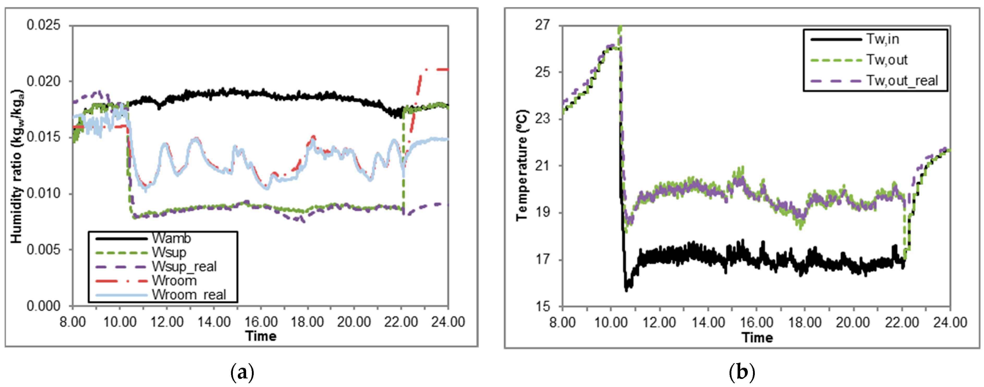
3.1. Validation of the Model

To validate the model, outputs calculated from simulations were compared with real measurements of the system during operation. The left-hand graph in Figure 6 shows the comparison between the air humidity ratios (supply and room values) calculated from the dynamic simulation and the measurements of the real system for a typical day. Similarly, the right-hand graph in Figure 6 shows the comparison between the absorber water temperature calculated from the dynamic simulation and the measured values for the same day of operation. According to the results, discrepancies between the calculated and measured humidity ratios and absorber water temperatures were very small. The differences found between W_sup and W_room after 22:00 are because the system was shut down at this time.

Table 5. Statistical comparison between measured and simulated data of some parameters of the system.

Statistical Parameter	Wsup (kgw·kgda−1)	Wroom (kgw·kgda−1)	Tsup (°C)	Troom (°C)	Tw,out,abs (°C)	Tw,out,reg (°C)
Standard deviation	0.0004	0.0003	0.3	0.3	0.2	0.1
Average calculated	0.0088	0.0129	20.6	25.6	19.7	49.3
Average measured	0.0086	0.0127	21.2	25.9	19.7	49.5

also shows a statistical comparison between the results obtained by the simulated model and the measured data during operation. In the same way, as in the figures above, the compared variables are a good approximation of the modeled HLDS.

We also made a monthly and an annual comparison between the energy transferred within the main components of the system (that is, the absorber, the regenerator, and the heating/cooling coil). As an example, Figure 7 shows this comparison for three different months: February, which is the coolest and driest month; April, which is an intermediate month; and June, the warmest and most humid month. As can be seen in this Figure, for these three months, the discrepancies between the measured and the calculated results were small. In the same way, the measured and the estimated annual results showed small differences between them, as can be observed in Figure 7. Comparison between calculated and measured monthly energy transferred in the main components of the system during February (a), April (b), and June (c).

Table 6. Annual difference between the measured and calculated energy transferred.

	Absorber	Regenerator	Cooling Coil	Heating Coil
Energy transferred difference (%)	4.9	9.9	11.1	5.2

, which contains the yearly difference between the energy transfer measured and calculated as a percentage.

These results show that the system can be regarded as validated. Therefore, in the sections below, the model is used to make a sensitivity analysis of the system in different working conditions.

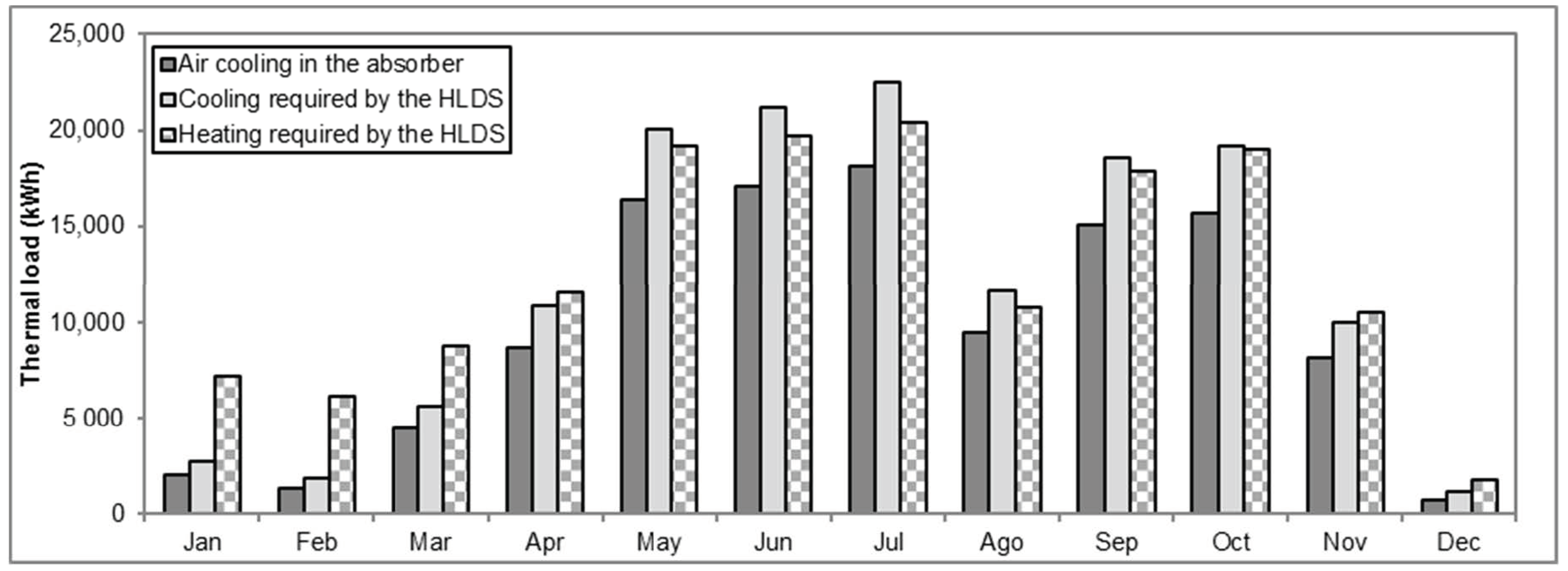
3.2. Sensitivity Analysis

We used the model to perform a sensitivity analysis of three operational variables of the system: the minimum LiCl mass fraction at the entrance to the absorber (a variable that is used to activate the regeneration process), the inlet water temperature in the absorber, and the cooling coil and the inlet water temperature in the regenerator and the heating coil. In this regard, the system was simulated at 45 operational conditions. The inlet water temperature in the absorber ranged from 12 °C to 16 °C, and inlet water temperature in the regenerator ranged from 51 °C to 55 °C. These temperature values are in agreement with the working temperatures that the heat pump can provide. The minimum LiCl mass fraction ranged from 25% to 35%. The maximum LiCl mass fraction at the entrance to the absorber (a variable that stops the regeneration process) was set 2.5% higher than the minimum LiCl mass fraction.

The following annual variables of the system were analyzed:

• The heating required by the HLDS, which is the annual heating needed in the regenerator and the heating coil.
• The cooling required by the HLDS is the annual cooling needed in the absorber and the cooling coil.
• The air cooling (sensible + latent) in the absorber.
• The number of hours in discomfort conditions.

Conditions were regarded as being uncomfortable whenever the room temperature was higher than 26 °C or lower than 22 °C or whenever the room humidity ratio was higher than 0.012 kg_w/kg_da. These criteria are in agreement with those suggested by ASHRAE [38].

Illustration (a) in Figure 8 shows the heating required by the HLDS as a function of the three operational parameters evaluated. The minimum LiCl mass fraction at the entrance to the absorber was the parameter with the greatest effect: the higher the minimum LiCl mass fraction, the higher the heating required by the HLDS. This effect is because more energy is required to regenerate more water from the desiccant. Furthermore, the higher the inlet water temperature in the regenerator, the higher the annual heating required in the regenerator. This effect is due to an increase in water regeneration at high water temperatures. Inlet water temperature in the absorber did not show any significant effect on the heating required by the HLDS.

As is shown in illustration (c) of Figure 8, both the inlet water temperature in the regenerator and the LiCl mass fraction at the entrance to the absorber were the variables that most affect air cooling in the absorber. The higher the inlet water temperature in the regenerator, the higher the air cooling in the absorber. This effect is due to the higher air dehumidification achieved in the absorber because of greater water regeneration. On the other hand, the air cooling in the absorber reached a maximum at medium values of the minimum LiCl mass fraction at the entrance to the absorber. This is due to two opposite factors: (1) high LiCl mass fractions decrease the sensible cooling of moist air in dry months, and (2) low LiCl mass fractions decrease the latent cooling of moist air in hot and humid months.

Similarly, graph (b) in Figure 8 illustrates the annual cooling required by the HLDS. In this case, since the cooling required was the cooling added to the absorber and the cooling coil, the lower sensible cooling observed in the absorber for the higher LiCl mass fractions at the entrance of the absorber was compensated by the sensible cooling provided in the cooling coil. This is why the cooling required by the HLDS remained stable when LiCl mass fractions were high. Moreover, the inlet water temperature at the entrance to the absorber also affects the cooling energy required because the cooling provided to the air through the cooling coil was greater at lower temperatures.

Finally, graph (d) in Figure 8 shows the number of hours in discomfort conditions as a function of the three operational variables evaluated. The number of hours in comfort conditions was inversely correlated to the cooling required by the HLDS: the lower the number of hours, the higher the inlet water temperatures in the regenerator, the lower the inlet water temperatures in the absorber, the higher the minimum LiCl mass fractions at the entrance to the absorber.

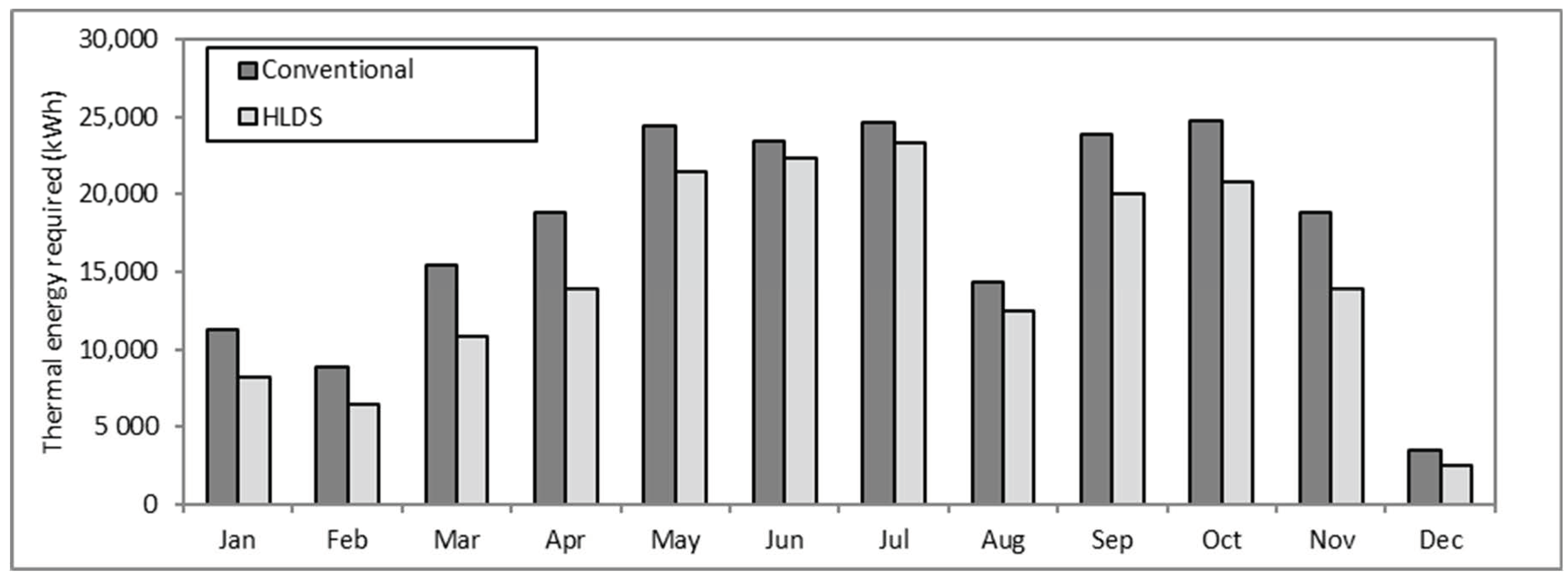
3.3. Optimization and Annual Results

To select the operational conditions that optimize the seasonal performance of the system, the results of the previous sensitivity analysis were used in a multi-objective optimization analysis. The two graphs in Figure 9 illustrate the hours in discomfort conditions as a function of the cooling (left) and the heating (right) required by the HLDS. Since the three variables should be minimized, the Pareto front multi-objective optimization method can be used. The darker points represent the operational conditions that coincide with the Pareto front in both graphs. In this case, the number of hours out of comfort conditions was chosen as lower than 300. With this requirement, the selected point was the value with a better ratio between the required energy and the number of discomfort hours.

The selected point corresponded to an inlet water temperature in the absorber equal to 12 °C, an inlet water temperature in the regenerator equal to 55 °C, and a minimum LiCl mass fraction equal to 30%.

Table 7. Annual results of the HLDS working in the optimized working conditions.

Annual Result	Value
Heating required by the HLDS (kW·h)	152,950
Cooling required by the HLDS (kW·h)	145,462
Total number of hours in discomfort conditions	262.6
Air cooling provided in the absorber (kW·h)	117,370

contains the annual results of the HLDS working in the optimized working conditions.

Figure 10 shows the monthly results of the system at the same working conditions. Since the system does not recirculate any air from the room, the thermal loads were significantly affected by the ambient conditions. During summer, the cooling required by the HLDS was greater than the heating. However, during the winter, the heating required was more than twice the cooling. This difference is due not only to the heating in the coil but also to the heating in the regenerator, which was higher in the winter months than the heat duty in the absorber. This suggests that a control strategy that changes the operational conditions throughout the year could increase the seasonal performance of the system. Finally, most of the total cooling required was provided by the absorber. There are two reasons for this: latent cooling is higher than sensible cooling, and part of the sensible cooling is provided by the absorber.

4. Discussion

When a conventional air handling unit (CS) has to control both the moist air humidity and temperature, it requires two devices: a cooling coil that cools the air below the dew point to dehumidify it to the set-point supply air humidity ratio, and a heating coil to achieve the set-point supply air temperature. A CS is less efficient than an HLDS, which dehumidifies moist air without first having to decrease its temperature (see Figure 11).

To evaluate the energy savings of the HLDS studied, it was compared with a CS in terms of the thermal energy required by the two systems. Since the compared cases require both cooling (to dehumidify the air in the CS and to dehumidify and cool the air in the HLDS) and heating (to heat the air in the CS and to regenerate the liquid desiccant in the HLDS), we assumed that both systems were coupled by a water-to-water heat pump. Therefore, the comparison was made by quantifying the maximum thermal load (heating or cooling) for each time step, assuming that the minimum thermal load was provided by the waste heat of the same heat pump. Once the maximum demand was obtained for each time step, they were integrated for every month and the whole year to calculate the energy savings.

For the comparison between the two systems to be fair, the supply air conditions of both systems were required to handle the internal loads (sensible and latent loads). The assumptions in the energy consumption calculation in the CS are summarized in

Table 8. Assumptions made for the conventional air handling unit.

Parameter	Value
Cooling coil bypass factor (-)	0.08
Supply chilled water temperature (°C)	7.0
Return chilled water temperature (°C)	12.0

.

According to the results, the annual thermal energy saving achieved by the HLDS was 36,021 kWh, 16.97% of the CS energy requirements. As can be seen in Figure 12, the highest energy savings were mostly for months with moderate ambient conditions, such as March (29.60%) or November (26.55%). Moreover, the thermal energy required for the HLDS was always lower than for the CS.

The HLDS was also compared with the CS in terms of exergy efficiency. Since the HLDS was working most of the time at transient conditions, the comparison of the exergy efficiency was made at nominal conditions.

Table 9. Nominal conditions for the exergy efficiency calculation.

Parameter	Value
Ambient air temperature (°C)	31.0
Ambient air humidity ratio (kgw/kgda)	0.0190
Air flow rate (kg/s)	0.875
Supply air temperature (°C)	17.73
Supply air humidity ratio (kgw/kgda)	0.0084
Room air temperature (°C)	26.0
Room air humidity ratio (kgw/kgda)	0.0110

shows these conditions. Operational conditions of the HLDS correspond with the selected in Section 3.3 for the HLDS and Table for the CS.

The exergy efficiency for the HLDS was calculated as:

$${\eta }_{Ex,HLDS} = \left(E{x}_{sup} - E{x}_{amb}\right)·{\left(E{x}_{abs,in} + E{x}_{ccoil,in} - E{x}_{abs,out} - E{x}_{ccoil,out}\right)}^{-1}$$

(24)

The exergy efficiency for the CS was calculated as:

$${\eta }_{Ex,CS} = \left(E{x}_{sup}- E{x}_{amb}\right)·{\left(E{x}_{ccoil,in} - E{x}_{ccoil,out}\right)}^{-1}$$

(25)

In both cases, the heating required by the system was not considered as it was obtained from the heating provided by the condenser of a water-to-water heat pump.

According to the results, at nominal conditions, the exergy efficiency of the HLDS was 40.8%, and the exergy efficiency of the CS was 25.8%. This enhancement in the exergy efficiency is due to the lower cooling and the higher cooling water temperatures required to dehumidify the air in the HLDS.

5. Conclusions

The model used for the air-solution contactors was based on the proposal by Hellmann and Grossman [34] with new correlations for the solution-tube heat transfer and the air-solution mass transfer coefficients as a function of the air velocity. At steady-state conditions, the air-solution contactors model achieved deviations between the measured and the calculated heat duty and dehumidification values that were less than 5% in the absorber. Similarly, deviations were also less than 5% for the liquid desiccant regeneration and the heating required in the regenerator.

When comparing the results obtained with the dynamic model of the HLDS in this study with the measurements of a real HLDS, small discrepancies were found for a typical day. Furthermore, when comparing the results for a whole year, the differences in the main components of the HLDS were lower than 11.1%.

The validated model was used to perform a sensitivity analysis in terms of the heating and cooling energy required by the HLDS, the cooling of the moist air in the absorber, and the number of hours in discomfort conditions under different operational conditions of the HLDS: inlet water temperatures in the absorber and the regenerator and minimum LiCl mass fraction at the entrance to the absorber. We found that the operational variable that most affected the seasonal performance of the system was the minimum LiCl mass fraction at the entrance of the absorber, for which values of about 30% maximized the air cooling in the absorber. However, the inlet water temperature in the absorber and the regenerator also had a significant effect, especially at high LiCl mass fractions.

To determine the operational conditions that minimized the number of hours out of comfort conditions and the heating and cooling required by the HLDS, a multi-objective optimization analysis was carried out. In this regard, the selected point corresponded to an inlet water temperature in the absorber equal to 12 °C, an inlet water temperature in the regenerator equal to 55 °C, and a minimum LiCl mass fraction equal to 30%. When analyzing the monthly results of the system operating under these conditions, it can be seen that ambient conditions had a considerable effect on system performance. This suggests that a control strategy that modifies the operational conditions throughout the year could increase the seasonal performance of the HLDS.

Finally, the HLDS studied (operating at optimal conditions) was compared with a conventional air handling unit in terms of the thermal energy required and the exergy efficiency. The results showed that the annual energy saving achieved by the proposed HLDS system was 16.97% and that energy savings were highest in months with moderate ambient conditions, such as March or November. At nominal conditions, the exergy efficiency of the HLDS was increased from 25.8% to 40.8% due to the lower cooling and the higher cooling water temperatures required to dehumidify the air in the HLDS.

References

1. Mei, L.; Dai, Y.J. A technical review on use of liquid-desiccant dehumidification for air-conditioning application. Renew. Sustain. Energy Rev. 2008, 12, 662–689. [Google Scholar] [CrossRef]
2. Khan, A.Y.; Sulsona, F.J. Modelling and parametric analysis of heat and mass transfer performance of refrigerant cooled liquid desiccant absorbers. Int. J. Energy Res. 1998, 22, 813–832. [Google Scholar] [CrossRef]
3. Mohammad, A.T.; Bin Mat, S.; Sulaima, M.Y.; Sopian, K.; Al-Abidi, A.A. Survey of liquid desiccant dehumidification system based on integrated vapor compression technology for building applications. Energy Build. 2013, 62, 1–14. [Google Scholar] [CrossRef]
4. Misha, S.; Mat, S.; Ruslan, M.H.; Sopian, K. Review of solid/liquid desiccant in the drying applications and its regeneration methods. Renew. Sustain. Energy Rev. 2012, 16, 4686–4707. [Google Scholar] [CrossRef]
5. Öberg, V.; Goswami, D. A review of liquid desiccant cooling. Adv. Sol. Energy 1998, 12, 431–470. [Google Scholar]
6. Prieto, J. Theoretical and Experimental Study of a Dehumidification System Based on Liquid Desiccants for Air Conditioning Applications. Ph.D. Thesis, Universitat Rovira I Virgili, Tarragona, Spain, June 2016. [Google Scholar]
7. Mohammad, A.T.; Bin Mat, S.; Sulaiman, M.Y.; Sopian, K.; Al-Abidi, A.A. Survey of hybrid liquid desiccant air conditioning systems. Renew. Sustain. Energy Rev. 2013, 20, 186–200. [Google Scholar] [CrossRef]
8. Kathabar Systems. Available online: https://www.kathabar.com/liquid-desiccant/liquid-literature (accessed on 21 December 2020).
9. Dyna Air Co., Ltd. Dyna-Air Dryer System. Available online: http://www.dyna-air.jp (accessed on 21 December 2020).
10. Advantix Systems. Available online: http://www.advantixsystems.cn/wdf/ban.html (accessed on 21 December 2020).
11. Lowenstein, A. Review of Liquid Desiccant technology for HVAC Applications. HVAC R Res. 2008, 14, 819–839. [Google Scholar] [CrossRef]
12. Yin, Y.; Zhang, X.; Peng, D.; Li, X. Model validation and case study on internally cooled/heated dehumidifier/regenerator of liquid desiccant systems. Int. J. Therm. Sci. 2009, 48, 1664–1671. [Google Scholar] [CrossRef]
13. Gommed, K.; Grossman, G.; Prieto, J.; Ortig, J.; Coronas, A. Experimental comparison between internally and externally cooled air-solution contactors. Sci. Technol. Built Environ. 2015, 21, 267–274. [Google Scholar] [CrossRef]
14. Prieto, J.; Ortiga, J.; Coronas, A. Experimental performance of polymeric air-solution contactors for liquid desiccant systems. Appl. Therm. Eng. 2017, 121, 576–584. [Google Scholar] [CrossRef]
15. Chung, T.W.; Wu, H. Comparison between spray towers with and without fin coils for air dehumidification using triethylen glycol solutions and development on the mass-transfer correlations. Ind. Eng. Chem. Res. 2000, 39, 2076–2084. [Google Scholar] [CrossRef]
16. Kessling, W.; Lävemann, E.; Kapfhammer, C. Energy storage for desiccant cooling systems component development. Sol. Energy 1998, 64, 209–221. [Google Scholar] [CrossRef]
17. Liu, J.; Zhang, T.; Liu, X.; Jiang, J. Experimental analysis of an internally-cooled/heated liquid desiccant dehumidifier/regenerator made of thermally conductive plastic. Energy Build. 2015, 99, 75–86. [Google Scholar] [CrossRef]
18. Lävemann, E.; Peltzer, M. Distributor for Micro-Quantities of Liquid. U.S. Patent Application No. 7021608, 2006. [Google Scholar]
19. Lowenstein, A.; Slayzak, S.; Kozubal, E. A zero carryover liquid-desiccant air conditioner for solar applications. In Proceedings of the ASME Solar 06, Denver, CO, USA, 13–18 July 2006; pp. 1–11. [Google Scholar] [CrossRef] [Green Version]
20. Fina, A.; Guerriero, A.; Colonna, S.; Carosio, F.; Saracco, G. Polymer-based materials for the application in Liquid Dessicant heat exchangers. In V Congreso Iberoamericano de Ciencias y Técnicas del Frío; Universitat Jaume I-Empresa: Tarragona, Spain, 2014. [Google Scholar]
21. Ahmed, C.S.K.; Gandhidasan, P.; Al-Farayedhi, A. Simulation of a hybrid liquid desiccant based air-conditioning system. Appl. Therm. Eng. 1997, 17, 125–134. [Google Scholar] [CrossRef]
22. Ham, S.-W.; Lee, S.-J.; Jeong, J.-W. Operating energy savings in a liquid desiccant and dew point evaporative cooling-assisted 100% outdoor air system. Energy Build 2016, 116, 535–552. [Google Scholar] [CrossRef]
23. Yamaguchi, S.; Jeong, J.; Saito, K.; Miyauchi, H.; Harada, M. Hybrid liquid desiccant air-conditioning system: Experiments and simulations. Appl. Therm. Eng. 2011, 31, 3741–3747. [Google Scholar] [CrossRef]
24. Coca-Ortegón, A.; Prieto, J.; Coronas, A. Modelling and dynamic simulation of a hybrid liquid desiccant system regenerated with solar energy. Appl. Therm. Eng. 2016, 97, 109–117. [Google Scholar] [CrossRef]
25. Li, X.; Liu, S.; Tan, K.K.; Wang, Q.-G.; Cai, W.-J.; Xie, L. Dynamic modeling of a liquid desiccant dehumidifier. Appl. Energy 2016, 180, 435–445. [Google Scholar] [CrossRef]
26. Wang, X.; Cai, W.; Yin, X. A global optimized operation strategy for energy savings in liquid desiccant air conditioning using self-adaptive differential evolutionary algorithm. Appl. Energy 2017, 187, 410–423. [Google Scholar] [CrossRef]
27. Wu, Q.; Cai, W.; Shen, S.; Wang, X.; Ren, H. A regulation strategy of working concentration in the dehumidifier of liquid desiccant air conditioner. Appl. Energy 2017, 202, 648–661. [Google Scholar] [CrossRef]
28. Wang, X.; Cai, W.; Lu, J.; Sun, Y.; Ding, X. A hybrid dehumidifier model for real-time performance monitoring, control and optimization in liquid desiccant dehumidification system. Appl. Energy 2013, 111, 449–455. [Google Scholar] [CrossRef]
29. Wang, L.; Xiao, F.; Niu, X.; Gao, D. A dynamic dehumidifier model for simulations and control of liquid desiccant hybrid air conditioning systems. Energy Build. 2017, 140, 418–429. [Google Scholar] [CrossRef]
30. Liu, X.; Xie, Y.; Zhang, T.; Chen, L.; Cong, L. Experimental investigation of a counter-flow heat pump driven liquid desiccant dehumidification system. Energy Build. 2018, 179, 223–238. [Google Scholar] [CrossRef]
31. TRNSYS. Transient System Simulation Tool, Program Manual; Solar Energy Labratory, University of Wisconsin: Madison, WI, USA, 2004. [Google Scholar]
32. TESS. Component Libraries General Descriptions; Thermal Energy System Specialists: Madison, WI, USA, 2014; pp. 1–76. [Google Scholar]
33. Mohammad, A.T.; Mat, S.B.; Sopian, K.; Al-abidi, A.A. Review: Survey of the control strategy of liquid desiccant systems. Renew. Sustain. Energy Rev. 2016, 58, 250–258. [Google Scholar] [CrossRef]
34. Hellmann, H.M.; Grossman, G. Simulation and analysis of an open-cycle dehumidifier-evaporator-regenerator (DER) absorption chiller for low-grade heat utilization. Int. J. Refrig. 1995, 18, 177–189. [Google Scholar] [CrossRef]
35. Conde, M.R. Properties of aqueous solutions of lithium and calcium chlorides: Formulations for use in air conditioning equipment design. Int. J. Therm. Sci. 2004, 43, 367–382. [Google Scholar] [CrossRef]
36. Electrical Research Association. Thermodynamic Properties of Water and Steam; Viscosity of Water and Steam, Thermal Conductivity of Water and Steam; Edward Arnold Publishers: London, UK, 1967. [Google Scholar]
37. Nellis, S.; Klein, G. Heat Transfer; Cambridge University Press: New York, NY, USA, 2009. [Google Scholar]
38. ANSI/ASHRAE. Standard 55; Shaping Tomorrow’s Built Environment Today: Peachtree Corners, GA, USA, 2010; pp. 3–6. [Google Scholar]
Figure 1. General scheme of the hybrid liquid desiccant system (HLDS) coupled to the vapor compression heat pump (adapted from [6]).
Energies 14 00505 g001
Figure 2. Schematic with the elements modeled for the dynamic simulations (adapted from [6]).
Energies 14 00505 g002
Figure 3. Calculated and measured dehumidification (a) and absorber heat duty (b).
Energies 14 00505 g003
Figure 4. Monthly mean ambient temperature and humidity ratio.
Energies 14 00505 g004
Figure 5. Monthly internal loads.
Energies 14 00505 g005
Figure 6. Comparison between the calculated and measured air humidity ratios (a) and between the calculated and measured absorber water temperatures (b) for a typical day.
Energies 14 00505 g006
Figure 7. Comparison between calculated and measured monthly energy transferred in the main components of the system during February (a), April (b), and June (c).
Energies 14 00505 g007
Figure 8. Annual heating required by the HLDS (a), annual cooling required by the HLDS (b), annual air cooling in the absorber (c) and the number of hours at discomfort conditions (d) as a function of the minimum LiCl mass fraction, the inlet water temperatures in the absorber, regenerator and the heating and cooling coil.
Energies 14 00505 g008aEnergies 14 00505 g008b
Figure 9. The number of hours out of comfort conditions as a function of the heating required by the HLDS (a) and the cooling required by the HLDS (b).
Energies 14 00505 g009
Figure 10. Monthly results of the different thermal loads calculated from the monthly optimized control strategy.
Energies 14 00505 g010
Figure 11. Conventional air handling unit cycle and HLDS cycle to control humidity and temperature separately.
Energies 14 00505 g011
Figure 12. Monthly results of the thermal energy required by a conventional system and the HLDS at optimal working conditions.
Energies 14 00505 g012