
Wind Speed and Solar Irradiance Prediction Using a Bidirectional Long Short-Term Memory Model Based on Neural Networks


Engineering Department, Lancaster University, Lancaster LA1 4YR, UK
*
Author to whom correspondence should be addressed.
Energies 2021, 14(20), 6501; https://0-doi-org.brum.beds.ac.uk/10.3390/en14206501
Submission received: 29 August 2021
/
Revised: 3 October 2021
/
Accepted: 9 October 2021
/
Published: 11 October 2021
(This article belongs to the Special Issue Trends and Innovations in Wind Power Systems)
Abstract
:The rapid growth of wind and solar energy penetration has created critical issues, such as fluctuation, uncertainty, and intermittence, that influence the power system stability, grid operation, and the balance of the power supply. Improving the reliability and accuracy of wind and solar energy predictions can enhance the power system stability. This study aims to contribute to the issues of wind and solar energy fluctuation and intermittence by proposing a high-quality prediction model based on neural networks (NNs). The most efficient technology for analyzing the future performance of wind speed and solar irradiance is recurrent neural networks (RNNs). Bidirectional RNNs (BRNNs) have the advantages of manipulating the information in two opposing directions and providing feedback to the same outputs via two different hidden layers. A BRNN’s output layer concurrently receives information from both the backward layers and the forward layers. The bidirectional long short-term memory (BI-LSTM) prediction model was designed to predict wind speed, solar irradiance, and ambient temperature for the next 169 h. The solar irradiance data include global horizontal irradiance (GHI), direct normal irradiance (DNI), and diffuse horizontal irradiance (DHI). The historical data collected from Dumat al-Jandal City covers the period from 1 January 1985 to 26 June 2021, as hourly intervals. The findings demonstrate that the BI-LSTM model has promising performance in terms of evaluation, with considerable accuracy for all five types of historical data, particularly for wind speed and ambient temperature values. The model can handle different sizes of sequential data and generates low error metrics.
1. Introduction
In recent years, artificial intelligence (AI) technologies, such as deep learning (DL), have become incredibly influential as a promising branch of machine learning [1], supported by several advantages, including high generalization capabilities and big data processing compared with shallow models, and supervised and unsupervised feature learning algorithms [2]. The supervised learning algorithms are applied to the original dataset that is already labelled. The original dataset has input and output variables and the supervised learning process that employs algorithms for learning the mapping functions [3]. The supervised learning algorithms enable the model to relate the signal dataset to an activity class [3], while the unsupervised learning algorithms can extract the learning features from the original dataset [4] and can reconstruct their patterns. These technologies are characterized by multiple linear layers of processing and large-scale hierarchical data representation [5]. The large numbers of layers and increased computational complexity refer to a more complex architecture of DL. DL can utilize and analyze major issues in big data, including the extraction of complex patterns from large volumes, semantic indexing, data tagging, the fast retrieval of information, and the simplification of discriminatory tasks. DL has several approaches, such as autoencoder (AE) coding [6], deep belief networks (DBNs) [7], deep Boltzmann machines (DBMs) [8], convolutional neural networks (CNNs) [9], and recurrent neural networks (RNNs) [10]. DL provides a comprehensive solution for various applications in the engineering research area, such as energy prediction and monitoring power systems. In optimal power system operation and planning, wind speed and solar energy interval prediction are gaining vital importance. However, forecasting efficiency is an arduous process due to the obvious issues of wind speed and solar power fluctuation. Therefore, numerous advanced DL-based approaches have been developed in previous studies to enhance the prediction accuracy and to foster potential innovation in the field. Wang et al. [11] predicted photovoltaic (PV) power using the wavelet transformation and a deep CNN. This technique decomposes the input signal into multiple frequency sequences. In addition, Piazza et al. [12] used the nonlinear autoregressive with exogenous input based on a neural network to predict the hourly intervals of solar irradiation and wind speed. The approach required the use of external data, such as temperature or wind direction values, to provide the model with more details. Another important study was conducted by Wang et al. [13] to predict the short-term solar-irradiance-based artificial neural network (ANN) model. In addition, Sözen et al. [14] employed the (ANN) model to predict solar potential energy in Turkey. However, these types of models can be improved by increasing the number of the hidden layers. Altan et al. [15] developed a long short-term memory (LSTM) neural network with a decomposition technique and grey wolf estimator to predict short-term wind speed. Moreover, combined multiple techniques to develop a hybrid prediction model can improve the model’s performance and prediction accuracy. Hu et al. [16] created a nonlinear hybrid model based on LSTM, a differential evolution algorithm, a nonlinear hybrid mechanism, and a hysteretic extreme learning machine to enhance wind speed prediction accuracy. The differential evolution algorithm is utilized to upgrade the model, although it is difficult to balance. Alli et al. [17] used the time series model-based LSTM neural network to predict solar radiation, wind speed, precipitation, relative humidity, and temperature values. Moreover, this model is able to cope with different types of weather data. Liu and Lin [18] conducted a study to predict the daily load performance in the UK, during the COVID-19 pandemic restrictions and lockdown, using a multivariate time series forecasting-based BI-LSTM neural network. The prediction model considered solar and wind power, including wind speed, biomass, and temperature values. Furthermore, the model recorded high values of the root mean square error (RMSE) with obvious overfitting. K.U. and Kovoor [19] proposed a wind speed prediction model-based ensemble empirical mode decomposition and BI-LSTM neural network. The model enhanced the accuracy values because of data denoising and disintegrating characteristics. Zhen et al. [20] developed a short-term prediction model using the BI-LSTM and genetic algorithm to estimate the PV power. The model is capable of comprehending the connection between several PV output series. In addition to the abovementioned studies, there are numerous studies that present many promising ideas in the field of energy prediction.
In this study, a prediction model was designed based on bidirectional long short-term memory (BI-LSTM). The model is able to estimate the future performance of solar irradiance, including global horizontal irradiance (GHI), direct normal irradiance (DNI), and diffuse horizontal irradiance (DHI), with the wind speed and ambient temperature values based on time series. In addition, the model predicts future values for one week (169 h) ahead, as hourly intervals. Moreover, the aim of the study is to contribute to the issues of wind and solar energy fluctuation and intermittence that can be used to investigate their implications on the stability of conventional power systems influenced by the factors of wind and solar energy, along with the ambient temperatures. Analyzing the performance of significant quantities of historical data for a specific region can assist in understanding the nature of the variability of wind and solar energy in this region. The paper is organized as follows: Section 2 contains an overview of deep learning (DL) approaches. Section 3 presents the materials and methods. Section 4 consists of the results and discussion. Finally, Section 5 outlines the conclusions.
2. Overview of Deep Learning (DL) Approaches
Artificial neural networks (ANNs) are designed from hundreds of single units as a variety of interconnected processing elements, called neurons, and are connected to coefficients (weights as adjustable parameters), which represent the neural structures and are organized in layers [21]. ANNs are designed to simulate specific biological neural processes, and act similarly to the human brain [22], in order to solve more complicated problems. The basic principle of an ANN is to infer and extract knowledge by detecting patterns, analyzing the relationships between the data, and then learning them based on an experience, not obtained from programming [21,23], but by using a series of processes that are dependent on evaluating the available inputs. Each neuron receives input signals as aggregated data from other neurons, or external stimuli from outside the network, which are then analyzed and processed locally through transfer functions to generate an output signal that is converted to other neurons or classified as external output [22]. Moreover, each processing element contains a transfer function, an output, and a weighted sum of the inputs, which is the neuron activation function [21]. The processing element is an equation that is used to balance the inputs and outputs. The single output of the neuron is produced by multiplying the input signals by the connection weights to combine them, and then by transferring the activation signal via a transfer function (see Figure 1). The transfer function can be calculated by incorporating the time-lagged observations and predictor variables into an ANN model [22]. The transfer function can specify the relationship between a node and a neural network’s inputs and outputs, and it introduces the nonlinearity that is necessary for most ANN applications [22]. The transfer functions of the neurons are the basic elements that influence the behavior of the neural network, which depends on its learning rules and architecture [21]. In addition, the neurons are the basic components of an ANN and are considered the neural network power that simulates the function of biological human neurons, as shown in Figure 1 [21]. The effective prediction approaches of ANNs are summarized in the next subsections.
2.1. Autoencoder (AE)
The AE is an unsupervised learning [23] feed-forward neural network approach that is trained to replicate its inputs to its outputs via the hidden layers [24,25]. An AE can be stackable units to create a deep and complex structure that forms a multilayer neural network. The stacked autoencoder produces fewer reconstruction errors compared to the shallow models [26]. The AE consists of four major components: the encoder, decoder, reconstruction loss, and bottleneck [23]. There are two advantages of the AE: (i) applying latent representations of features can improve model efficiency, and (ii) the reduction in dimensionality decreases training time [27].
2.2. The Restricted Boltzmann Machine (RBM)
The RBM is a commonly used as a deep probabilistic model and represents undirected probabilistic approaches with two basic layers, called the Boolean visible neuron layer, and the binary valued hidden layer [2,25]. The first layer consists of visible inputs (v), and the second layer consists of hidden variables (h). Figure 2 represents the configuration of an RBM, where W stands for weight, and a and b both stand for biases. The layers of the RBM are stacked one on top of the other to make it deeper [25]. The RBM is used for learning the distribution of probability through its data input space to demonstrate the desirable potential in its configuration [28]. The distribution is learned by reducing the model that developed as a feature of the thermodynamic-based network parameters [2]. The assumption procedure includes the definition of reconstructed data driving probabilities through both visible layers and the hidden layer.
2.3. Deep Belief Network (DBN)
The DBN is considered a type of neural network that consists of multiple hidden layer units [30]. The DBN acts as a stacked RBM, composed of several hidden layers, which employs the backpropagation algorithm for training [25,31]. Each DBN layer contains an RBM; however, the RBM can be used with one hidden layer only. In the DBN architecture, there is no interconnection used to link the units in each layer [7]. The connections link each unit in a layer to the next layer’s units [25]. Figure 3 illustrates the configuration of the DBN for four layers: three hidden layers and one visible layer are utilized, with the top three layers remaining undirected, while all of the intermediate layers’ connections are oriented toward the data layer. The DBN can be trained with unsupervised learning to extract discriminant features [7] by contrastive ramification, and the DBN algorithm can decrease the dimensionality of the input dataset [32]. Two steps must be carried out to perform DBN training for regression: First, training the DBN, which learns by divergence in an unsupervised method, leads to a reduced set of features from the data [32,33]. Then, appending the ANN as a single layer for fully linked neurons to the pretrained architecture is the second training step [32,33]. To perform forecasting, the new attached layers must train for the desired target [32].
2.4. Deep Boltzmann Machine (DBM)
The DBM is a type of deep structure neural network approach that has a similar design to the RBM. The DBM has more hidden layers, with variables compared to the RMB [25], and the DBM’s hidden units are organized into a layer hierarchy rather than a single layer [8]. The connectivity restriction of the RMB enables complete connectivity between subsequent layers, while there are no connections between the layers or between non-neighboring layers [8]. A DBM consists of undirected connections to connect all layers between the variables, including the visible layer and multiple hidden layers. Higher order correlations can be captured by each layer between the hidden features in the lower layer (see Figure 4) [8]. Along with a bottom-up pass, the approximate inference method can integrate top-down feedback that allows the DBM to spread ambiguity and interact with uncertain information more robustly. The DBM can learn more complicated internal representations, which is known to be a promising method of overcoming problems [8]. The DBM is trained as a joint model and represents a graphical model that is absolutely undirected, while the DBN can be a directed and undirected model and trained appropriately in layers [8]. In terms of computing, DBM training is costlier than DBN training.
2.5. Convolutional Neural Network (CNN)
The CNN is considered a neuronal feed-forward neural network and has a completely connected network with fewer parameters to learn [23,25]. In addition, the CNN model consists of three main layer types, namely, completely connected layers, pooling layers, and convolutional layers (see Figure 5). Usually, the data input applied to the CNN is 2D [5]. The convolutional layers contain feature maps and multiple filters as parallel layers, which are the neuron layers with weighted inputs, to produce output values [35,36]. The pooling layer is used to minimize overfitting, generalize the feature representations, and to sample the feature map of the previous layers [36]. The completely connected layer is applied for prediction applications at the end of the network as the detector stages with modified linear activations. CNN models are commonly used in several applications, such as imaging and audio processing, video recognition, speech recognition, and the natural language process.
3. Materials and Methods
This section discusses the main approaches that we used to develop the prediction model, based on an RNN, LSTM, and BI-LSTM, to predict the future performance of solar irradiance, such as GHI, DNI, and DHI, as well as wind speed and temperature values. In addition, the section presents the historical solar irradiance, wind speed, and ambient temperature data. Furthermore, the prediction model configurations and error metrics are discussed in this section.
3.1. Recurrent Neural Network (RNN)
RNN is a neural network designed to perform sequence data processing and utilize each sequence variable iteratively [37]. RNNs consist of an internal memory, which is used for updating the neuron status in the network system based on the preceding input, and to employ backpropagation for training over time [25]. RNNs basically provide one-way information transfer from the inputs to the hidden units with one-way information transfer synthesis from the previous temporal unit [38]. Moreover, the RNN identifies a directional loop that can learn and utilize previous data as an important difference from standard feed-forward neural networks to the current output. RNNs have unique advantages due to the increased number of stacking layers in their architecture [39]. The vanishing gradient descent can be a disadvantage of RNNs in some cases [40]. In addition, several intermediate steps are needed by RNN-based approaches, which does not support training and configuration in an end-to-end manner [41]. However, the algorithm is able to learn uncertainties replicated in previous time measures because of the sharing advantages of RNN. Furthermore, the RNN obtains much deeper learning over time. RNNs aim to map the input in the computational algorithms to graph the sequential of value in a commensurate sequential output , as shown in Equations (1)–(3), while the learning process is carried out for each time step from (to = τ) [42]. The RNN neuron parameters at the layer can update their sharing states at each time step (). The indicates the data input, is the sharing status of layer , and refers to the corresponding prediction. In addition, is the input value of the layer, and indicates the base.
3.2. Long Short-Term Memory (LSTM)
LSTM is a complex computing unit that can produce strong results in a range of sequence modeling tasks because of its exceptional capacity to retain sequence information over time. In the training process of RNNs, LSTM can address the exploding and vanishing gradient phenomenon [43]. The remarkable findings from the implementation of LSTM in numerous fields indicate that it is capable of capturing the data variance pattern and defining the data associated with the time series dependency and relationship. This type of neural network has been created to overcome the limitations of RNNs in learning the long-term incompatibilities [44]. The memory cells incorporated into the LSTM architecture that store data are the strongest approach for identifying and manipulating the long-range context [45,46]. Each LSTM block is comprised of three main gates: an input gate, a forget gate, and an output gate equipped with a memory cell [47]. These gates, and the sigmoid activation feature, regulate the changes in cell status. Figure 6 shows the LSTM cell configuration, with the key components of the LSTM, such as the adding element level and the multiplication symbol, which corresponds to the multiplication of the element levels. Additionally, the con represents the vector merging.
The input gate () specifies the magnitude of the values flowing into the cell and stored in the memory of the processor. The forget gate () specifies the degree of the values that remain in the cell and removes the data that are not required from the memory. The output gate () triggers the LSTM’s output activation and defines which information is used as the output. In addition, the input node () is a vector of cell activation. Equations (4)–(8) represent the mathematical performance of the LSTM, where represents the hidden variable, and the logistic sigmoid is denoted by σ.
3.3. Bidirectional Long Short-Term Memory (BI-LSTM)
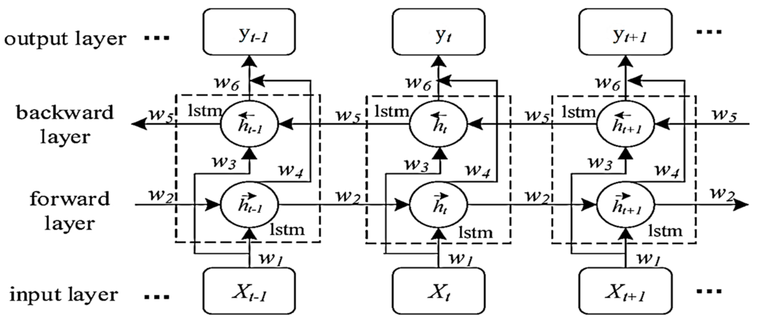
BI-LSTM is developed using the approach of LSTM [49] to increase the classification process performance. BI-LSTM is created by combining RNNs with LSTM approaches (see Figure 7), which can access a long-range context [50]. BI-LSTM networks outperform unidirectional networks, such as LSTM, and they are significantly faster and more accurate than both conventional RNNs and time-windowed multilayer perceptrons (MLPs). Moreover, BI-LSTM has comprehensive detail for the sequential information for all the stages before and after each step in the given sequence [50]. In addition, BI-LSTM employs the LSTM algorithm to compute the hidden layers. Unlike LSTM, a characteristic of BI-LSTM is that it is capable of processing data in two different directions by utilizing two hidden layers and forwarding the results to the same output layer [51,52].
The forward hidden and the backward hidden layers are the main parameters of BI-LSTM, presented in Equations (9) and (10), respectively. Equation (11) represents a combination of the forward hidden and the backward hidden layers. Backpropagation over time is employed to learn the parameters from the training data, using the output sequence to iterate the backward layers based on the error function. The hidden layers (Ң) are used for N stack layers, and the hidden vector series is computed sequentially via n (n = 1) to N (t = 1,…, T), as indicated in Equation (12). In addition, . denotes the network’s ultimate output, as illustrated in Equation (13).
3.4. Study Area and Historical Data Collection
In this study, Dumat al-Jandal City in Al-Jouf province was identified as a case study. Dumat al-Jandal is situated at 29°48′41′′ N latitude, and 39°52′06′′ E longitude, in northwest Saudi Arabia. In 2019, a 400 MW onshore wind farm power plant was constructed in Dumat Al-Jandal City, which is the first and largest regional utility-scale wind power source project in Saudi Arabia. The historical data were collected from the Meteoblue weather service’s portal [54] for Dumat al-Jandal City, which consists of the GHI, DNI, DHI, wind speeds (m/s) at 80 m height, and ambient temperature (°C) at 2 m height, as presented in Figure 8, Figure 9, Figure 10, Figure 11, Figure 12, Figure 13, Figure 14, Figure 15 and Figure 16. The actual historical data covers over 36 years, as hourly intervals, for the period from 1 January 1985 to 26 June 2021, and were used to evaluate and predict the behavior of the GHI, DNI, DHI, wind speed, and ambient temperature for the next 169 h in the future. The geological conditions have changed and varied over the previous 36 years. This large quantity of historical data can provide details that the BI-LSTM neural network prediction model can accurately reflect. The data were analyzed, verified, and cleaned to ensure that no values were missing or duplicated. Moreover, the Dickey–Fuller theory confirmed that all the data were stationary (p-values < 0.05). The p-values were less than 0.05, and the p-value hypothesis was tested. Furthermore, the quality of the historical data was a key element, allowing the BI-LSTM model to extract the essential components and produce accurate results.
3.5. Experimental Setup and Model Configuration
The prediction model was built using Python programming, which has a large memory and can handle enormous quantities of datasets, including a wide range of pre-built libraries. The datasets were prepared and cleaned in preparation for processing. Moreover, a BI-LSTM model was developed, based on computational approaches (Section 3.1, Section 3.2 and Section 3.3), using various layer numbers and model parameters. The numbers of layers, the setting of the neurons, and the training, test, and validation split size are presented in Table 1. Moreover, each type of data required different parameter settings to optimize the BI-LSTM fit owing to the dataset’s size and nature. Furthermore, in the factorization of the learning machine network, the two most essential BI-LSTM model parameters are the number of inputs and the number of neurons in the hidden layer. The error metrics remain nearly constant, with very minor fluctuations when the number of neurons is more than 150 and smaller than 300, which is a result of the extreme learning machine networks’ randomization of input weight. Figure 17 shows the flowchart of the proposed BI-LSTM model.
3.6. The Error Indices
Several indices were specified as popular error metrics to enable the rigorous evaluation of the prediction performance of the two proposed modes. The modeling error indicators were utilized to examine the accuracy of the BI-LSTM model, including the mean square error (MSE), root mean square error (RMSE), the mean absolute percentage error (MAPE), and the mean absolute error (MAE), as presented mathematically in Equations (14)–(18). The (represents the real value, indicates the forecasting observation, and (denotes the number of samples used for the investigation. Moreover, the standard deviation of the residuals (prediction error) is denoted by the abbreviation RMSE, which is the square root of the mean square errors and is considered an effective general purpose error index for numerical forecasts. The best model obtains an MAE value around zero, which is the average error between the actual and predicted variables. The mean squared difference between the estimated and original parameters is simply averaged by MSE, and MAPE calculates the range of error as a percentage. In addition, R-squared (R2) is a statistical index that refers to how much of a dependent variable’s variation is explained by an independent variable, or it is the square of the correlation. In Equation (18), the sum of the square’s residuals is , and the () represents the absolute squares’ number, which is proportional to the data variance.
4. Results and Discussion
The developed BI-LSTM model was implemented to predict the future values of solar irradiance, wind speed, and ambient temperature for 169 h ahead, from 23:00 27 June 2021 to 23:00 3 July 2021, based on the historical dataset covering activity for 36 years in Dumat al-Jandal City. On the basis of the predicted results for solar irradiance, shown in Figure 18, Figure 19, Figure 20, Figure 21 and Figure 22, the BI-LSTM model effectively handled the three different types of irradiances as a multimodal dataset. The GHI (Figure 18a), the DNI (Figure 19a), and the DHI (Figure 20a) did not record any major overfitting between both the experimental and predicted results, which means the BI-LSTM model shows promising performance with this type of dataset. Furthermore, in terms of the accuracy indicators, the BI-LSTM model achieved notable error metrics, as presented in Table 2. The error metrics of GHI were as follows: The RMSE was 7.8 W/m2; the MAE was 5 W/m2; the MSE was 61 W/m2; and the MAPE was 2.5%. In addition, the MAE of GHI was 61 W/m2, which is a high value, with an R2 of 99%. The RMSE of DNI was reduced to 7 W/m2, while the MAE increased to 5.8 W/m2, due to two main factors: (i) the type of dataset; and (ii) the different parameter settings in Table 1. In addition, the MSE of DNI was reduced to 53 W/m2, while the MAPE value grew rapidly to 45% with an R2 of 99%. The MAPE values were affected by the zero values of solar irradiance during the night in historical data. Moreover, the error metrics of DHI recorded a sharp decrease, with an RMSE value of 1.7 W/m2, while the MAE was 1.4 W/m2, the MSE was 3 W/m2, and the MAPE value was reduced to 30% with an R2 of 99%. The DHI’s error metric values were notable compared to the GHI and DNI error values. Figure 18b, Figure 19b and Figure 20b illustrate the future predicted values of the GHI, DHI, and DNI for 169 h ahead. The performance comparison between the proposed BI-LSTM model and the other external solar irradiance models (Table 3) also revealed that the proposed model’s evaluation metrics were superior to those of the other external solar irradiance models.
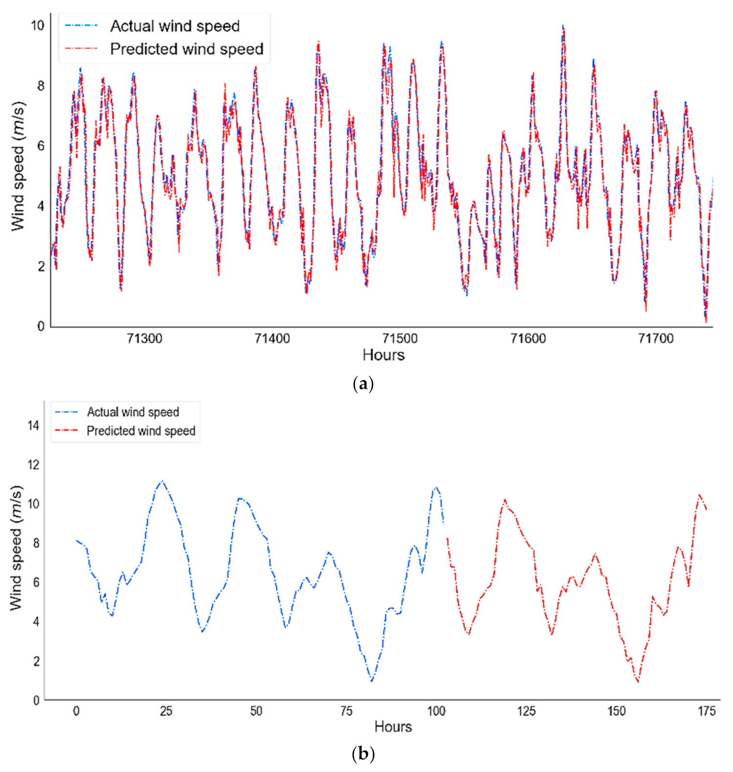
The BI-LSTM model showed remarkable outcomes and performance with the short-term wind speed prediction values, as illustrated in Figure 21. Despite the massive quantity of training data, the BI-LSTM model did not demonstrate overfitting, as seen in Figure 21a. Furthermore, the wind speed values for the next 169 h, from 23:00 27 June 2021 to 23:00 3 July 2021, were forecasted with substantial error metrics, as shown in Figure 21b. The wind speed’s error indicators were as follows: The RMSE was 0.6 W/m2; the MAE was 0.4 W/m2; the MSE was 0.4 W/m2; and the MAPE was 15%. It is clear that all the error metrics, except the MAPE value, decreased with the historical wind speed dataset values, compared to the other types of historical datasets, because of the nature and type of the historical wind speed dataset. The R2 was reduced to 93%; however, the R2 showed notable and agreeable correlation between the variables’ variation of wind speed values. Furthermore, as demonstrated in Figure 22a, the BI-LSTM performed admirably for both the training and test predicted values for ambient temperature. The evaluation metrics of the predicted values for ambient temperature were as follows: The RMSE was 1 W/m2; the MAE was 0.9 W/m2; and the MSE was 1 W/m2. In addition, compared to the wind speed, the MAPE was reduced to 3%, and the R2 increased to 98%, which reflects the high performance of the BI-LSTM model with this type of historical dataset. However, all the error values of the BI-LSTM model with these different types of historical datasets were considered to be relatively small values when compared to other prediction models, demonstrating their flexibility in new historical data observations. Figure 22b presents the predicted values of the ambient temperature for the next 169 h.
The BI-LSTM prediction model was evaluated by implementing the five main types of historical datasets, which are the three types of solar irradiance, wind speed, and the ambient temperature, based on the parameter settings in Table 1. In addition, the proposed BI-LSTM model was compared with several external ANN prediction models to evaluate its performance, as presented in Table 3, Table 4 and Table 5. In comparison to the observational results and ANN models, the BI-LSTM had significant achievements compared to the other models in terms of accuracy and interpretability. The BI-LSTM prediction model showed admirable performance with all three main types of historical datasets, especially for the wind speed and ambient temperature values. The epoch numbers and error indicators had a significant connection, implying that as the epoch numbers rose, the error values would certainly decrease, but the training time would increase. Moreover, by combining a large amount of historical data with a significant amount of training data, the duration of the simulation periods was extended even further. The subsequent steps are reliant on the preceding stages, so the BI-LSTM prediction model must be handled sequentially. Nevertheless, one of the most challenging problems was enhancing this model’s generalization capabilities and achieving improved outcomes. Generalizability is defined as the variation in the recognition rate of the BI-LSTM model when comparing earlier observational datasets (training data) with a dataset that the model has not previously seen (testing data). Furthermore, the lack of generalization of the model leads to the excessive overfitting of training and testing datasets. The BI-LSTM model processes the dataset in two directions, with two hidden layers that feed the data forward to the same output layer. In addition, the BI-LSTM model employs a time series to enhance the generalization ability by taking into consideration the impacts of features on the predicted historical dataset values of the upcoming instant. The BI-LSTM model can be configured to predict the next 1 h in the future, or 24 h ahead, and up to 4 weeks in the future, but increasing the future predicted interval values would raise the error metric indicators. Whenever a sufficient number of historical datasets are chosen, the effectiveness of the BI-LSTM model becomes apparent, and the short-term predictive performance and accuracy are improved.
5. Conclusions
This study contributes to knowledge gaps in renewable energy (wind and solar) short-term forecasting by considering the impacts of solar irradiance and wind speed fluctuation, uncertainty, and intermittence issues, along with the ambient temperatures that affect the power system stability. The scheduling and operation of wind and solar energy integration power systems would be greatly influenced by improving the quality of wind and solar energy predictions. A proposed deep-learning BI-LSTM prediction model based on an RNN time series was trained and validated through a set of selected features, including the algorithms’ neural connection strength, gated units, and layers, which are the best prediction sequence processes for the future performance of solar irradiance, wind speed, and ambient temperature values. The BI-LSTM prediction model was examined and evaluated by implementing five different types of historical datasets, including three types, namely, solar irradiance, wind speed, and the ambient temperature values. In addition, a historical dataset (1 January 1985 to 26 June 2021) was collected from Dumat Al-Jandal City in Saudi Arabia as hourly interval data to predict the next 169 h in the future. The BI-LSTM prediction model proved its ability and capability to handle different types of historical datasets.
The efficacy of the proposed model was evaluated in terms of the performance of the error indexes, such as the RMSE, MAE, MSE, and MAPE values with R2, as summarized in Table 2. The highest RMSE value of the three types of solar irradiance (GHI, DNI, and DHI) was 7.8 W/m2, and the smallest value was 1.7 W/m2, while the greatest value of the MAE was 5.8 W/m2, and the lowest was 1.4 W/m2. Moreover, the MSE value recorded 61 W/m2 as its highest value, and 3 W/m2 as its smallest value. The MAPE values alternated between 45% and 2.5%. The R2 value for all three types of solar irradiance was 99%. The proposed BI-LSTM model produced notable error metric values, such as RMSE, MAE, MSE, and MAPE, which were 0.6, 0.4, and 0.4 m/s and 15%, respectively, for the wind speed values, and 1, 0.9, 0.3 °C, and 3%, respectively, for the ambient temperature. The R2 values for the wind speed and ambient temperature were 93% and 98%, respectively. In addition, the results indicate that the proposed BI-LSTM model had a substantial edge over its competitors in terms of the prediction accuracy, overfitting, minimization of redundancies and training, and testing execution time, and it demonstrated significant performance. These results were supported by the comparison of the proposed BI-LSTM model with the external ANN prediction models, as shown in Table 3, Table 4 and Table 5. Nevertheless, the BI-LSTM model can be upgraded, and the error indicators can be minimized by upgrading the learning performance, optimizing the hidden layers, and modifying the epoch size or learning iterations.
Finally, future work in this field will focus on new short-term forecasting models to forecast wind speeds using various sizes of intervals of historical data and different regions, including solar irradiance.
Author Contributions
F.R.A. wrote most of this paper, including the review of previous research, developed the model, collected data for this research, conducted simulation and analysis, and wrote the original draft of the manuscript. D.C. supervised this research, enhanced the quality of the work, and reviewed the final draft of the article. Both authors have read and agreed to the published version of the manuscript.
Funding
This research received no external funding.
Institutional Review Board Statement
Not applicable.
Informed Consent Statement
Not applicable.
Data Availability Statement
Not applicable.
Conflicts of Interest
The authors declare no conflict of interest.
References
- Ahmad, T.; Chen, H. Deep learning for multi-scale smart energy forecasting. Energy 2019, 175, 98–112. [Google Scholar] [CrossRef]
- Wang, H.; Lei, Z.; Zhang, X.; Zhou, B.; Peng, J. A review of deep learning for renewable energy forecasting. Energy Convers. Manag. 2019, 198, 111799. [Google Scholar] [CrossRef]
- Brownlee, J. Deep Learning for Time Series Forecasting: Predict the Future with MLPs, CNNs and LSTMs in Python; Machine Learning Mastery: San Francisco, CA, USA, 2018; p. 574. [Google Scholar]
- Netzer, Y.; Wang, T.; Coates, A.; Bissacco, A.; Wu, B.; Ng, A.Y. Reading Digits in Natural Images with Unsupervised Feature Learning; Google Research: Mountain View, CA, USA, 2011; p. 9. [Google Scholar]
- Zhao, R.; Yan, R.; Chen, Z.; Mao, K.; Wang, P.; Gao, R.X. Deep learning and its applications to machine health monitoring. Mech. Syst. Signal Process. 2019, 115, 213–237. [Google Scholar] [CrossRef]
- Vincent, P.; Larochelle, H.; Bengio, Y.; Manzagol, P.-A. Extracting and composing robust features with denoising autoencoders. In Proceedings of the ICML′08, 25th international conference on Machine learning, Helsinki, Finland, 5–9 July 2008; pp. 1096–1103. [Google Scholar]
- Hinton, G.E.; Osindero, S.; Teh, Y.-W. A fast learning algorithm for deep belief nets. Neural Comput. 2006, 18, 1527–1554. [Google Scholar] [CrossRef] [PubMed]
- Salakhutdinov, R.; Hinton, G. Deep Boltzmann Machines; University of Toronto: Toronto, ON, Canada, 2009; pp. 448–455. [Google Scholar]
- Sermanet, P.; Chintala, S.; LeCun, Y. Convolutional neural networks applied to house numbers digit classification. In Proceedings of the 21st International Conference on Pattern Recognition (ICPR2012), Tsukuba, Japan, 11–15 November 2012; pp. 3288–3291. [Google Scholar]
- Funahashi, K.-i.; Nakamura, Y. Approximation of dynamical systems by continuous time recurrent neural networks. Neural Netw. 1993, 6, 801–806. [Google Scholar] [CrossRef]
- Wang, H.; Yi, H.; Peng, J.; Wang, G.; Liu, Y.; Jiang, H.; Liu, W. Deterministic and probabilistic forecasting of photovoltaic power based on deep convolutional neural network. Energy Convers. Manag. 2017, 153, 409–422. [Google Scholar] [CrossRef]
- Di Piazza, A.; Di Piazza, M.C.; Vitale, G. Solar and wind forecasting by NARX neural networks. Renew. Energy Environ. Sustain. 2016, 1, 39. [Google Scholar] [CrossRef] [Green Version]
- Wang, F.; Mi, Z.; Su, S.; Zhao, H. Short-term solar irradiance forecasting model based on artificial neural network using statistical feature parameters. Energies 2012, 5, 1355–1370. [Google Scholar] [CrossRef] [Green Version]
- Sözen, A.; Arcaklioğlu, E.; Özalp, M. Estimation of solar potential in Turkey by artificial neural networks using meteorological and geographical data. Energy Convers. Manag. 2004, 45, 3033–3052. [Google Scholar] [CrossRef]
- Altan, A.; Karasu, S.; Zio, E. A new hybrid model for wind speed forecasting combining long short-term memory neural network, decomposition methods and grey wolf optimizer. Appl. Soft Comput. 2021, 100, 106996. [Google Scholar] [CrossRef]
- Hu, Y.-L.; Chen, L. A nonlinear hybrid wind speed forecasting model using LSTM network, hysteretic ELM and Differential Evolution algorithm. Energy Convers. Manag. 2018, 173, 123–142. [Google Scholar] [CrossRef]
- Abayomi-Alli, A.; Odusami, M.O.; Abayomi-Alli, O.; Misra, S.; Ibeh, G.F. Long short-term memory model for time series prediction and forecast of solar radiation and other weather parameters. In Proceedings of the 2019 19th International Conference on Computational Science and Its Applications (ICCSA), Saint Petersburg, Russia, 1–4 July 2019; pp. 82–92. [Google Scholar]
- Liu, X.; Lin, Z. Impact of COVID-19 pandemic on electricity demand in the UK based on multivariate time series forecasting with bidirectional long short term memory. Energy 2021, 227, 120455. [Google Scholar] [CrossRef]
- Jaseena, K.U.; Kovoor, B.C. EEMD-based Wind Speed Forecasting system using Bidirectional LSTM networks. In Proceedings of the 2021 International Conference on Computer Communication and Informatics (ICCCI), Coimbatore, India, 27–29 January 2021; pp. 1–9. [Google Scholar]
- Zhen, H.; Niu, D.; Wang, K.; Shi, Y.; Ji, Z.; Xu, X. Photovoltaic power forecasting based on GA improved Bi-LSTM in microgrid without meteorological information. Energy 2021, 231, 120908. [Google Scholar] [CrossRef]
- Agatonovic-Kustrin, S.; Beresford, R. Basic concepts of artificial neural network (ANN) modeling and its application in pharmaceutical research. J. Pharm. Biomed. Anal. 2000, 22, 717–727. [Google Scholar] [CrossRef]
- Zhang, G.; Patuwo, B.E.; Hu, M.Y. Forecasting with artificial neural networks: The state of the art. Int. J. Forecast. 1998, 14, 35–62. [Google Scholar] [CrossRef]
- van Klompenburg, T.; Kassahun, A.; Catal, C. Crop yield prediction using machine learning: A systematic literature review. Comput. Electron. Agric. 2020, 177, 105709. [Google Scholar] [CrossRef]
- Goodfellow, I.; Bengio, Y.; Courville, A. Deep Learning; MIT Press: Cambridge, UK, 2016; Volume 1. [Google Scholar]
- Almalaq, A.; Edwards, G. A review of deep learning methods applied on load forecasting. In Proceedings of the 2017 16th IEEE International Conference on Machine Learning and Applications (ICMLA), Cancun, Mexico, 18–21 December 2017; pp. 511–516. [Google Scholar]
- Saha, M.; Santara, A.; Mitra, P.; Chakraborty, A.; Nanjundiah, R.S. Prediction of the Indian summer monsoon using a stacked autoencoder and ensemble regression model. Int. J. Forecast. 2020, 37, 58–71. [Google Scholar] [CrossRef]
- Saeed, A.; Li, C.; Danish, M.; Rubaiee, S.; Tang, G.; Gan, Z.; Ahmed, A. Hybrid Bidirectional LSTM Model for Short-Term Wind Speed Interval Prediction. IEEE Access 2020, 8, 182283–182294. [Google Scholar] [CrossRef]
- Wang, H.Z.; Wang, G.B.; Li, G.Q.; Peng, J.C.; Liu, Y.T. Deep belief network based deterministic and probabilistic wind speed forecasting approach. Appl. Energy 2016, 182, 80–93. [Google Scholar] [CrossRef]
- Yan, X.; Liu, Y.; Jia, M. Multiscale cascading deep belief network for fault identification of rotating machinery under various working conditions. Knowl. Based Syst. 2020, 193, 105484. [Google Scholar] [CrossRef]
- Qiu, X.; Zhang, L.; Ren, Y.; Suganthan, P.N.; Amaratunga, G. Ensemble deep learning for regression and time series forecasting. In Proceedings of the 2014 IEEE Symposium on Computational Intelligence in Ensemble Learning (CIEL), Orlando, FL, USA, 9–12 December 2014; pp. 1–6. [Google Scholar]
- Ryu, S.; Noh, J.; Kim, H. Deep neural network based demand side short term load forecasting. Energies 2017, 10, 3. [Google Scholar] [CrossRef]
- Gensler, A.; Henze, J.; Sick, B.; Raabe, N. Deep Learning for solar power forecasting—An approach using AutoEncoder and LSTM Neural Networks. In Proceedings of the 2016 IEEE International Conference on Systems, Man, and Cybernetics (SMC), Budapest, Hungary, 9–12 October 2016; pp. 002858–002865. [Google Scholar]
- Hinton, G.E. A practical guide to training restricted Boltzmann machines. In Neural Networks: Tricks of the Trade; Springer: Berlin/Heidelberg, Germany, 2012; pp. 599–619. [Google Scholar]
- Wu, J.; Mazur, T.R.; Ruan, S.; Lian, C.; Daniel, N.; Lashmett, H.; Ochoa, L.; Zoberi, I.; Anastasio, M.A.; Gach, H.M. A deep Boltzmann machine-driven level set method for heart motion tracking using cine MRI images. Med Image Anal. 2018, 47, 68–80. [Google Scholar] [CrossRef]
- Brownlee, J. Deep Learning with Python: Develop Deep Learning Models on Theano and Tensorflow Using Keras; Machine Learning Mastery: San Francisco, CA, USA, 2016; p. 266. [Google Scholar]
- Brownlee, J. Deep Learning for Computer Vision: Image Classification, Object Detection, and Face Recognition in Python; Machine Learning Mastery: San Francisco, CA, USA, 2019; p. 563. [Google Scholar]
- Baillargeon, J.-T.; Lamontagne, L.; Marceau, E. Mining Actuarial Risk Predictors in Accident Descriptions Using Recurrent Neural Networks. Risks 2021, 9, 7. [Google Scholar] [CrossRef]
- Yin, C.; Zhu, Y.; Fei, J.; He, X. A deep learning approach for intrusion detection using recurrent neural networks. IEEE Access 2017, 5, 21954–21961. [Google Scholar] [CrossRef]
- Pai, P.-F.; Hong, W.-C. Support vector machines with simulated annealing algorithms in electricity load forecasting. Energy Convers. Manag. 2005, 46, 2669–2688. [Google Scholar] [CrossRef]
- Marino, D.L.; Amarasinghe, K.; Manic, M. Building energy load forecasting using deep neural networks. In Proceedings of the IECON 2016—42nd Annual Conference of the IEEE Industrial Electronics Society, Florence, Italy, 23–26 October 2016; pp. 7046–7051. [Google Scholar]
- Chen, L.; Xu, G.; Zhang, S.; Yan, W.; Wu, Q. Health indicator construction of machinery based on end-to-end trainable convolution recurrent neural networks. J. Manuf. Syst. 2020, 54, 1–11. [Google Scholar] [CrossRef]
- Shi, H.; Xu, M.; Li, R. Deep learning for household load forecasting—A novel pooling deep RNN. IEEE Trans. Smart Grid 2017, 9, 5271–5280. [Google Scholar] [CrossRef]
- Liu, Y.; Guan, L.; Hou, C.; Han, H.; Liu, Z.; Sun, Y.; Zheng, M. Wind power short-term prediction based on LSTM and discrete wavelet transform. Appl. Sci. 2019, 9, 1108. [Google Scholar] [CrossRef] [Green Version]
- Kratzert, F.; Klotz, D.; Brenner, C.; Schulz, K.; Herrnegger, M. Rainfall–runoff modelling using long short-term memory (LSTM) networks. Hydrol. Earth Syst. Sci. 2018, 22, 6005–6022. [Google Scholar] [CrossRef] [Green Version]
- Graves, A.; Jaitly, N.; Mohamed, A.-R. Hybrid speech recognition with deep bidirectional LSTM. In Proceedings of the 2013 IEEE Workshop on Automatic Speech Recognition and Understanding, Olomouc, Czech Republic, 8–12 December 2013; pp. 273–278. [Google Scholar]
- Hochreiter, S.; Schmidhuber, J. Long short-term memory. Neural Comput. 1997, 9, 1735–1780. [Google Scholar] [CrossRef]
- Zhao, J.; Deng, F.; Cai, Y.; Chen, J. Long short-term memory-Fully connected (LSTM-FC) neural network for PM2.5 concentration prediction. Chemosphere 2019, 220, 486–492. [Google Scholar] [CrossRef]
- Li, X.; Peng, L.; Yao, X.; Cui, S.; Hu, Y.; You, C.; Chi, T. Long short-term memory neural network for air pollutant concentration predictions: Method development and evaluation. Environ. Pollut. 2017, 231, 997–1004. [Google Scholar] [CrossRef]
- He, L.; Jiang, D.; Yang, L.; Pei, E.; Wu, P.; Sahli, H. Multimodal affective dimension prediction using deep bidirectional long short-term memory recurrent neural networks. In Proceedings of the 5th International Workshop on Audio/Visual Emotion Challenge, Brisbane, Australia, 26 October 2015; pp. 73–80. [Google Scholar]
- Graves, A.; Schmidhuber, J. Framewise phoneme classification with bidirectional LSTM and other neural network architectures. Neural Netw. 2005, 18, 602–610. [Google Scholar] [CrossRef] [PubMed]
- Graves, A.; Mohamed, A.-R.; Hinton, G. Speech recognition with deep recurrent neural networks. In Proceedings of the 2013 IEEE International Conference on Acoustics, Speech and Signal Processing, Vancouver, BC, Canada, 26–31 May 2013; pp. 6645–6649. [Google Scholar]
- Schuster, M.; Paliwal, K.K. Bidirectional recurrent neural networks. IEEE Trans. Signal Process. 1997, 45, 2673–2681. [Google Scholar] [CrossRef] [Green Version]
- Yin, J.; Deng, Z.; Ines, A.V.M.; Wu, J.; Rasu, E. Forecast of short-term daily reference evapotranspiration under limited meteorological variables using a hybrid bi-directional long short-term memory model (Bi-LSTM). Agric. Water Manag. 2020, 242, 106386. [Google Scholar] [CrossRef]
- Meteoblue, A.G. Available online: https://www.meteoblue.com/en/historyplus (accessed on 2 December 2020).
- Alharbi, F.R.; Csala, D. Short-Term Solar Irradiance Forecasting Model Based on Bidirectional Long Short-Term Memory Deep Learning. In Proceedings of the 2021 International Conference on Electrical, Communication, and Computer Engineering (ICECCE), Kuala Lumpur, Malaysia, 12–13 June 2021; pp. 1–6. [Google Scholar]
- Justin, D.; Concepcion, R.S.; Calinao, H.A.; Alejandrino, J.; Dadios, E.P.; Sybingco, E. Using Stacked Long Short Term Memory with Principal Component Analysis for Short Term Prediction of Solar Irradiance based on Weather Patterns. In Proceedings of the 2020 IEEE Region 10 Conference (TENCON), Osaka, Japan, 16–19 November 2020; pp. 946–951. [Google Scholar]
- Peng, T.; Zhang, C.; Zhou, J.; Nazir, M.S. An integrated framework of Bi-directional Long-Short Term Memory (BiLSTM) based on sine cosine algorithm for hourly solar radiation forecasting. Energy 2021, 221, 119887. [Google Scholar] [CrossRef]
- Jeong, S.; Park, I.; Kim, H.S.; Song, C.H.; Kim, H.K. Temperature Prediction Based on Bidirectional Long Short-Term Memory and Convolutional Neural Network Combining Observed and Numerical Forecast Data. Sensors 2021, 21, 941. [Google Scholar] [CrossRef] [PubMed]
Figure 1.
Basic components for ANN neuron model. Copyright © 2021 Elsevier [21].
Figure 1.
Basic components for ANN neuron model. Copyright © 2021 Elsevier [21].

Figure 2.
The configuration of the RBM for two layers. Copyright © 2021 Elsevier [29].
Figure 2.
The configuration of the RBM for two layers. Copyright © 2021 Elsevier [29].

Figure 3.
The configuration of the DBN consists of three mains stacked RBMs with an output layer. Copyright © 2021 Elsevier [29].
Figure 3.
The configuration of the DBN consists of three mains stacked RBMs with an output layer. Copyright © 2021 Elsevier [29].

Figure 4.
The configuration of the DBM. Copyright © 2021 Elsevier [34].
Figure 4.
The configuration of the DBM. Copyright © 2021 Elsevier [34].

Figure 5.
The three main layers of a CNN with the softmax layer. Copyright © 2021 Elsevier [5].
Figure 5.
The three main layers of a CNN with the softmax layer. Copyright © 2021 Elsevier [5].

Figure 6.
The LSTM cell unit. Copyright © 2021 Elsevier [48].
Figure 6.
The LSTM cell unit. Copyright © 2021 Elsevier [48].

Figure 7.
The structure of the BI-LSTM unit [53]. Copyright © 2021 Elsevier.
Figure 7.
The structure of the BI-LSTM unit [53]. Copyright © 2021 Elsevier.

Figure 8.
Hourly intervals historical performance of the GHI over 36 years.

Figure 9.
Hourly intervals historical performance of the DNI over 36 years.

Figure 10.
Hourly intervals historical performance of the DHI over 36 years.

Figure 11.
Hourly intervals historical performances of the GHI, DHI, and DNI.

Figure 12.
Hourly intervals historical performances of the GHI, DHI, and DNI.

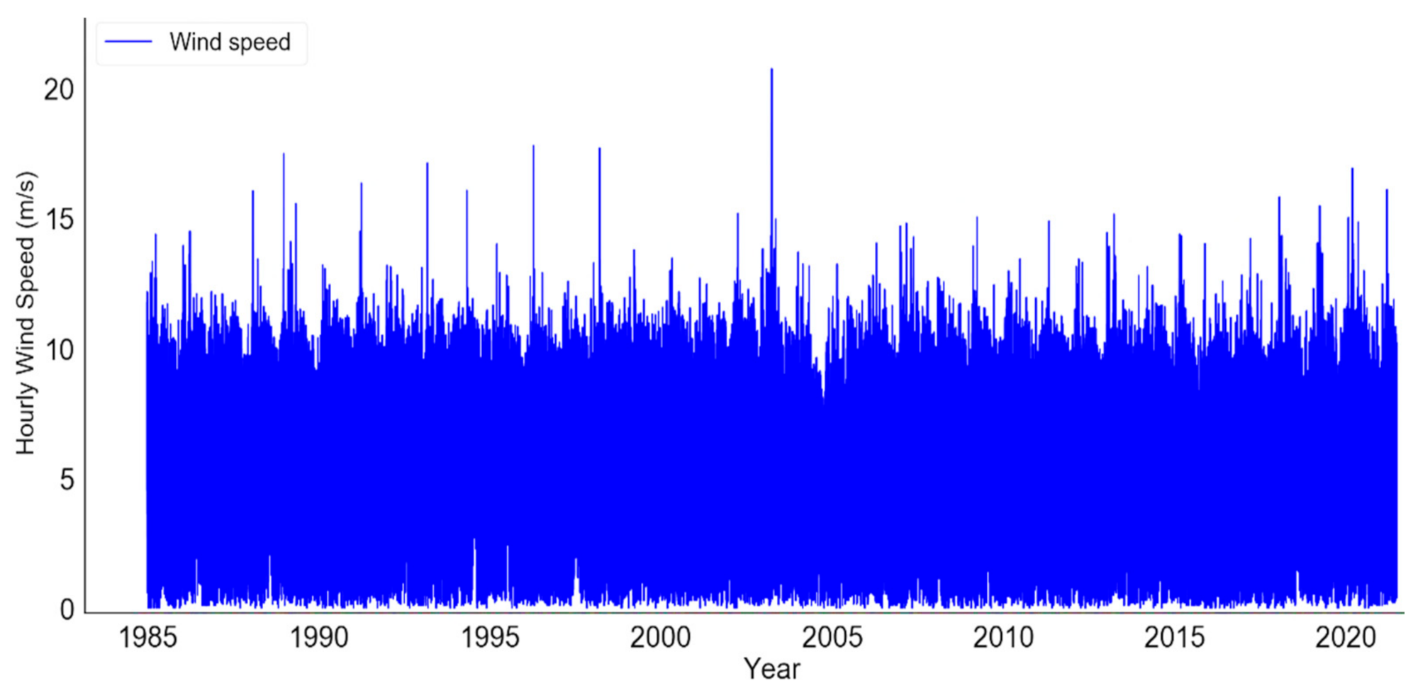
Figure 13.
Hourly intervals historical performance of the wind speed over 36 years.

Figure 14.
Hourly intervals historical performance of the wind speed.

Figure 15.
Hourly intervals historical performance of the temperature.

Figure 16.
Hourly intervals historical performance of the temperature.

Figure 17.
The flowchart of the proposed BI-LSTM model.

Figure 18.
(a) The real and predicted values of GHI, which show the fit and performance of the BI-LSTM model; and (b) the GHI’s predicted future values for the next 169 h.
Figure 18.
(a) The real and predicted values of GHI, which show the fit and performance of the BI-LSTM model; and (b) the GHI’s predicted future values for the next 169 h.

Figure 19.
(a) The real and predicted values of DNI, which show the fit and performance of the BI-LSTM model; and (b) the DNI’s predicted future values for the next 169 h.
Figure 19.
(a) The real and predicted values of DNI, which show the fit and performance of the BI-LSTM model; and (b) the DNI’s predicted future values for the next 169 h.


Figure 20.
(a) The real and predicted values of DHI, which show the fit and performance of the BI-LSTM model; and (b) the DHI’s predicted future values for the next 169 h.
Figure 20.
(a) The real and predicted values of DHI, which show the fit and performance of the BI-LSTM model; and (b) the DHI’s predicted future values for the next 169 h.

Figure 21.
(a) The real and predicted values of wind speed, which show the fit and performance of the BI-LSTM model; and (b) the wind speed’s predicted future values for the next 169 h.
Figure 21.
(a) The real and predicted values of wind speed, which show the fit and performance of the BI-LSTM model; and (b) the wind speed’s predicted future values for the next 169 h.

Figure 22.
(a) The real and predicted values of temperature, which show the fit and performance of the BI-LSTM model; and (b) the temperature’s predicted future values for the next 169 h.
Figure 22.
(a) The real and predicted values of temperature, which show the fit and performance of the BI-LSTM model; and (b) the temperature’s predicted future values for the next 169 h.


Table 1.
Number of layers and the parameter settings of the BI-LSTM model.
| No. | Element | Number of Layers | Size of Layer Neuron | Epoch Size | Batch Size | Validation Split (%) | Training Size (%) | Test Size (%) |
|---|---|---|---|---|---|---|---|---|
| 1 | GHI | 4 | 12 | 30 | 64 | 0.03 | 79 | 20.97 |
| 24 | ||||||||
| 12 | ||||||||
| 6 | ||||||||
| 2 | DNI | 5 | 12 | 50 | 84 | 0.02 | 79 | 20.98 |
| 24 | ||||||||
| 12 | ||||||||
| 12 | ||||||||
| 6 | ||||||||
| 3 | DHI | 2 | 100 | 40 | 74 | 20 | 79 | 20 |
| 50 | ||||||||
| 4 | Wind speed | 2 | 64 | 30 | 64 | 20 | 60 | 20 |
| 1 | ||||||||
| 5 | Temperature | 2 | 64 | 30 | 64 | 20 | 60 | 20 |
| 1 |
Table 2.
The forecasting accuracy indicators for the BI-LSTM model.
| No. | Metric | GHI (W/m2) | DNI (W/m2) | DHI (W/m2) | Wind Speed (m/s) | Temperature (°C) |
|---|---|---|---|---|---|---|
| 1 | RMSE | 7.8 | 7 | 1.7 | 0.6 | 1 |
| 2 | MAE | 5 | 5.8 | 1.4 | 0.4 | 0.9 |
| 3 | MSE | 61 | 53 | 3 | 0.4 | 1 |
| 4 | MAPE (%) | 2.4 | 45 | 30 | 15 | 3 |
| 5 | p-value (%) | 4 × 10⁻²¹ | 3 × 10⁻²³ | 1 × 10⁻²² | 0 | 0 |
| 6 | R2 (%) | 99 | 99 | 99 | 93 | 98 |
Table 3.
Comparison of BI-LSTM proposed model performance with other solar irradiance models.
| No. | Model | RMSE (W/m2) | MSE (W/m2) | MAE (W/m2) | MAPE (%) | R2 (%) |
|---|---|---|---|---|---|---|
| 1 | BI-LSTM [55] | 20.71 | - | 7.60 | 17.40 | 98 |
| 2 | PCA-BILSTM [56] | - | 6063.90 | 42 | - | 94 |
| 3 | SCA-BiLSTM [57] | 119.71 | 69.50 | 79.62 | - | 89 |
| 4 | CEN-BiLSTM [57] | 85.60 | 56 | 66.40 | - | 95 |
| 5 | CEN-SCA-BiLSTM [57] | 81.30 | 52 | 61.80 | - | 95 |
| 6 | BiLSTM [57] | 124 | 70.30 | 82.22 | - | 88 |
| 7 | CEN-ANN [57] | 93.42 | 61 | 71.51 | - | 94 |
| 8 | BI-LSTM proposed model | 5.50 | 39 | 4 | 25 | 99 |
Table 4.
Comparison of BI-LSTM proposed model performance with other wind speed models [16]. Copyright © 2021 Elsevier.
Table 4.
Comparison of BI-LSTM proposed model performance with other wind speed models [16]. Copyright © 2021 Elsevier.
| No. | Model | RMSE (m/s) | MSE (m/s) | MAE (m/s) | MAPE (%) | R2 (%) |
|---|---|---|---|---|---|---|
| 1 | HELM1 | 1.65703 | - | 1.25618 | 21.00415 | 92 |
| 2 | HELM2 | 1.64881 | - | 1.25159 | 20.90677 | 92 |
| 3 | HELM3 | 1.67172 | - | 1.24861 | 20.98445 | 93 |
| 4 | LSTM1 | 1.62832 | - | 1.24653 | 20.76933 | 93 |
| 5 | LSTM2 | 1.62999 | - | 1.21817 | 20.71264 | 93 |
| 6 | LSTM3 | 1.63093 | - | 1.23705 | 20.77809 | 93 |
| 7 | LSTMDE-HELM | 1.59568 | - | 1.20192 | 20.56069 | 93 |
| 8 | BI-LSTM proposed model | 0.6 | 0.4 | 0.4 | 15 | 93 |
Table 5.
Comparison of BI-LSTM proposed model performance with other temperature models [58].
Table 5.
Comparison of BI-LSTM proposed model performance with other temperature models [58].
| No. | Model | RMSE (°C) | MSE (°C) | MAE (°C) | MAPE (%) | R2 (%) |
|---|---|---|---|---|---|---|
| 1 | LSTM | 4.48 | - | 3.49 | - | 89 |
| 2 | BLSTM | 4.42 | - | 3.40 | - | 91 |
| 3 | CNN-BLSTM | 3.98 | - | 3.09 | - | 92 |
| 4 | CNN | 4.77 | - | 3.78 | - | 89 |
| 5 | UM(RDAPS) | 3.74 | - | 2.81 | - | 96 |
| 6 | BI-LSTM proposed model | 1 | 1 | 0.9 | 3 | 98 |
Publisher’s Note: MDPI stays neutral with regard to jurisdictional claims in published maps and institutional affiliations. |
© 2021 by the authors. Licensee MDPI, Basel, Switzerland. This article is an open access article distributed under the terms and conditions of the Creative Commons Attribution (CC BY) license (https://creativecommons.org/licenses/by/4.0/).
Share and Cite
MDPI and ACS Style
Alharbi, F.R.; Csala, D. Wind Speed and Solar Irradiance Prediction Using a Bidirectional Long Short-Term Memory Model Based on Neural Networks. Energies 2021, 14, 6501. https://0-doi-org.brum.beds.ac.uk/10.3390/en14206501
AMA Style
Alharbi FR, Csala D. Wind Speed and Solar Irradiance Prediction Using a Bidirectional Long Short-Term Memory Model Based on Neural Networks. Energies. 2021; 14(20):6501. https://0-doi-org.brum.beds.ac.uk/10.3390/en14206501
Chicago/Turabian StyleAlharbi, Fahad Radhi, and Denes Csala. 2021. "Wind Speed and Solar Irradiance Prediction Using a Bidirectional Long Short-Term Memory Model Based on Neural Networks" Energies 14, no. 20: 6501. https://0-doi-org.brum.beds.ac.uk/10.3390/en14206501
Note that from the first issue of 2016, this journal uses article numbers instead of page numbers. See further details here.