
Effect of Frequency Coupling on Stability Analysis of a Grid-Connected Modular Multilevel Converter System


1
College of Electrical and Information Engineering, Hunan University, Changsha 410000, China
2
Department of Energy Technology, Aalborg University, 9200 Aalborg, Denmark
*
Author to whom correspondence should be addressed.
Energies 2021, 14(20), 6580; https://0-doi-org.brum.beds.ac.uk/10.3390/en14206580
Submission received: 7 September 2021
/
Revised: 8 October 2021
/
Accepted: 9 October 2021
/
Published: 13 October 2021
(This article belongs to the Special Issue Grid Connected Modular Multilevel Converters (MMC) and New Applications)
Abstract
:Due to the internal dynamics of the modular multilevel converter (MMC), the coupling between the positive and negative sequences in impedance, which is defined as frequency coupling, inherently exists in MMC. Ignoring the frequency coupling of the MMC impedance model may lead to inaccurate stability assessment, and thus the multi-input multi-output (MIMO) impedance model has been developed to consider the frequency coupling effect. However, the generalized Nyquist criterion (GNC), which is used for the stability analysis of an MIMO model, is more complicated than the stability analysis method applied on single-input-single-output (SISO) models. Meanwhile, it is not always the case that the SISO model fails in the stability assessment. Therefore, the conditions when the MIMO impedance model needs to be considered in the stability analysis of an MMC system should be analyzed. This paper quantitatively analyzes the effect of frequency coupling on the stability analysis of grid-connected MMC, and clarifies the frequency range and grid conditions that the coupling effect required to be considered in the stability analysis. Based on the quantitative relations between the frequency coupling and the stability analysis of the grid-connected MMC system, a simple and accurate stability analysis method for the grid-connected MMC system is proposed, where the MIMO impedance model is applied when the frequency coupling has a significant effect and the SISO impedance model is used if the frequency coupling is insignificant.
1. Introduction
Due to the modularity, scalability, high efficiency, and superior harmonic performance [1,2,3], modular multilevel converters (MMCs) are increasingly used in high-voltage/high-power applications [4,5], e.g., high-voltage direct current (HVDC) transmission and static synchronous compensation (STATCOM). However, the resonant interactions among the MMCs and electrical systems may result in harmonic instability in these systems [6]. When MMC is connected to a weak grid, the stability margin of the system is significantly reduced, which can easily lead to resonance problems [7,8]. The instability issues in the MMC system have been reported in [9,10]. It is essential that the stability of the grid-connected MMC system is considered.
The impedance-based analysis method is an effective method for assessing the system stability [11], and admittance/impedance modeling is a prerequisite to applying the analysis [12,13]. Since the MMC has become the state-of-the-art technology for high-power applications, the admittance/impedance modeling of MMC has attracted extensive research. The impedance model of an MMC connected to a wind farm is developed in [14], where the internal harmonics of an MMC are included based on the harmonic state-space (HSS) modeling method. The impedance model of a grid-connected MMC is derived in [15,16], where the impedance shaping effect produced by different control schemes was fully elaborated. In the above studies, the admittance/impedance of MMC is seen as the single-input single-output (SISO) form. When the symmetric control is adopted in the two-level voltage source converter (VSC), the decoupled SISO admittance/impedance is considered reasonable in the VSC [17,18]. However, different from the VSC, the coupling between the positive and negative sequences in impedance, i.e., frequency coupling, exists in the MMC even under the symmetric control. As concluded in [19,20], the frequency coupling has an impact on the stability assessment of grid-connected VSC at low frequency. Thus, the frequency coupling of MMC admittance should be considered in the stability assessment of a grid-connected MMC system.
Recently, the frequency coupling of MMC admittance/impedance has received considerable attention [21,22,23,24,25,26,27,28,29]. Two-order MMC impedance matrixes are proposed in [21,22,23,24,25,26], where the off-diagonal elements in the matrix capture the frequency coupling in MMC impedance. A three-order impedance model of MMC is derived in [27], and the impedance model includes the coupling among the positive-sequence system, the negative-sequence system, and the DC system. The authors of [28,29] proposed an equivalent SISO impedance model of grid-connected MMC considering its frequency coupling, and the model shows that the frequency coupling makes the MMC impedance be coupled with the grid impedance.
Previous research has shown that ignoring the frequency coupling may lead to inaccurate stability assessment of the interconnection systems [20,21]. Although the SISO impedance model provides simplicity and convenience for the stability analysis, some cases exist where the SISO impedance model leads to the wrong stability assessment [30]. To include the frequency coupling effect, [21,22,23,24,25,26,27] apply the MIMO impedance model of MMC in the stability analysis of MMC-HVDC, where the generalized Nyquist criterion (GNC) is inevitably introduced in the stability assessment. However, the stability assessment applied by the GNC is more complicated than the SISO analysis tool. Meanwhile, it is not always the case that the SISO model fails in the stability assessment. Therefore, the condition that the frequency coupling must be considered in the stability analysis of grid-connected MMC deserves to be studied.
This paper quantitatively analyzes the effect of frequency coupling on the stability analysis of grid-connected MMC. Based on the amplitude comparison between the sequence impedance and coupling term of the MMC under different control schemes, the frequency range that the coupling should be considered in the stability analysis is given. Furthermore, following the stability assessment procedure of the grid-connected MMC system, the grid conditions when the coupling effect needs to be considered in the stability analysis are defined. Based on the quantitative relations between the frequency coupling and the stability analysis of the grid-connected MMC system, a simple stability analysis method for the grid-connected MMC is proposed without losing accuracy. Specifically, in the cases where the coupling needs to be considered, the stability of MMC should be assessed by the GNC using the MIMO model, while for the other cases, the SISO model can be used.
The paper is organized as follows: The system model of the grid-connected MMC is given in Section 2. Section 3 derives the admittance matrix of MMC considering the frequency coupling, which is validated by experimental measurements. In Section 4, the coupling effect on the stability analysis of grid-connected MMC is analyzed. Section 5 draws the conclusions.
2. System Model
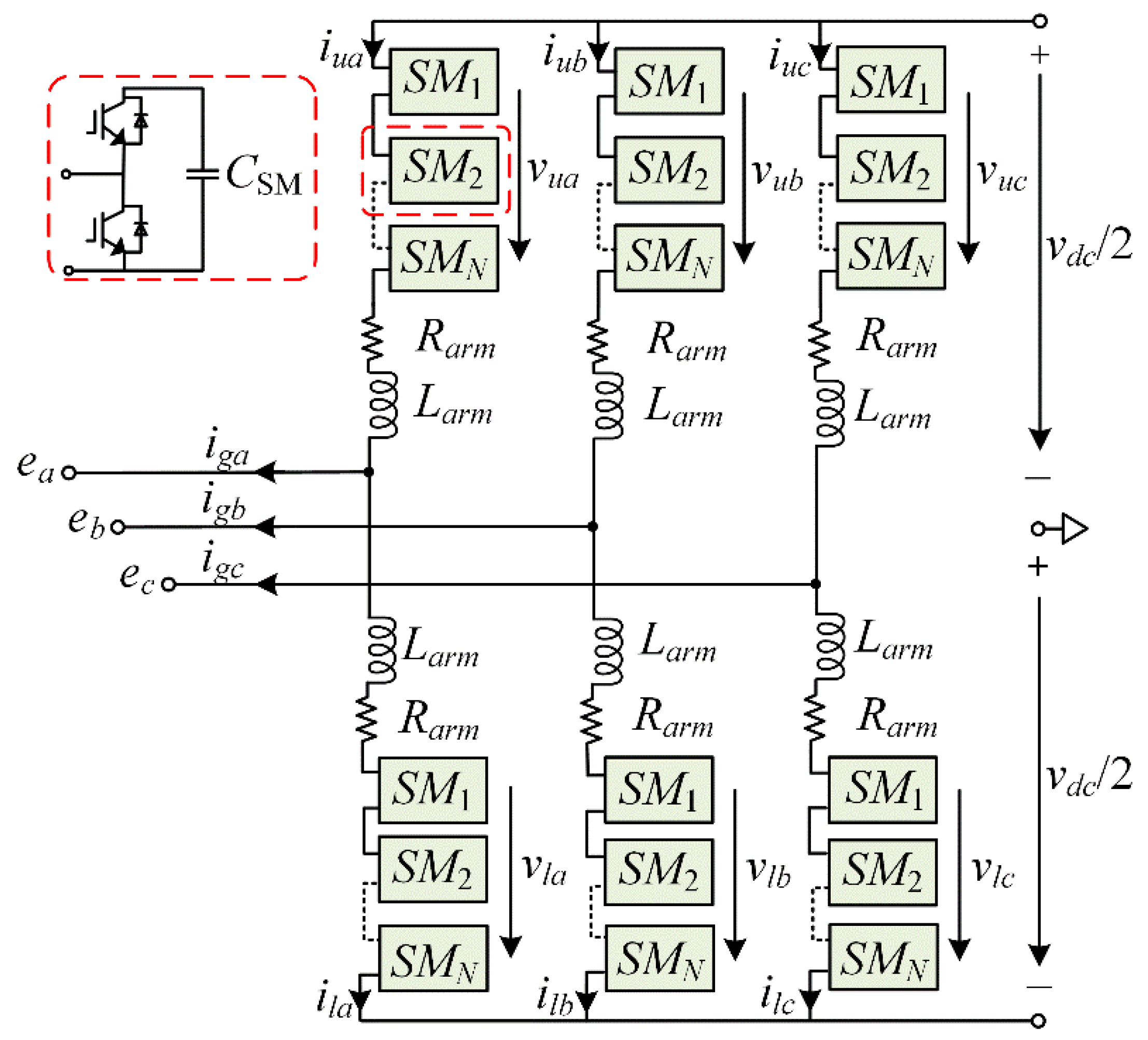
The topology of a three-phase MMC is indicated in Figure 1. Each phase of MMC includes an upper arm and a lower arm, and each arm consists of an N submodule (SM) and arm inductor. Each SM constitutes an IGBT half-bridge and a capacitor CSM.
The MMC is modeled in one phase, for example, which makes the subscript denoting the phase dropped when not needed. The phase current ig and circulating current ic are defined as:
where iu(t) and il(t) are the upper and lower arm currents.
Applying Kirchhoff’s law, the current dynamics can be obtained as:
where vu(t) and vl(t) are the upper and lower arm voltage, e(t) is the point-of-common-coupling (PCC) voltage, and vdc is the DC-bus voltage.
This paper adopts the time-averaged model of MMC, where the switching operations of the SMs are neglected and the SM capacitor voltages are assumed to be balanced [31]. Thus, the individual SMs dynamics in the arm can be neglected. Based on the averaged model, the arm voltages vu,l (t) and the sum capacitor voltages are obtained as:
where Carm = CSM/N is the arm equivalent capacitance, and mu,l(t) are the modulation indices generated by the control scheme of MMC, expressed as:
where vs(t) and vc(t) are the voltages from the phase current controller and circulating current controller, respectively.
Substituting Equations (1) and (4) into Equations (2) and (3) yields:
Equations (5), (7) and (8) represent the dynamic model of MMC.
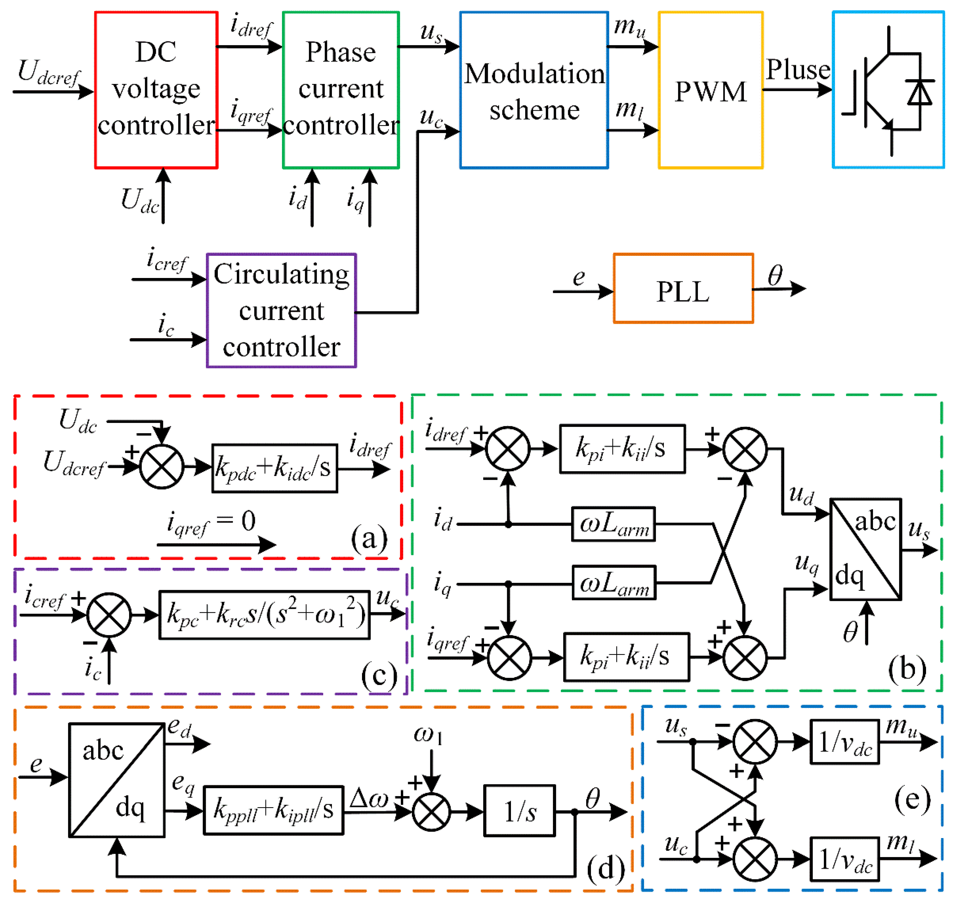
Figure 2 shows the control scheme of the grid-connected MMC. The DC-bus voltage controller adopts the proportional-integral (PI) compensator to keep the DC-bus voltage as a constant and generate the reference current for the current control [32], which is shown in Figure 2a; kpd and kid are the proportional and integral coefficients of the dc voltage controller; the q-axis reference current is set to zero for unity power factor operation. The phase current controller adopts the PI compensator to properly track the reference currents, as illustrated in Figure 2b; kpi and kii are the proportional and integral coefficients of the phase current controller. The circulating current suppression controller (CCSC) using the proportional resonant (PR) controller is shown in Figure 2c, which suppresses the 2nd harmonics in the circulating current [33]; kpc and krc are the proportional and resonant coefficients of the CCSC. The phase-locked loop (PLL) synchronizes the MMC with the grid, as shown in Figure 2d; the proportional and integral coefficients of the PLL are kppll and kipll. The voltages driving the grid current and circulating current (us and uc) are used for computing the modulation indices.
3. Admittance Modeling of MMC Considering Frequency Coupling
3.1. Small-Signal Model of MMC
The AC-side admittance of MMC is obtained by injecting a perturbation voltage ep(t) at an arbitrary perturbation frequency fp in the PCC voltages at a fundamental frequency f1, and calculating the corresponding current. The perturbation voltage is defined as:
where Ep is the magnitude of the perturbation voltage.
Based on the harmonic linearization, the small-signal equations of the MMC in the time-domain are given as:
where the subscript “p” indicates the small-signal variable and the subscript “0” represents the variable at the steady state.
3.2. Frequency Coupling Analysis of MMC Admittance
It is known that the positive-sequence perturbation voltage at fp will lead to the perturbation current at the same frequency in the power converter. As for MMC, the perturbation current at fp will generate perturbation capacitor fluctuation voltage at f1 ± fp due to the multiplication between the modulation index m1 at f1 and the perturbation current at fp, as shown in Equations (12) and (13). Subsequently, the multiplication of at f1 ± fp with m1 at f1 leads to the perturbation arm voltages vp at fp and fp ± 2f1. The perturbation arm voltages finally result in the perturbation arm currents at fp and fp ± 2f1. Similarly, the perturbation modulation index at fp caused by the perturbation current will also generate the perturbation currents at fp and fp ± 2f1. Considering the delay fundamental cycle caused by perturbation voltage ep, the perturbation arm current at fp + 2f1 is a zero-sequence current, which will not appear in the three-phase three-line MMC system.
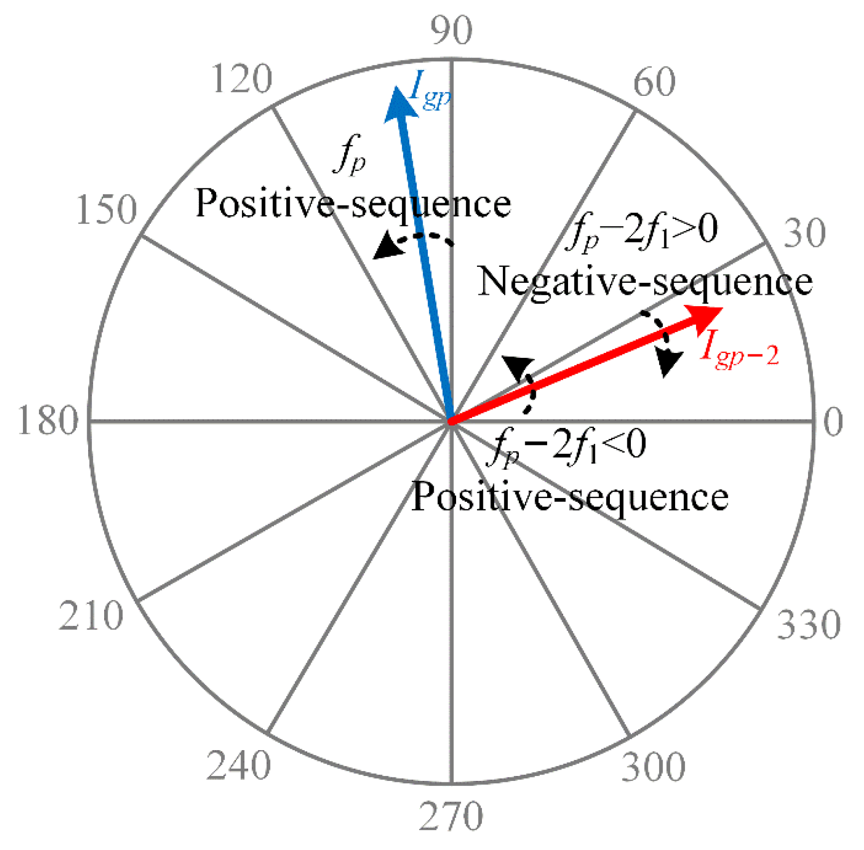
Based on the analysis above, it can be observed that the perturbation voltage at fp will lead to the perturbation currents at fp and fp − 2f1 for the MMC even under the symmetric control. The response of a linear and decoupled system contains only one component with the same frequency corresponding to the perturbation voltage. The additional component indicates the frequency coupling inherently exists in the MMC admittance, where the root cause is the capacitor voltage harmonics in MMC. The illustration of the frequency coupling is shown in Figure 3.
The sequence of the perturbation currents in MMC is shown in Figure 4. For the positive-sequence perturbation voltage at fp, the corresponding current at fp is the positive-sequence component. The perturbation current at fp − 2f1 is yielded due to the capacitor fluctuation voltage in MMC. As can be seen from Figure 4, when the frequency fp is above 2f1, the perturbation current at fp − 2f1 is the negative-sequence component. While, if fp is below 2f1, the perturbation currents at fp − 2f1 is the negative-sequence component at negative frequency, which is equal to the positive-sequence current at positive frequency.
It should be noted that the perturbation voltage at fp will also interact with the state variables at nf1 (n ≥ 3) and generate the perturbation currents at fp ± nf1. However, the amplitude of the perturbation currents is gradually decreased as the frequency increases. As shown in Figure 5, the amplitude of the harmonic currents at fp ± nf1 (n ≥ 3) is much smaller than that of the harmonic current at fp, which can be ignored.
3.3. Admittance Modeling
Due to the MMC internal dynamics, the multiple harmonics must be considered in the admittance modeling of MMC. There are several frequency-domain methods to derive the MMC admittance model (e.g., multiple-harmonic linearization [16,34], HSS modeling [14], harmonic transfer function [23], etc.). The essences of these methods are identical, which can simultaneously represent multiple frequency responses. Similar to these methods, the frequency-domain model of MMC which contains multiple perturbation components at ωp, ωp ± ω1, ωp ± 2ω1, …, ωp ± nω1, is used in this paper.
The perturbation state variables in the time-domain can be expressed in the form of Fourier series as below:
where Xpn represents the Fourier coefficient corresponding to the frequency of ωp ± nω1.
Then, based on the Fourier series and harmonic balance theory [35], the time-domain model of the MMC in Equations (10)–(13) can be transformed to the frequency-domain model, which is expressed as:
where:
Ap and Bp are given in the Appendix A.
It should be noted that the perturbation modulation Mup±n and Mlp±n is related to the control dynamics. Thus, the control model should be obtained to get the admittance model. The detailed derivations of the control modeling are given in Appendix B.
Based on the control modeling in Appendix B, the perturbation modulation indices are expressed as:
Substituting the control model under positive-sequence perturbation voltage into the small-signal model in the frequency-domain, the perturbation state variables can be calculated by:
Extracting the perturbation currents at fp and fp − 2f1 from the perturbation state variables, the positive-sequence admittance and the coupling term of MMC can be calculated as:
Similarly, the negative-sequence admittance and the coupling term of MMC can be calculated by substituting the control model under negative-sequence voltage perturbation into the small-signal model, which is obtained as:
where Ep−2 is the complex phasors of the negative-sequence perturbation voltage at fp − 2f1, and Igp0 is the complex phasors of the perturbation current at fp.
Considering the frequency coupling, the admittance matrix of MMC can be defined as:
where the diagonal elements represent the sequence admittance, whereas the off-diagonal elements represent the coupling terms.
3.4. Experimental Verification
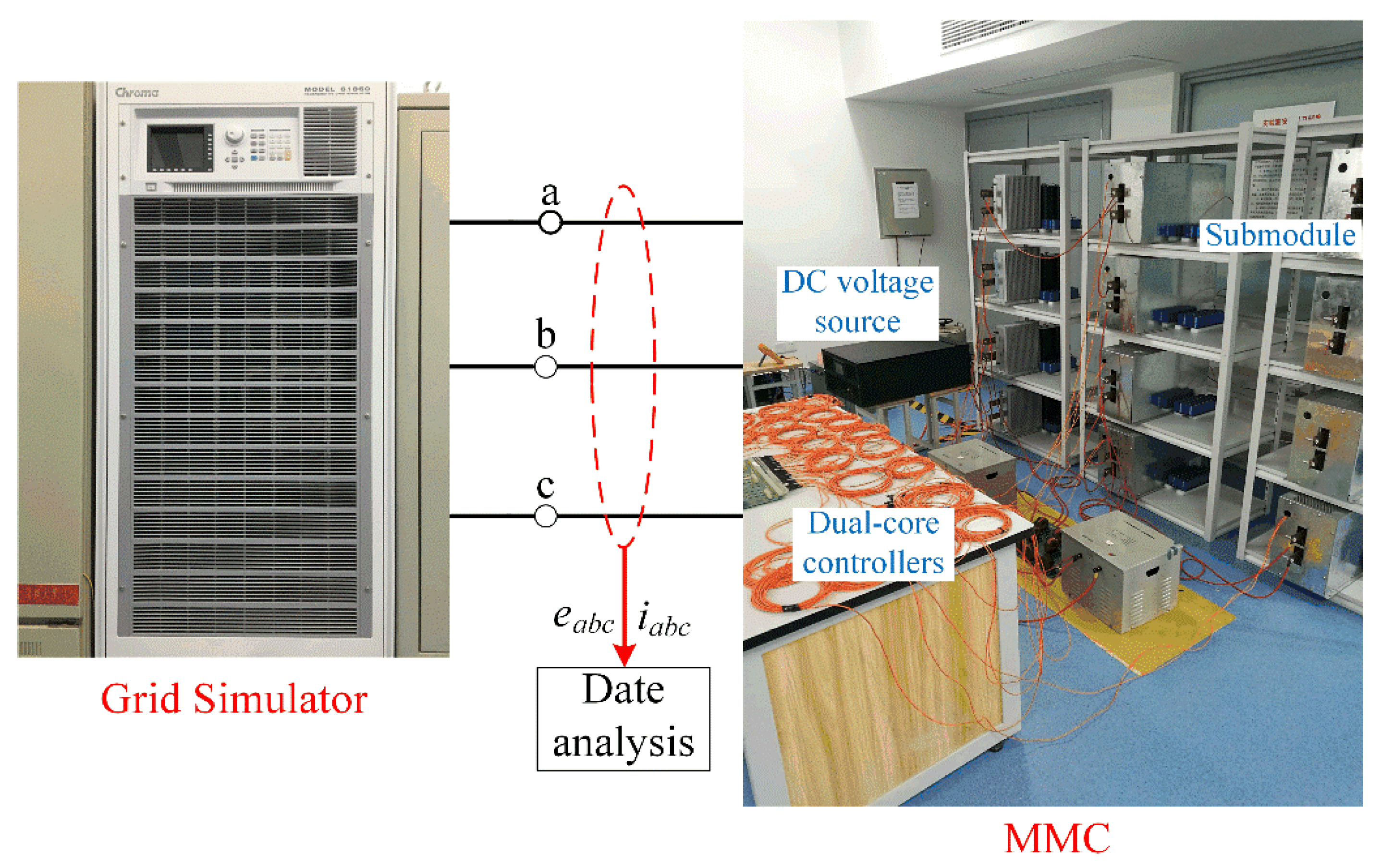
To validate the MMC admittance model, the admittance measurements are carried out on a down-scaled MMC prototype. The main parameters of MMC are listed in Table 1. The configuration and photograph of the experimental setup for measuring the MMC admittance are shown in Figure 6 and Figure 7. The grid simulator, acting as the grid voltage source and the perturbation voltage injection source, injects the perturbation voltages ranging from 1 to 1000 Hz in one-phase (phase b) voltage. Moreover, in order to acquire the components of the admittance matrix in Equation (24), two linearly independent perturbation voltages at fp and fp − 2f1 are required to gain enough information [36]. The perturbation voltage is firstly injected while the perturbation voltage at fp − 2f1 is equal to zero. Similarly, a second perturbation sequence is implemented by injecting the perturbation voltage with the perturbation voltage at fp being zero. Then, the perturbation voltage and resulting current are extracted from the measured voltage and current by FFT. When the perturbation voltage at fp is superposed to the voltage at f1, the response currents at fp and fp − 2f1 are only caused by ep1(fp) and the admittance Yp and Cp−2 are identified as:
Similarly, when the perturbation voltage at fp − 2f1 is injected, the admittance Yn, Cn+2 can also be identified as:
Note that if fp is below 2f1, the perturbation components at fp − 2f1 is the component at positive frequency with the opposite phase angle. The frequency and the phase angle of the perturbation components should be revised; the detailed process of the revision has been described in [37].
Figure 8 shows the comparison between the analytical admittance model and the experimental measurements of the MMC. The sequence analytical admittance models of MMC are denoted by the blue line, and the red line denotes the coupling terms in the MMC admittance matrix model. The measured values are denoted by the dots. The comparison in Figure 8 shows a good agreement between the analytical admittance models and the experimental measurements. This agreement validates the accuracy of the MMC admittance model. It should be noted that the magnitude of coupling terms (blue line) is close to that of sequence admittance (red line) at low frequency. Yet, the magnitudes of coupling terms are much smaller than that of sequence admittance above 100 Hz, which indicates the phenomenon of frequency coupling is not obvious at high frequency.
4. Effect of Frequency Coupling on Stability Analysis of Grid-Connected MMC
Figure 9 shows the small-signal description of the grid-connected MMC system. Assuming the grid is stable without the MMC, and the MMC is stable when connected to an ideal grid, the stability of the grid-connected MMC system can be assessed by the impedance ratio Zg(s)YMMC(s), which should satisfy the Nyquist stability criterion.
Due to the frequency coupling in the MMC admittance, the generalized Nyquist criterion (GNC) should be applied to evaluate the system stability [38]. The grid weakness is distinguished by the short circuit ratio (SCR) as it is an inverse of the grid impedance. In general, SCR ≥ 3 denotes a strong system; 2 ≤ SCR < 3 denotes a weak system; and 1 ≤ SCR < 2 indicates a very weak system [39,40]. Then, the stability can be examined by checking the Nyquist plot of Zg(s)YMMC(s), i.e., λ1, λ2, which are obtained as:
where:
Based on Equation (27), it can be concluded that if the coupling terms are ignored in the stability analysis, a deviation will be generated in the stability assessment, which is calculated as:
According to Equation (29), the deviation Δλ is proportional to the coupling terms. As can be seen from Figure 8, the magnitude of coupling terms is close to that of sequence admittance below 100 Hz, which leads to the relatively high deviation in the stability assessment. Thus, ignoring the frequency coupling has an influence on the stability assessment of grid-connected MMC under low frequency.
The effect of frequency coupling on the stability analysis of grid-connected MMCs can be evaluated following the steps shown in Figure 10. As seen from Figure 10, the SCR is initialized with 0.1. When the coupling is considered, the critical stability point SCR1 increases with a fixed step during every iteration. The critical stability point SCR2 with frequency coupling ignored is obtained in a similar way. Thus, if SCR belongs to [SCR1, SCR2], neglecting the frequency coupling leads to the incorrect stability analysis. If SCR does not belong to [SCR1, SCR2], the same stability analysis can be obtained, even though the frequency coupling is not considered. Based on the above analysis, the effect of frequency coupling on the stability analysis under different grid conditions can be evaluated.
An example MMC in China is analyzed in this paper to account for the coupling effect on the system stability analysis. The parameters of MMC are shown in Table 2. Due to the high power and a large number of submodules in the MMC-HVDC system, the simulation in MATLAB/Simulink is considered to be an acceptable method to verify the system-level stability analysis. Starting from the MMC operated with the phase current controller, the different controller elements are progressively added to analyze the frequency coupling effect on the stability analysis of the MMCs under different control schemes.
4.1. Case of MMC with Phase Current Controller
The Bode diagrams of the sequence admittance and coupling term of the MMC with the phase current controller are shown in Figure 11, where only the magnitude of Yp and Cp−2 are shown. It can be seen that the magnitude of the coupling term is close to that of the sequence admittance under 20 Hz, which indicates that the frequency coupling of MMC has a significant influence on the stability analysis of the grid-connected MMC system under 20 Hz.
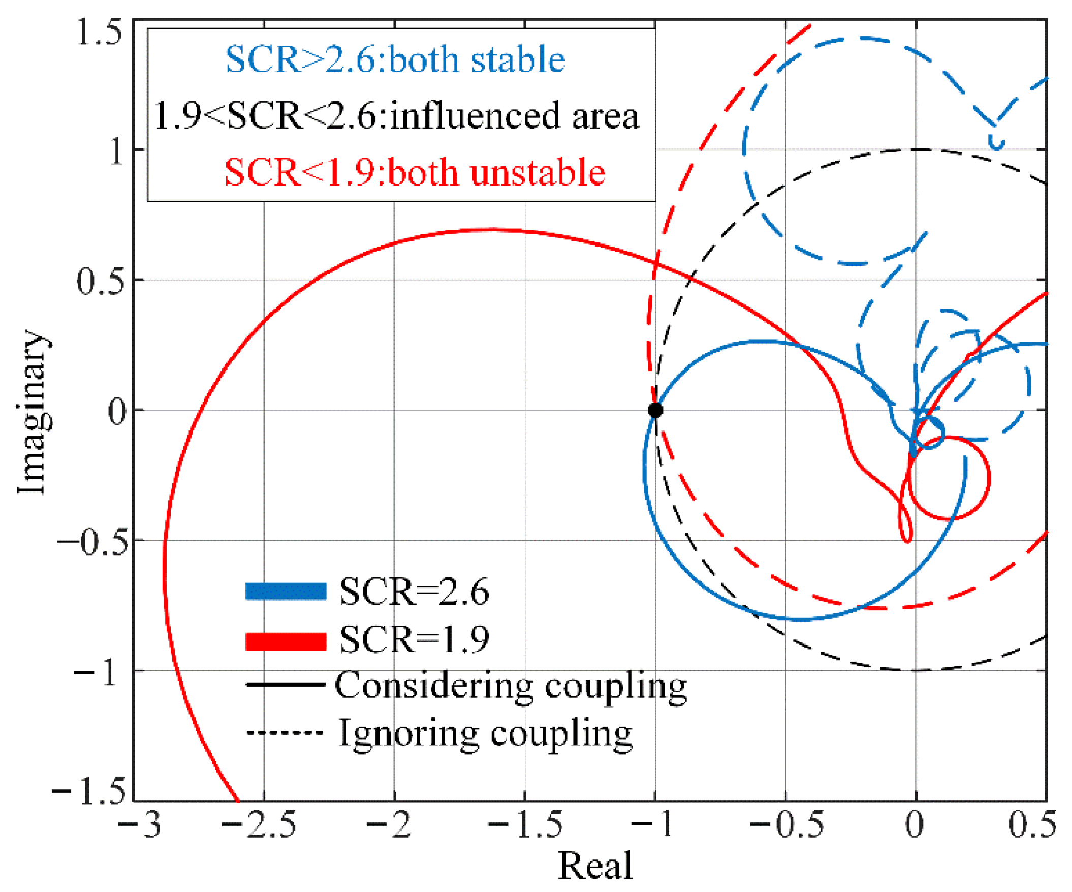
With the iteration shown in Figure 10, the condition for considering the coupling is obtained as 1.9 < SCR < 2.6. Figure 12 shows the Nyquist plot of Zg(s)YMMC(s) considering or ignoring the frequency coupling, where only the dominant eigenvalue (λ1) is shown for simplicity. It can be seen when the coupling is considered, the Nyquist plot encircles the point (−1, j0) under SCR < 2.6, meaning that the system is unstable if SCR < 2.6. However, the Nyquist plot ignoring the coupling does not encircle the point (−1, j0) until SCR is less than 1.9, indicating the system is predicted to be unstable when SCR < 1.9. Therefore, ignoring the coupling will lead to a wrong stability assessment if 1.9 < SCR < 2.6.
Figure 13 shows the time-domain simulation results of the MMC under a step change of the grid condition, where only the phase current controller is adopted. The parameters in the simulation are the same as those in Table 2. It can be seen that the system is stable when SCR = 2.7. However, the grid-connected MMC loses stability as SCR = 2.5, which is consistent with the theoretical analysis in Figure 12. The dominant oscillation frequency is around 18 and 82 Hz. It is the coupling effect that causes both the sub- and super-synchronous frequency in the oscillation.
4.2. Case of MMC with CCSC
For this case, only the phase current controller and CCSC are applied in the control scheme. The Bode diagrams of the sequence admittances and coupling terms of MMC with and without the CCSC are shown in Figure 14 (only magnitude plots are shown). It can be seen that the CCSC can suppress the low-frequency resonance characteristics of both the sequence admittance and the coupling terms of MMC. Yet, the frequency coupling still exists in the MMC admittance, which indicates that the CCSC cannot eliminate the frequency coupling of the MMC system.
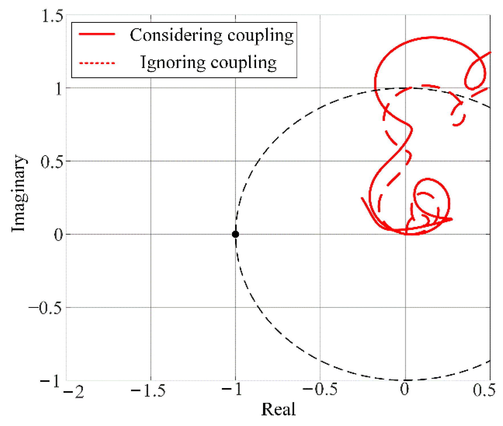
Figure 15 shows the Nyquist plot of Zg(s)YMMC(s) with CCSC, where the SCR = 1.5. As shown in Figure 15, both the stability assessments considering or ignoring the frequency coupling indicate that the system is stable even under the ultra-weak grid. The phenomenon can be explained as follows: As for the MMC with CCSC, the capacitive behavior of MMC impedance caused by its internal dynamics has been suppressed, which makes the stability margin of grid-connected MMCs sufficient even under a very weak grid. For the system with a sufficient stability margin, ignoring the coupling will not lead to a wrong stability assessment. Therefore, for the MMC only with the phase current controller and CCSC, ignoring the frequency coupling will not affect the stability analysis of the grid-connected MMC.
4.3. Case of MMC Considering PLL Dynamics
For this case, the phase current controller, CCSC, and PLL are adopted in MMC. Figure 16 shows the PLL effect on the sequence admittances and coupling terms of MMC. It can be observed that the PLL mostly affects the sequence admittances and coupling terms around the fundamental frequency. Furthermore, it is noted that except for the fundamental frequency, the coupling term at another frequency is barely affected by PLL.
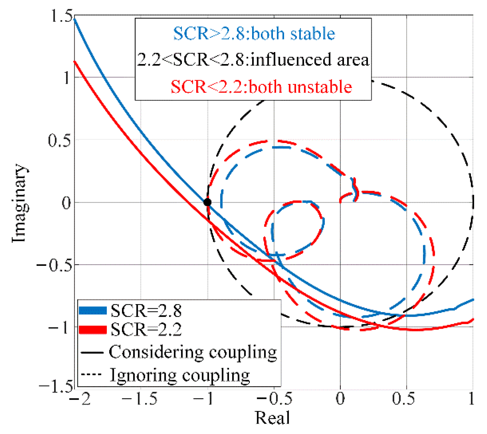
Substituting the MMC admittance model considering PLL dynamics into the iterative procedure in Figure 10, the conditions for considering the frequency coupling can be obtained. The results show that when SCR < 2.2, the stability assessments are unstable regardless of whether the coupling is ignored or considered. In addition, when SCR > 2.8, the system is always stable regardless of whether the coupling is ignored or considered. However, if the frequency coupling is ignored at 2.2 < SCR < 2.8, an inaccurate stability analysis will be obtained. Figure 17 shows the characteristic loci of Zg(s)YMMC(s) with PLL dynamics. The grid condition of 2.2 < SCR < 2.8 is the condition that ignoring the coupling will result in a wrong stability estimation.
Figure 18 shows the time-domain simulation results of the MMC under a step change of the grid condition, where the PLL bandwidth is set as 40 Hz. It can be seen the system loses stability when SCR = 2.7.
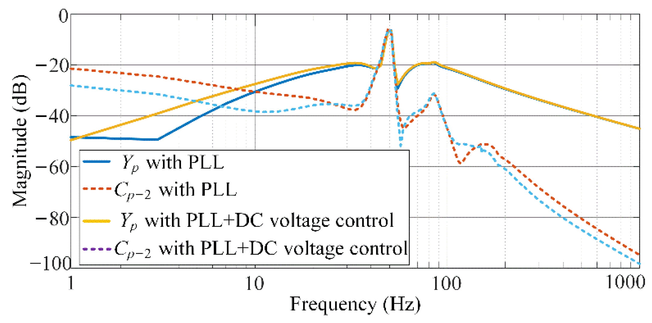
For this case, the DC-voltage control is added in the case of MMC considering PLL dynamics. Figure 19 shows the effect of DC-bus voltage control on the MMC admittance. It can be seen that the DC-bus voltage control mainly affects the admittance responses of MMC below 10 Hz. Considering that adding DC voltage control hardly changes the MMC admittance characteristics, the stability analysis considering voltage control is almost the same as the stability analysis considering PLL dynamics. Therefore, the condition for considering the coupling is the same as that of MMC considering the PLL dynamics, which is not analyzed in detail.
4.4. Discussion
Based on the above analysis, it can be observed that ignoring the frequency coupling of MMC admittance leads to the inaccurate stability conclusion under certain grid conditions. However, it is not always the case that ignoring coupling fails in the stability assessment. The conditions for considering the coupling effect are quantitatively defined in Section 4 (1–4). Table 3 summarizes the conditions for different cases of MMC.
Previous studies have analyzed the stability of an MMC system using the SISO impedance model [14,15]. Yet, the SISO model cannot include the impact of frequency coupling on the stability, which may lead to inaccurate results in some cases. Afterward, the MIMO modeling method, which considers the frequency coupling effect, is proposed. Compared with the SISO model, the MIMO model can guarantee the accuracy of stability analysis results under any circumstances. However, the stability analysis method applying MIMO (e.g., GNC) is more complicated than the stability analysis method applying on the SISO model (e.g., Bode plot). Meanwhile, it is not always the case that the SISO model fails in the stability assessment of the grid-connected MMC. Thus, different models can be applied to the stability of MMCs under different grid conditions, as shown in Figure 20. According to the significance evaluation of frequency coupling and the practical grid condition, it can be determined whether the MIMO model of MMC impedance needs to be applied in the stability assessment. In the cases where the coupling needs to be considered, the stability of MMC should be assessed by the GNC using the MIMO model, while for the other cases, the SISO model can be used. Compared to the stability analysis method that always applies the MIMO model, the proposed method is simpler without losing accuracy.
5. Conclusions
Ignoring the frequency coupling will lead to inaccuracy in stability analysis for the grid-connected MMC under a certain short circuit ratio of the grid. However, it is not always the case that ignoring coupling fails in the stability assessment. In order to clarify the case that the coupling must be considered, the effect of frequency coupling of MMC impedance on the stability analysis of grid-connected MMC was quantitatively analyzed in this paper. On this basis, a stability analysis method was proposed, where GNC is applied when the frequency coupling has a significant effect and the SISO analysis tool (e.g., Bode plot) is used if the coupling is insignificant. Compared to the stability assessment always applying the MIMO model, the proposed method is more simplified without losing accuracy. The grid impedance is different for the grids under different active power. Thus, the grid conditions that the coupling effect needs to be considered in the stability analysis are different for the grids under different active power. The proposed method can be only applied for a grid with a fixed power. The method suitable for the grids under different active power will be studied in the future.
Author Contributions
Conceptualization, Y.W., Q.X.; methodology, Y.W., Q.X.; software, Y.W.; validation, Y.W., Q.X.; formal analysis, Y.W., Q.X.; investigation, Y.W., Q.X.; resources, Q.X.; data curation, Y.W.; writing—original draft preparation, Y.W.; writing—review and editing, Y.W.; visualization, Y.W.; supervision, J.M.G.; project administration, Q.X.; funding acquisition, Q.X. All authors have read and agreed to the published version of the manuscript.
Funding
This research was funded by the National Natural Science Foundation of China (51807056).
Institutional Review Board Statement
Not applicable.
Informed Consent Statement
Not applicable.
Data Availability Statement
Not applicable.
Conflicts of Interest
The authors declare no conflict of interest.
Appendix A
The expression of Ap and Bp:
where I is the identity matrix and O denotes the zero matrix. A and B are the Toeplitz (Γ) matrixes using as an alternative of the convolution. The steady-state values in (A1)~(A4) can be obtained by solving MMC nonlinear equations, or the simulation of the converter circuit.
Appendix B
The basic MMC control functions (e.g., phase current controller, circulating current suppression controller, and PLL) have been modeled in [16], which are expressed as follows.
- (1)
- Phase current controller:
The phase current controller model is:
where:
mlp follows a similar expression. Hi is the transfer function of the current controller in dq-frame, the jKd term indicates the effect of the decoupling gain. The term mod(k + 1, 3) is the modulo-3 function, which gives the sequence of the small-signal perturbation current.
Under a negative-sequence perturbation voltage, Hg can be expressed as:
- (2)
- Circulating current suppression controller
The model of CCSC is expressed as:
where Hc is the transfer function of PR compensator.
- (3)
- PLL
The PLL model is expressed as:
where P is a (2n + 1) × (2n + 1) matrix, (n + 1, n + 1)th element is:
and the (n + 1,n − 1)th element is:
where Ig and M1 represent the Fourier series of the phase current and the modulation index at steady state. Ig* and M1* are the complex conjugates of Ig and M1. Gθ is the transfer function expressing PLL dynamics, which is given as:
where E1 is the steady-state grid voltage and HPI is the transfer function of the PI compensator in PLL.
For a negative-sequence perturbation, P is a (2n + 1) × (2n + 1) matrix with (n + 1, n + 1)th element and (n + 1, n + 3)th element. The elements are obtained by replacing fp in (A11) and (A12) by −fp and taking the complex conjugate of each expression.
- (4)
- DC-bus voltage controller
The instantaneous active power flowing into the MMC can be obtained as:
where ed and eq are the grid voltages in dq-frame and igd and igq are the grid currents in dq-frame.
Since the grid current in the q-axis is set to zero for the unity power factor, the small-signal model of active power can be simplified as:
Expressed in the energy Cdc(vdc)2/2 stored in the dc capacitor, the dc-link dynamics is given by:
where PL is the load power, expressed as PL =vdcIload. Ceq represents the equivalent dc capacitance of MMC containing the cable capacitance in dc-bus CDC and equivalent SM capacitance, which is defined as:
The small-signal model of dc-link voltage is given as:
Substituting (A15) into (A18), we obtain:
where:
The dc-link voltage controller is given as:
where Hdc(s) is the transfer function of the dc-link voltage controller.
Considering the dc-link voltage dynamics, the small-signal reference current in the d-axis is expressed as:
Then, the perturbation modulation index in the d-axis caused by the dc-link voltage dynamics is obtained as:
After transformation back to the abc frame, the perturbation modulation voltage at fp − f1 creates a component at fp and another at fp − 2f1, given as:
Based on the above analysis, the dc-link voltage controller model can be obtained as:
where T is a (2n + 1) × (2n + 1) zero matrix except for the (n + 1, n + 1)th element and the (n + 1, n − 1)th element. The (n + 1, n + 1)th element and the (n + 1, n − 1)th element are the same, denoted as:
Similarly, the (n + 1, n + 1)th element and the (n + 1, n-1)th element in Q are expressed as:
For the dc-link voltage controller model under negative-sequence perturbation voltage, the T and Q are the (2n + 1) × (2n + 1) zero matrix except for the (n + 1, n + 1)th element and(n + 1, n + 3)th element. The elements can be obtained by replacing fp in (A26) and (A27) by −fp and taking the complex conjugate.
References
- Perez, M.A.; Bernet, S.; Rodriguez, J.; Kouro, S.; Lizana, R. Circuit Topologies, Modeling, Control Schemes, and Applications of Modular Multilevel Converters. IEEE Trans. Power Electron. 2014, 30, 4–17. [Google Scholar] [CrossRef]
- Lesnicar, A.; Marquardt, R. An innovative modular multilevel converter topology suitable for a wide power range. In Proceedings of the 2003 IEEE Bologna Power Tech Conference Proceedings, Bologna, Italy, 23–26 June 2003. [Google Scholar] [CrossRef]
- Debnath, S.; Qin, J.; Bahrani, B.; Saeedifard, M.; Barbosa, P. Operation, Control, and Applications of the Modular Multi-level Converter: A Review. IEEE Trans. Power Electron. 2015, 30, 37–53. [Google Scholar] [CrossRef]
- Allebrod, S.; Hamerski, R.; Marquardt, R. New transformerless, scalable Modular Multilevel Converters for HVDC-transmission. In Proceedings of the 2008 IEEE Power Electronics Specialists Conference, Rhodes, Greece, 15–19 June 2008; pp. 174–179. [Google Scholar] [CrossRef]
- Akagi, H. Classification, terminology, and application of the modular multilevel cascade converter (MMCC). IEEE Trans. Power Electron. 2011, 26, 3119–3130. [Google Scholar] [CrossRef]
- Wang, X.; Blaabjerg, F. Harmonic stability in power electronic based power systems: Concept, modeling, and analysis. IEEE Trans. Smart Grid. 2018, 10, 2858–2870. [Google Scholar] [CrossRef] [Green Version]
- Sun, J.; Li, M.; Zhang, Z.; Xu, T.; He, J.; Wang, H.; Li, G. Renewable energy transmission by HVDC across the continent: System challenges and opportunities. CSEE J. Power Energy Syst. 2017, 3, 353–364. [Google Scholar] [CrossRef]
- Li, Y.; Tang, G.; An, T.; Pang, H.; Wang, P.; Yang, J.; Wu, Y.; He, Z. Power Compensation Control for Interconnection of Weak Power Systems by VSC-HVDC. IEEE Trans. Power Deliv. 2016, 32, 1964–1974. [Google Scholar] [CrossRef]
- Lyu, J.; Cai, X.; Molinas, M. Frequency Domain Stability Analysis of MMC-Based HVdc for Wind Farm Integration. IEEE J. Emerg. Sel. Top. Power Electron. 2015, 4, 141–151. [Google Scholar] [CrossRef] [Green Version]
- Lyu, J.; Dong, P.; Shi, G.; Cai, X.; Li, X. Sub synchronous oscillation and its mitigation of MMC-based HVDC with large doubly-fed induction generator-based wind farm integration. Proc. CSEE 2015, 35, 4852–4860. [Google Scholar]
- Sun, J. Impedance-Based Stability Criterion for Grid-Connected Inverters. IEEE Trans. Power Electron. 2011, 26, 3075–3078. [Google Scholar] [CrossRef]
- Wen, B.; Dong, D.; Boroyevich, D.; Burgos, R.; Mattavelli, P.; Shen, Z. Impedance-based analysis of grid-synchronization stability for three-phase paralleled converters. IEEE Trans. Power Electron. 2016, 31, 26–38. [Google Scholar] [CrossRef]
- Shah, S.; Parsa, L. Impedance Modeling of Three-Phase Voltage Source Converters in DQ, Sequence, and Phasor Do-mains. IEEE Trans. Energy Convers. 2017, 32, 1139–1150. [Google Scholar] [CrossRef]
- Lyu, J.; Zhang, X.; Cai, X.; Molinas, M. Harmonic State-Space Based Small-Signal Impedance Modeling of a Modular Mul-tilevel Converter With Consideration of Internal Harmonic Dynamics. IEEE Trans. Power Electron. 2019, 34, 2134–2148. [Google Scholar] [CrossRef] [Green Version]
- Bessegato, L.; Ilves, K.; Harnefors, L.; Norrga, S. Effects of Control on the AC-Side Admittance of a Modular Multilevel Converter. IEEE Trans. Power Electron. 2018, 34, 7206–7220. [Google Scholar] [CrossRef]
- Sun, J.; Liu, H. Sequence Impedance Modeling of Modular Multilevel Converters. IEEE J. Emerg. Sel. Top. Power Electron. 2017, 5, 1427–1443. [Google Scholar] [CrossRef]
- Rygg, A.; Molinas, M.; Zhang, C.; Cai, X. A Modified Sequence-Domain Impedance Definition and Its Equivalence to the dq-Domain Impedance Definition for the Stability Analysis of AC Power Electronic Systems. IEEE J. Emerg. Sel. Top. Power Electron. 2016, 4, 1383–1396. [Google Scholar] [CrossRef] [Green Version]
- Liu, W.; Xie, X.; Shair, J.; Li, X. A Nearly Decoupled Admittance Model for Grid-Tied VSCs Under Variable Operating Conditions. IEEE Trans. Power Electron. 2020, 35, 9380–9389. [Google Scholar] [CrossRef]
- Liu, W.; Lu, Z.; Wang, X.; Xie, X. Frequency-coupled admittance modelling of grid-connected voltage source converters for the stability evaluation of subsynchronous interaction. IET Renew. Power Gener. 2018, 13, 285–295. [Google Scholar] [CrossRef]
- Bakhshizadeh, M.K.; Wang, X.; Blaabjerg, F.; Hjerrild, J.; Kocewiak, Ł.; Bak, C.L.; Hesselbek, B. Couplings in Phase Domain Impedance Modelling of Grid-Connected Converters. IEEE Trans. Power Electron. 2016, 31, 6792–6796. [Google Scholar] [CrossRef]
- Zong, H.; Zhang, C.; Lyu, J.; Cai, X.; Molinas, M.; Rao, F. Generalized MIMO Sequence Impedance Modeling and Stability Analysis of MMC-HVDC With Wind Farm Considering Frequency Couplings. IEEE Access 2020, 8, 55602–55618. [Google Scholar] [CrossRef]
- Heng, N.; Maowei, Z.; Yunyang, X. Modeling and Analysis of Frequency Cou-pling Characteristic for MMC Station Based on Harmonic Transfer Matrices. Autom. Electr. Power Syst. 2020, 44, 75–87. [Google Scholar]
- Wu, H.; Wang, X.; Kocewiak, L.H. Impedance-Based Stability Analysis of Voltage-Controlled MMCs Feeding Linear AC Systems. IEEE J. Emerg. Sel. Top. Power Electron. 2019, 8, 4060–4074. [Google Scholar] [CrossRef]
- Ji, K.; Tang, G.; Pang, H.; Yang, J. Impedance Modeling and Analysis of MMC-HVDC for Offshore Wind Farm Integration. IEEE Trans. Power Del. 2020, 35, 1488–1501. [Google Scholar] [CrossRef]
- Zhu, S.; Qin, L.; Liu, K.; Ji, K.; Li, Y.; Huai, Q.; Liao, X.; Yang, S. Impedance Modeling of Modular Multilevel Converter in D-Q and Modified Sequence Domains. IEEE J. Emerg. Sel. Top. Power Electron. 2020, 3, 6. [Google Scholar] [CrossRef]
- Yue, B.; Li, X.; Kang, Q.; Wang, Y.; Li, Z.; Li, F. Frequency Coupling Characteristic Impedance Model and Stability Analysis of Modular Multilevel Converter. In Proceedings of the 2020 IEEE 1st China International Youth Conference on Electrical Engineering (CIYCEE), Wuhan, China, 1–4 November 2020; pp. 1–6. [Google Scholar] [CrossRef]
- Ji, K.; Liu, S.; Pang, H.; Yang, J.; Xu, Z.; He, Z.; Tang, G. Generalized Impedance Analysis and New Sight at Damping Controls for Wind Farm Connected MMC-HVdc. IEEE J. Emerg. Sel. Top. Power Electron. 2020. [Google Scholar] [CrossRef]
- Wu, H.; Wang, X. Dynamic Impact of Zero-Sequence Circulating Current on Modular Multilevel Converters: Com-plex-Valued AC Impedance Modeling and Analysis. IEEE J. Emerg. Sel. Top. Power Electron. 2020, 8, 1947–1963. [Google Scholar] [CrossRef]
- Xu, Z.; Li, B.; Han, L.; Hu, J.; Wang, S.; Zhang, S.; Xu, D.G. A Complete HSS-Based Impedance Model of MMC Considering Grid Impedance Coupling. IEEE Trans. Power Electron. 2020, 35, 12929–12948. [Google Scholar] [CrossRef]
- Zhang, C.; Cai, X.; Rygg, A.; Molinas, M. Sequence Domain SISO Equivalent Models of a Grid-Tied Voltage Source Con-verter System for Small-Signal Stability Analysis. IEEE Trans. Energy Convers. 2018, 33, 741–749. [Google Scholar] [CrossRef]
- Harnefors, L.; Antonopoulos, A.; Norrga, S.; Angquist, L.; Nee, H.-P. Dynamic Analysis of Modular Multilevel Converters. IEEE Trans. Ind. Electron. 2012, 60, 2526–2537. [Google Scholar] [CrossRef]
- Saeedifard, M.; Iravani, R. Dynamic performance of a modular mul- tilevel back-to-back HVDC system. IEEE Trans. Power Del. 2010, 25, 2903–2912. [Google Scholar] [CrossRef]
- Zhou, Y.; Jiang, D.; Guo, J.; Hu, P.; Liang, Y. Analysis and Control of Modular Multilevel Converters Under Unbalanced Conditions. IEEE Trans. Power Deliv. 2013, 28, 1986–1995. [Google Scholar] [CrossRef]
- Bessegato, L.; Harnefors, L.; Ilves, K.; Norrga, S. A Method for the Calculation of the AC-Side Admittance of a Modular Multilevel Converter. IEEE Trans. Power Electron. 2018, 34, 4161–4172. [Google Scholar] [CrossRef] [Green Version]
- Wereley, N.M. Analysis and control of linear periodically time varying systems. Ph.D. Thesis, Department of Aeronautics and Astronautics, MIT, Cambridge, MA, USA, 1991. [Google Scholar]
- Francis, G.; Burgos, R.; Boroyevich, D.; Wang, F.; Karimi, K. An algorithm and implementation system for measuring im-pedance in the D-Q domain. In Proceedings of the 2011 IEEE Energy Conversion Congress and Exposition, Phoenix, AZ, USA, 17–22 September 2011; pp. 3221–3228. [Google Scholar]
- Liu, W.; Xie, X.; Zhang, X.; Li, X. Frequency-Coupling Admittance Modeling of Converter-Based Wind Turbine Generators and the Control-Hardware-in-the-Loop Validation. IEEE Trans. Energy Convers. 2019, 35, 425–433. [Google Scholar] [CrossRef]
- Macfarlane, A.G.J.; Postlethwaite, I. The generalized Nyquist stability criterion and multivariable root loci. Int. J. Control. 1977, 25, 81–127. [Google Scholar] [CrossRef]
- Egea-Alvarez, A.; Fekriasl, S.; Hassan, F.; Gomis-Bellmunt, O. Advanced vector control for voltage source converters connected to weak grids. IEEE Trans. Power Syst. 2015, 30, 3072–3081. [Google Scholar] [CrossRef] [Green Version]
- Huang, Y.; Yuan, X.; Hu, J.; Zhou, P. Modeling of VSC Connected to Weak Grid for Stability Analysis of DC-Link Voltage Control. IEEE J. Emerg. Sel. Top. Power Electron. 2015, 3, 1193–1204. [Google Scholar] [CrossRef]
Figure 1.
Topology of the modular multilevel converter.

Figure 2.
Control scheme of the grid-connected MMC. (a) DC-bus voltage control. (b) Phase current control. (c) Circulating current suppression controller. (d) PLL. (e) Modulation scheme.
Figure 2.
Control scheme of the grid-connected MMC. (a) DC-bus voltage control. (b) Phase current control. (c) Circulating current suppression controller. (d) PLL. (e) Modulation scheme.

Figure 3.
Illustration of the frequency coupling in MMC.

Figure 4.
Sequence of the perturbation currents in MMC.

Figure 5.
Frequency spectrum of the voltage and current with an injected perturbation voltage at 20 Hz.
Figure 5.
Frequency spectrum of the voltage and current with an injected perturbation voltage at 20 Hz.

Figure 6.
Configuration of the experimental setup for measuring MMC admittance.

Figure 7.
Photograph of the experimental setup.

Figure 8.
The theoretical and experimental validations of the admittance responses with the phase current controller only (a) Yp and Cp−2. (b) Yn and Cn+2. Notes that blue and red lines are theoretical results, the dots are from experimental measurements.
Figure 8.
The theoretical and experimental validations of the admittance responses with the phase current controller only (a) Yp and Cp−2. (b) Yn and Cn+2. Notes that blue and red lines are theoretical results, the dots are from experimental measurements.

Figure 9.
Small-signal representation of the grid-connected MMC system.

Figure 10.
Flow chart for significance evaluation of frequency coupling.

Figure 11.
Bode diagrams of MMC admittance with the phase current controller.

Figure 12.
Nyquist plot of the impedance ratio Zg(s)YMMC(s) with the phase current controller.

Figure 13.
Simulation results of the grid-connected MMC with the phase current controller.

Figure 14.
Bode diagrams of MMC admittances with and without CCSC.

Figure 15.
Nyquist plot of the impedance ratio Zg(s)YMMC(s) with CCSC, SCR = 1.5.

Figure 16.
Bode diagrams of the MMC admittances with ideal PLL and PLL dynamics.

Figure 17.
Nyquist plot of the impedance ratios Zg(s)YMMC(s) with PLL dynamics.

Figure 18.
Simulation results of the grid-connected MMC with PLL dynamics.

Figure 19.
Bode diagrams of the MMC admittances with and without the DC-bus voltage controller.

Figure 20.
Method of the stability assessment of the grid-connected MMC system.


Table 1.
Parameters of MMC in the downscaled prototype.
| Symbol | Description | Value |
|---|---|---|
| Vs | Line-to-line grid voltage (RMS) | 380 V |
| Larm | Arm inductance | 5 mH |
| vdc | DC-bus voltage of MMC | 800 V |
| N | Modules per arm | 2 |
| CSM | Submodule capacitance | 1 mF |
| f1 | Fundamental frequency | 50 Hz |
| kpi/kii | Phase current controller | 0.5/5 |
Table 2.
Parameters of the practical MMC project.
| Symbol | Description | Value |
|---|---|---|
| Vs | Line-to-line grid voltage (RMS) | 500 kV |
| Larm | Arm inductance | 50 mH |
| vdc | DC-bus voltage of MMC | ±535 kV |
| N | Modules per arm | 250 |
| CSM | Submodule capacitance | 15 mF |
| f1 | Fundamental frequency | 50 Hz |
| kpdc/kidc | DC voltage controller | 0.01/0.3 |
| kpi/kii | Phase current controller | 0.1/1 |
| kpc/krc | Circulating current suppression controller | 1/10 |
| kppll/kipll | PLL | 1.2 × 10⁻⁴/7 × 10−3 |
Table 3.
Significance evaluation of frequency coupling.
| Significance of Coupling | Significant | Insignificant |
|---|---|---|
| Phase current controller | 1.9 < SCR < 2.6 | SCR < 1.9, SCR > 2.6 |
| Phase current controller+ CCSC | none | none |
| Phase current controller+ CCSC +PLL | 2.2 < SCR < 2.8 | SCR < 2.2, SCR > 2.8 |
| Phase current controller+ CCSC +PLL + DC-bus voltage controller | 2.2 < SCR < 2.8 | SCR < 2.2, SCR > 2.8 |
Publisher’s Note: MDPI stays neutral with regard to jurisdictional claims in published maps and institutional affiliations. |
© 2021 by the authors. Licensee MDPI, Basel, Switzerland. This article is an open access article distributed under the terms and conditions of the Creative Commons Attribution (CC BY) license (https://creativecommons.org/licenses/by/4.0/).
Share and Cite
MDPI and ACS Style
Wang, Y.; Xu, Q.; Guerrero, J.M. Effect of Frequency Coupling on Stability Analysis of a Grid-Connected Modular Multilevel Converter System. Energies 2021, 14, 6580. https://0-doi-org.brum.beds.ac.uk/10.3390/en14206580
AMA Style
Wang Y, Xu Q, Guerrero JM. Effect of Frequency Coupling on Stability Analysis of a Grid-Connected Modular Multilevel Converter System. Energies. 2021; 14(20):6580. https://0-doi-org.brum.beds.ac.uk/10.3390/en14206580
Chicago/Turabian StyleWang, Yixing, Qianming Xu, and Josep M. Guerrero. 2021. "Effect of Frequency Coupling on Stability Analysis of a Grid-Connected Modular Multilevel Converter System" Energies 14, no. 20: 6580. https://0-doi-org.brum.beds.ac.uk/10.3390/en14206580
Note that from the first issue of 2016, this journal uses article numbers instead of page numbers. See further details here.