Investigation of Isolation Forest for Wind Turbine Pitch System Condition Monitoring Using SCADA Data

Abstract

Wind turbine pitch system condition monitoring is an active area of research, and this paper investigates the use of the Isolation Forest Machine Learning model and Supervisory Control and Data Acquisition system data for this task. This paper examines two case studies, turbines with hydraulic or electric pitch systems, and uses an Isolation Forest to predict failure ahead of time. This novel technique compared several models per turbine, each trained on a different number of months of data. An anomaly proportion for three different time-series window lengths was compared, to observe trends and peaks before failure. The two cases were compared, and it was found that this technique could detect abnormal activity roughly 12 to 18 months before failure for both the hydraulic and electric pitch systems for all unhealthy turbines, and a trend upwards in anomalies could be found in the immediate run up to failure. These peaks in anomalous behaviour could indicate a future failure and this would allow for on-site maintenance to be scheduled. Therefore, this method could improve scheduling planned maintenance activity for pitch systems, regardless of the pitch system employed.

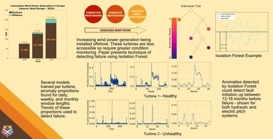
1. Introduction

A significant proportion of the UK energy mix is currently made up of wind energy, both onshore and offshore, and this is only likely to increase. The International Energy Agency’s (IEA) Sustainable Development Scenario [1] predicts that installed offshore wind generation will increase from 19 GW in 2018, to 127 GW in 2040. The IEA have also predicted that the UK’s offshore wind capacity will increase from 8.221 GW in 2018, to 26.9 GW in 2030. With an increase in wind energy generation, the absolute cost and scale of O&M will likely increase with it. The transition from a wind electricity market dominated by onshore turbines to one made up with mostly offshore generation will bring about greater challenges, such as increased downtime and the associated costs.

These costs can be prohibitive to wind farm developers, and the uncertainty around when downtime can occur adds to this. Operations and maintenance (O&M) is an important area of wind energy research. This is due to the previously stated O&M costs, which can be between 20% and 25% of total levelised cost of energy (LCOE) for current wind turbine projects [2], whilst LCOE has been dropping from over $100 per MWh for onshore since 2009 to roughly $50 per MWh in 2019 [3]. The National Renewable Energy Laboratory (NREL) has stated that O&M for U.S. offshore wind energy can cost around £62–187/kW/year [4]. These costs are due in part to the increased failure rate of turbines offshore. On average, these turbines have a failure rate of 10 failures per turbine per year, with 17.5% of these failures being major repairs, and 2.5% being major replacements [5].

The pitch system has one of the highest failure rates of the turbine, but with one of the lowest repair times. This cumulative downtime amounts to roughly 24 thousand euros per MW per year [6]. The ability to schedule maintenance activities around weather and vessel availability would be advantageous and would reduce the offshore wind levelised cost of energy. Due to lower accessibility offshore, a low repair time with a high failure rate can lead to extended downtime. The pitch system, which is referenced as part of the hub in one paper [7], had an average downtime of 0.64 days per year. It has also been stated that the pitch system fails between 0.1 to 0.3 times per year [8]. Each repair offshore will require a sea vessel, with vessel costs making up around 73% of O&M costs offshore [9].

The pitch system is a component in the wind turbine used to regulate power and loads above rated wind speed. This typically consists of an electric, or hydraulic, drive system to rotate the blades over a range of motion as shown in Figure 1, less than a full rotation. As the drive does not continuously rotate, it is difficult to use vibration data for condition monitoring, so SCADA data has become an area of interest. Unlike drivetrain components, high frequency vibration condition monitoring data are unsuitable. Therefore, a technique that can be implemented quickly using SCADA data for wind turbine pitch systems is essential, due to their frequency of failure and their importance to wind turbine power production.

In operational wind farms, wind turbine maintenance practices are typically split into three groups: corrective, scheduled, and condition-based. Corrective maintenance involves performing maintenance action only when the component fails. Scheduled maintenance involves scheduling regular inspections and maintenance actions to monitor the turbine and perform corrective maintenance when necessary. Condition-based maintenance is less common, but becoming more popular in wind energy. This involves actively monitoring turbine components and attempting to predict or detect failures. Once failures are predicted, maintenance action can then be scheduled ahead of time [10].

Anomaly detection is a method of analysis being considered as an efficient and data-driven approach to aid in fault detection. It has been of recent interest due to its ability to detect outliers within data. In past papers, it has been considered as a technique to diagnose or predict faults within components, shown in Section 2. Anomaly detection involves using the data to learn the normal behaviour of the components and then use this to determine anomalous behaviour. It can also be used to estimate turbine health based on this behaviour.

This paper presents a method of condition monitoring using the anomaly detection model of Isolation Forest [11]. An isolation forest is made up of a collection of isolation tree machine learning models (so called because they are based on “decision trees”). These machine learning models are used to learn the normal behaviour of the turbine. Isolation Forest, and anomaly detection in general, is typically an unsupervised training method of machine learning. This is expanded upon more in Section 3.2. The Isolation Forest was trained and tested with Supervisory Control and Data Acquisition (SCADA) data from two different case studies comparing electric and hydraulic pitch systems. Several models were trained per turbine, each trained on a different number of training months. Testing was then conducted for each turbine on a window basis, where the proportion of anomalies within the window was plotted along with previous windows. This systematic testing was carried out to investigate any trend in anomalies in the run-up to failure. This method is presented to allow for fewer data to be stored permanently for active use and can lead to shorter run times. An investigation into the number of training months was carried out, along with the length of the post-processing window used. This method aims to be a tool to assist in the decision-making for scheduling maintenance.

Objectives and Novelty

This paper expands on work presented in [12], which utilised the Isolation Forest model on the turbines with hydraulic pitch systems. The anomaly proportion was only aggregated into monthly windows for post-processing and again analysed to examine the trend. The areas that this paper expands upon are as follows:

• This paper also examines the turbines with electric pitch systems to compare the model effectiveness for different components;
• Examines different aggregate window lengths, these being daily, weekly, and monthly anomaly proportions to assess what window length improves;
• Compares healthy and unhealthy turbine performance, to assess if the model can differentiate.

To the best of the authors’ knowledge, the novelty of this paper is in the use of Isolation Forest to capture daily, weekly, or monthly anomaly proportions over a long period of time. This paper also assesses the number of training months required for the model to be effective—comparing models trained on as little as one month of data. The use of only one month of training data can then improve training times, and could potentially allow turbines with shorter-term historical data to still be effectively monitored. A further novelty is added as the work described above is also the first time anomaly detection techniques have been applied to both hydraulic and electric pitch system condition monitoring for wind turbines.

The objectives of this paper are to provide a useful condition monitoring technique to assist in detecting failures for wind turbine pitch systems, whilst using less training data. To achieve this, the paper tests various Isolation Forest models on a number of wind turbines with different pitch systems and analyses the performance. The best model set-up could then be considered in the future for online operation in the industry.

The structure of the paper is as follows. Section 2 reviews previous literature in condition monitoring for wind turbines. Section 3 outlines the method used in this paper along with a description of the data in the case studies considered. Finally, Section 4 presents and discusses the results from the method outlined in Section 3.

2. Literature Review

2.1. Pitch System Condition Monitoring

Nielsen et al. [13] presented a method of modelling pitch motor torque based on an aeroelastic simulation program called PHATAS. This was proven to work well in certain conditions, however, more work was required to detect pitch damage. Kandukuri et al. [14] utilised fast Fourier transform to analyse the frequency of electrical signals from pitch motors, simulated by FAST using the National Renewable Energy Laboratory’s (NREL) 5 MW reference turbine. A 4-kW induction motor is modelled, and the stator phase A current is measured. Some of the faults examined in this paper are detectable by this technique, however, the broken rotor bar failure is not.

Liu Haitao et al. [15] used a Nonlinear State Estimate Technology algorithm to predict variables, and measure the residuals between the actual and predicted targets. It was able to detect failure ahead of time, but it was unclear as to how long. Yang et al. [16] presented a data-driven approach for wind turbine pitch system condition monitoring. This used three feature selection techniques: sequential forward selection, gradient boosted decision trees, and mutual information, to independently select features, and then choose the common top five features among them. A support vector regression model was used to predict a target based on these features and the mean squared error (MSE) was used to measure its performance, with an exponentially weighted moving average used to detect abnormal performance from the residuals. It was found to outperform multiple other models in both prediction in healthy turbines, and anomaly classification. It could detect at least 37 h ahead of SCADA alarms in 8 different fault cases. Zhu et al. [17] use an extended Kalman Filter-based multiple model adaptive estimation system to estimate the states of the system from a turbine model. This was done to detect the specific fault types—to differentiate between an actuator or sensor fault. A bank of extended Kalman Filters are used first to provide individual estimates and residuals. The residuals are used to give a probability, each combined with the respective estimates. Then, these estimates were blended into one. The model performed well on all faults bar the fault associated with pitch actuator 2 caused by an offset of drive-train torque. It was suggested this could be improved by taking into account the new torque reference. Wei et al. [18] used performance curves to detect failures when turbines are in power generation states. A Gaussian mixture model was used for outlier detection, this split the data into faults and performance curves were used to classify faults. Cho et al. [19,20] have produced two papers looking at fault detection for a floating wind turbine pitch system using Kalman Filters. This used the input command to the actuator and the output of the sensor as inputs to the Kalman Filter, the residuals were compared and if they exceeded a threshold, then a fault was detected. In their first paper [19], the authors then isolated the fault being the cause of the sensor or the actuator through analysing the Nacelle Yaw. In the second paper [20], the fault was diagnosed with an Artificial Neural Network, to differentiate between 6 different fault cases. A paper from He et al. [21] used electrical signature analysis of the pitch system to detect faults. This examined four fault indicators (FI): Negative Sequence FI, Positive Sequence FI, AC ripple peak, and root mean square (RMS). However, there was no indication as to how early this could detect failure. Another paper from Kandukuri et al. [22] presented the use of extended Park vector modulus (EVPM) to detect failures in the pitch system. The EVPM measures energies of specific frequency bands related to known faults, which are then compared to a threshold. If a fault is detected then the energies, plus other time and frequency domain features, are fed into a support vector machine to classify these into faults. This technique could classify faults with an overall accuracy of 98.1%, however would occasionally struggle with a bearing fault. Yang et al. [23] produced another paper for pitch system condition monitoring, using a random forest regression model on SCADA data to detect failure. A relief network was used initially to select 4 features from a set of 9 and then fed only healthy examples of these to the random forest to be trained. It predicted a target health indicator feature, and the residuals were used to detect failure. Three cases were examined, one healthy and two faulty. The technique could detect failure ahead of time, and, in the angle encoder case, fault could be detected before the SCADA alarm. In the limit switch failure case, the SCADA alarm did not detect it, but the technique did before failure. Guo et al. [24] presented a method of normal behaviour modelling for pitch system failure detection. The authors used a multivariate Gaussian process to predict power output and it was found to have smaller residuals and MAE compared to both the binned power curve and sixth-order polynomial model. Sequential Probability Ratio Test was used to detect failures in the residuals produced. This paper could also quickly find the location of the fault by comparing component-related SCADA data before and after failure, along with other data from turbines close to the one examined. Wei et al. [25] presented a technique using relevance vector machines to produce probability distributions of pitch motor power based on SCADA data inputs. Anomalous data were determined by confidence bands based on the healthy normal data. It was found that the average lead time before failure was 76 h for the relevance vector machine and outperformed support vector machines and adaptive neuro-fuzzy inference system (ANFIS) in several metrics. Sandoval et al. [26] presented an approach for low speed bearing diagnosis utilising entropy indicators (EIs). This technique was presented to allow for vibration analysis for slower rotating bearings, where vibration analysis has previously been a challenge. Previously classical indicators, such as kurtosis and root mean square of the time domain have been used, but this paper proposed indicators based on the concept of entropy. Four indicators (approximate entropy, dispersion entropy, singular value decomposition entropy, and spectral entropy of the permutation entropy) were utilised. The paper took a vibration signal, divided it into windows and calculated indicators for each. The average of one rotation time by consecutive time series was found then and the set of indicators were classified with a random forest. This method improved on using classical indicators by up to 22%. This was similar to results found for lower rotational speeds. Further study is required for bearings utilised in real wind turbines, and extending this beyond a test rig. This differs from pitch systems, however, as the pitch system never fully rotates as it travels between roughly 0 and 90 degrees.

2.2. Anomaly Detection for Wind Turbines

Anomaly detection is a technique of machine learning that can be used for condition monitoring. Typically, this is carried out in an unsupervised manner, where the “normal” behaviour of the turbine is unknown and the model is left to learn what is normal behaviour. In some cases, the model can be trained in a supervised learning environment, typically these would be regression models where the prediction error is used as a marker for behaviour. As there are not many examples of anomaly detection for pitch systems, this section will examine anomaly detection for other wind turbine components. Machine learning is also utilised outside of wind energy, with a review of these practices being presented by J. Leukel et al. [27], which examined articles that reported the use of Machine LEarning for predicting failures only using real world data. Of the systems examined, some were wind turbines. The number of articles considered were screened down from 1024 to 34 from a thorough search through Scopus. Overall, they found that Random Forest, Support Vector Machines, and Artificial Neural Networks were the most frequently adopted algorithms. PCA and correlation analysis was considered the most popular feature selection technique. The authors stated that the paper was limited by the heterogeneity of the included studies, as the methods of data collection, pre-processing, training, and evaluation were dissimilar, so no direct comparison could be made. Another paper has presented a review of machine learning techniques in another field. S Nasiri et al. [28] examined the ability to predict behaviour of 3D-printed parts. Machine learning can be used in all aspects of additive manufacturing, from design to evaluation. This paper focussed on the optimisation of process parameters, prediction of porosity of the material, and defect detection. Process optimisation utilised artificial neural networks most commonly, while a variety of methods were used for porosity prediction. Similarly, a wide variety of techniques were used for defect detection. Some challenges found by the authors relate to wind energy, such as availability of larger datasets, and feature selection, or feature ranking, needs further study. Data pre-processing, either through cleaning or image processing, is also considered a priority for further research, similar for wind energy.

Anomaly detection in wind turbines typically investigates the use of both vibration and SCADA data. Local outlier factor (LOF) has been used by Xu et al. [29] to detect abnormal segments of vibration samples. Principal components were extracted from the time domain, and, then, the LOF was used to determine the abnormality of these segments. The k-nearest neighbours of the LOF were found to be an important parameter here. Test rigs are commonly used in vibration to generate sample data, one paper from Abouel-Seoud [30] examined time domain features from vibration data from a test rig gearbox. Faults were introduced artificially, and one-second measurements were taken six times over seven hours. The trend of time-domain features was examined and the root mean square (RMS) of the signal was found to trend upwards before failure for all cases. Neural networks have also been used in anomaly detection, Huitao et al. [31] utilised a wavelet neural network for a test rig gearbox. The network outputs a range of probabilities and the input data corresponds to a specific fault out of five possible faults. It was shown to perform better than empirical model decomposition (EMD). Simulated turbine models have also been utilised to test condition monitoring techniques. Yu et al. [32] used a 4.8 MW Simulink wind turbine model to test a deep belief network, which is made up of stacked unsupervised restricted Boltzmann machines. The model was used to detect sensor, actuator, and system faults, whilst being compared against multiple models and data-driven techniques. It was found to outperform the other models considered. Long Short-Term Memory Neural Networks (LSTM) have also been used in one paper from Liu et al. [33]. The paper used an auto-encoder, with LSTM hidden layers, to encode and decode input sequences from test rig bearings, and the error of the reconstructed data was used to distinguish healthy and unhealthy components. This was done to detect white etching cracks in bearings, which are an indicator of failure. One paper has looked at the combined use of both SCADA and vibration data, which was used with a hybrid anomaly detection model to detect faults in wind turbine drivetrains. The paper from Turnbull et al. [34] examined two cases, one for a wind turbine gearbox only utilising SCADA data, and one for the wind turbine generator using both SCADA and Vibration data. For the gearbox, a neural network was used to model normal behaviour and the errors were then fed into a one-class support vector machine (OCSVM), and, for the second case, two neural networks were used, one for SCADA and one for vibration. The OCSVM then detected anomalies in the error data, and when plotted over time, it could be seen there was a strong trend upwards before failure.

Some recent examples of fault detection for SCADA data from wind turbines are presented here. One paper from Yan et al. [35] used two back-propagated Neural Networks (BPNNs) for feature selection and anomaly detection, respectively. The anomaly detection was carried out based on the root mean squared error (RMSE) between the real and predicted target for a 1.5 MW wind turbine, which could predict failures 15 days in advance. Zhao et al. [36] presented a technique to detect anomalies and, then based on these found anomalies, predict remaining useful life. Density-Based Spatial Clustering of Applications with Noise (DBSCAN) found the anomaly proportion within the data, and then, a Support Vector Machine (SVM) classified whether these outliers were anomalous or not. An auto-regressive integrated moving average (ARIMA) was then used to predict the remaining useful life, and this was achieved with only a mean relative error of 0.27. Overall, the technique could detect faults ahead of time by 44 days. Pei et al. [37] used K Nearest Neighbours (knn) to detect failures in two turbines up to 6 months before failure occurred. The paper presented an instability factor, which was the sequential difference in distances for each new k. This metric was compared to a threshold to detect the upcoming failure. H. Zhao et al. [38] used a Deep Auto-Encoder to reconstruct SCADA variables for three different turbine faults, which were compared to actual values. The errors from this comparison were measured against a threshold developed with extreme value theory and could detect failure up to 10 h quicker than a conventional neural network model, and had a similar computational time. Two separate papers [39,40] presented the similar use of nonlinear auto-regressive neural networks with exogenous inputs (NARX) for anomaly detection. The NARX models predicted a target feature, and then, the Mahalanobis distance between the actual and predicted value was calculated. A threshold was then determined what was anomalous, and if this was crossed continuously then an alarm was generated. Another paper [41] utilised the same technique, however, the wavelet transform was used to denoise the Mahalanobis distance. For both faults considered, this provided a marked improvement over the raw Mahalanobis distance—increasing fault detection time by months. Sun et al. [42] used a Stacked Denoised Auto-Encoder (SDAE) to extract features and feed this into a Clustering in Quest (CLIQUE) model for anomaly detection. This could classify the found outlier with unsupervised learning, however, knowledge of these outliers were known in advance for validation. Overall, this technique could classify outliers with a 98% classification accuracy, which was comparable to other models examined. Zeng et al. [43] utilised a relevance vector machine to estimate the probability distribution of historical gearbox oil temperature to find confidence intervals of predicted values. This model could track normal behaviour and was found to detect failure 8 days ahead for case study 1, and 7 days ahead for case study 2. Autoencoders are also used frequently in anomaly detection, one paper from Lutz et al. [44] used an autoencoder to reconstruct data and the Mahalanobis distance to judge the reconstruction errors. A threshold was set using the false discovery rate by finding the optimal threshold to minimise this. To detect when a failure has occurred, the data were split into time windows and the number of anomalies when operating mode is normal is counted to give a criticality indicator. Dhiman et al. [45] used a two-step process to develop a method of detecting failure. First, an adaptive threshold was used on training data time sequences to declare anomalous segments after twin support vector machines were used for binary classification of these segments. The model was found to have better accuracy than other methods compared and lower false positive and false negative rate. Ensemble methods have been used in other papers, Moreno et al. [46] utilised an ensemble method combining the outputs of weighted K nearest neighbours (wKNN), Boosted Decision Trees, random undersampling Boosted Trees (RUSBoosted Trees), support vector machine, random forest, and rotation forest, and feeding these outputs into another wKNN model. Both just the wKNN and ensemble wKNN performed best on all metrics for detecting true anomalies.

From the literature review, it can be seen that there have not been many papers to utilise Isolation Forest, or examine the effects of using a post-processing window to analyse the anomalies detected. In particular, neither of these have been investigated for the pitch system, and the varying window length has not been examined for this technique previously.

3. Methodology

The aims of this paper is to apply the same technique to two different case studies, each containing multiple turbines and split into different cases depending on what type of pitch system they use. By examining two different pitch systems, the effectiveness and robustness of the model can be found. If similar results are found for both the hydraulic and electric pitch systems, then the model is fairly robust, and can possibly then be applied to other pitch systems with similar components.

In addition, by comparing the post-processing window length, the anomaly trend can possibly be seen in finer detail and give more information as to when an anomaly has occurred.

3.1. Data

Two case studies were examined within this paper. The case studies consisted of two groups of wind turbines, one with an electric pitch system, and the second with a hydraulic pitch system. From here on, the turbines with the electric pitch system will be referred to as case study 1, and the hydraulic pitch system turbines will be referred to as case study 2. Each turbine had different data recording lengths, ranging from 1 year to just over 2 years. The data provided was from the wind turbine SCADA systems, which record data from multiple components and down-samples them to a frequency of 1 recording every ten minutes. This data is common for wind turbines and is available for both case studies investigated.

3.1.1. Case Study 1

The SCADA data for case study 1 were taken from 10 multi-megawatt turbines from the same farm in South America. These turbines utilised an electric pitch system and failed due to a fault in the pitch bearing. This dataset did contain two healthy turbines, this allowed for the technique to be validated against normal behaviour. The healthy turbines did not fail during the time of recording, whereas for the unhealthy turbines for both cases, the data were cut off at turbine failure.

Many features were provided for this dataset, over 200, many of which were categorical data, all features provided were 10-min averaged SCADA data. Each feature was the mean of the data, unfortunately no other statistical data were provided. Domain knowledge was used to select the features used in this case study. The fault causing the failure of these pitch systems was in the bearing. The industrial partner that provided the data identified one feature that helped identify the fault, which was the feedback current from the pitch system, however, this was not always accessible. To investigate the effect of this feature on the condition monitoring technique, models were trained with and without this feature as an input, then performance was assessed. The input features used to train these models are shown in

Table 1. Table of features for both Case Studies investigated.

Case Study	Features
1	Average Wind Speed	Average Power Output	Blade Pitch Angle	Pitch System Motor Temperature	Pitch System Feedback Current
2	Average Wind Speed	Average Power Output	Average Pitch Angle	Average Hydraulic Pitch System Temperature

. According to the industrial partner who provided the data, the Pitch System Feedback Current could be used to detect failure up to 18 months in advance. This was confirmed with on-site inspections by wind turbine technicians that faults had initiated in the pitch bearings.

3.1.2. Case Study 2

The turbines provided for examination in case study 2 were taken from several wind farms in Europe. There were 5 turbines, all were multi-megawatt ratings.

The features provided for Case Study 2 are shown in

Table 2. Features provided in the data for Case Study 2.

Feature	Avg	Max	Min	STD
Generator Speed	x
Hydraulic Pitch Oil Temperature	x
Nacelle Temperature	x
Wind Speed	x	x	x	x
Absolute Wind Direction	x
Relative Wind Direction	x	x	x	x
Power	x
Pitch Angle	x	x	x	x
Nacelle Direction	x

, however, not all of these were utilised in the training and testing of the model. The features that were chosen were selected based on their relative connection to a fault from a paper on hydraulic pitch system suspension faults [47], which is the fault examined here. The features affected by this fault would be the power, pitch angle, and hydraulic oil temperature, and those features selected are shown in Table 1. A paper from D. Astolfi et al. [48] has highlighted the importance of some currently overlooked features, such as the minimum, maximum, and standard deviation of the variables, instead of just utilising the averages. This would have been useful to compare directly between both case studies, however, these features were not provided by the data-supplier. In future work, if possible, it would be useful to conduct this comparison using the other features available. In the time period examined for each turbine in this case study, no failures were recorded until the end of the datasets provided. The time period examined can be considered “healthy” turbine performance.

3.2. Isolation Forest

The model used in this paper is an Isolation Forest model [11]. This model is based on the decision tree model, an example of this is shown in Figure 2, a classifier type. These can predict labels for data, and in the example of Isolation Forest, these labels would be normal or abnormal data. Decision trees are made up of question nodes, that split data up until all data have an individual “branch” of the tree. These trees can be grouped into random forests, which are initialised randomly, to aggregate the results and make the model more robust.

Isolation Forests partition the data until each datapoint is isolated, with the average path length of the branches is then used as the qualifier, with a threshold being learned to classify the data. If the path length is less than this threshold it is considered an anomaly, as sparser anomalous data should require fewer partitions to separate it from clustered normal data. This threshold is dependant on the height of the tree and the average height of the forest. A score is then given to the data, with values closer to a 1 being an anomaly. The anomaly score is generated by the following equation (taken from [11]),

$$s(x,n)=2^{-\frac{E\left(h\right(x\left)\right)}{c\left(n\right)}},$$

(1)

where $h\left(x\right)$ is the average path length to separate input value x, and $c\left(n\right)$ is the average path length of an unsuccessful search of a Binary Search Tree, given by Equation (2).

$$c\left(n\right)=2H(n-1)-\left(2\right(n-1)/n),$$

(2)

where $H(n-1)$ is the harmonic number and can be estimated using $ln(n-1)+0.5772156649$ (Euler’s constant) and n being the number of instances in the dataset. Again, both equations are taken from [11]. Equation (2) is used because an Isolation Tree is based on the structure of a Binary Search Tree, and the estimation of an average path length is similar to the average path length of an unsuccessful search. The score will tend to 1 when the expected path length for an Isolation Tree instance tends to 0, which indicates an anomaly.

Isolation Forest has been used for pre-processing data cleaning in one paper [49] before power prediction is then carried out with neural networks. The IF detected outliers in the power curve were removed, then, a neural network predicted power output for OREC’s 7MW Levenmouth demonstrator turbine. The cleaning technique was compared to an elliptic envelope method, and was found to be more effective.

Isolation forest has been used in conjunction with a Gaussian Mixture Model (GMM) for detection of anomalous behaviour by Chen et al. [50]. This paper took in SCADA data and used the GMM to cluster data by operating condition. Specific component criticality was found by analysing which particular split in an individual tree gave the anomaly.

One other use of Isolation Forest was presented by the authors of [51], where a comparison was made between Isolation Forest, One-Class Support Vector Machine, and Elliptical Envelope, for a condition monitoring technique for wind turbine SCADA data. That paper examined a novel technique that compared two months of data, separated by a year, for several turbines that failed due to a fault in the gearbox. The authors found that Isolation Forest and OCSVM both performed well.

3.3. Condition Monitoring Technique

The method presented in this paper utilises the Isolation Forest model to collect the aggregated anomaly counts for different window lengths and then assesses the trend over time. For each turbine, seven different models were trained. Each model is trained on a different number of months of training data, ranging from 1 to 6 months, and one model is trained on 12 months. Each model was then tested on a window-to-window basis, with the anomaly proportion for each window being compared over time.

The model for each turbine is trained on 1, 2, 3, 4, 5, 6, or 12 months of data. Each model is then tested on the rest of the data for that turbine on a window-by-window basis, which was a day, week, or month long. The proportion of anomalies per window length is then captured and plotted in a trend with the rest of the windows.

For this method, an anomaly was not just a detection made by the Isolation Forest model, it was only considered an anomaly if there were five consecutive detections [52]. This removes any “normal” anomalies, such as turbulence in the wind or other weather effects. It is believed that these effects would not last for 5 consecutive 10-min periods. This technique is illustrated in Figure 3 and also used in [51]. The number of anomalies detected is less relevant than the proportion of anomalies per window. As the number of data-points in the window changes from window to window, the anomaly number would be inappropriate to use. The overall trend will also be more interesting, with spikes on a certain day, week, or month indicating possibly the initiation of a fault or the run up to failure.

This technique could then be applied in industry for an online application. By storing the first month of data available, initial monitoring can be conducted with further months of data being collected live. The anomaly proportion numbers can then be recorded over the long-term life of the turbine and then assessed to detect faults in the future. A new model would need to be trained for each turbine but, as these can be saved and re-used, the model would only need to be trained once. By using this in conjunction with past knowledge of the turbines, operators can then use this as another source of information about the turbine to then improve their decision making concerning maintenance and routine inspections.

4. Results

4.1. Condition Monitoring Technique

Case Study 1 examines the efficacy of the technique, whilst comparing the effects of window length, turbine health, and use of specific features. The turbines featured in case study 1 utilise an electric pitch system, located in South America. The dataset consists of 10 turbines, 8 of these failed in the time recorded and 2 did not. The healthy turbines are numbered 1 and 4 here. The figures presented show the proportion of anomalies per window length examined, over the period investigated. For example, the proportion of anomalies within the daily window would be the fraction of the timesteps within that day that are anomalous, and this is then plotted against time. Case Study 2 was used to validate this technique on different turbine models in a different continent, and with different pitch system components.

The results presented in this section show the proportion of the window length that is anomalous. Figure 4 illustrates the anomaly trend for weekly window lengths. Turbines 1 and 4 here did not fail within the time recorded, and were considered “healthy”.

When comparing the turbines, two features are important to consider: the position of the consistent peaks, and the magnitude of these peaks. Here, a peak is considered a consistent peak where all models, trained on different lengths of data, agree that there is a peak. For example, this is quite prominent for turbine 2, where the three peaks are consistent in location and magnitude.

For the healthy turbines, it can be seen that there are fewer consistent peaks. This is more obvious for turbine 4, where there are many examples of peaks for only one model and no others. This is also evident in turbine 1, but more so for turbine 4. The peaks line up more for the monthly window lengths. Turbine 1 does have one clear peak in the middle of the data meaning this could be an indication of some anomaly, it is possible that the turbine failed after the end of recording as this fault was common for these turbines.

The other turbines, which were considered “unhealthy” appear to have several consistent peaks between 50 and 75 weeks prior to failure. These could be an indication of fault initiation. It can be seen that the models tend to detect a spike in anomalies both roughly 12–18 months before failure, and in the short period in the run-up to failure. It is also unlikely an effect of the seasonality of the data, as these features are apparent in the test results from models trained on 1 month and 12 months of data. If the seasons were affecting the data, this would be apparent in the model trained on 12 months of data, with a peak in the anomalies detected by models trained on fewer months, and no peak from the model trained on 12 months.

The results are promising, with the peaks being consistent across all models presented. Again, it should be noted, that the peak in turbine 1 of Figure 4, is similar to those noted in other unhealthy turbines. This is possibly an indicator of a failure to come, however, further information of the turbine status is unavailable. This is an example of when this condition monitoring technique would be of most use. In this scenario, when a peak is detected in a turbine, a technician could then be sent to do a physical inspection on the pitch system and assess if a fault has initiated.

From other expert advice, it is apparent that some wind farm operators will run turbines even after certain components have failed, sometimes due to a lack of knowledge about their component’s health. With this advanced warning system, maintenance and inspections can be scheduled ahead of failure. The ability to schedule maintenance is of even greater importance for offshore turbines. The restrictions on when maintenance actions can be undertaken offshore, due to weather windows and vessel availability, means that knowing in advance of a potential component failure can potentially reduce downtime and its associated costs.

The findings of this paper could lead to improvements in wind turbine management, allowing for scheduling of wind turbine maintenance. This method has been shown to give notice of turbine failure between 12 and 18 months ahead. The impact of this would be to allow operators to plan maintenance actions ahead of time, and this is particularly more important when turbines are placed offshore as sea conditions and vessel availability can affect when turbines can be accessed for maintenance. So, if turbine condition is known ahead of time, then these issues can be planned around. Turbine downtime, due to failure and maintenance, and the associated costs of this downtime would be reduced due to this ability to take action before the turbine condition becomes severe. Additionally, turbine replacement component inventory is difficult to plan and varies depending on replacement component demand; therefore, notice of upcoming failure can improve inventory planning leading to reduced downtime and in turn lower O&M costs.

4.2. Comparison of Number of Training Months

The number of months used to train each model was varied, with seven models trained per turbine. The effect of the number of training months is examined in this section. Figure 5 presents the anomaly proportions for turbines 1, 2, and 6 comparing the models trained on 1, 3, 6, and 12 months of data.

From Figure 5, the model trained on 1 month of data for turbine 1 does not seem to detect any anomalies throughout the recorded period, compared to the models trained on 3, 6 and 12 months, which look very similar and seem to have the same scale of anomaly proportion. This is also visible between 6 months and 12 months for turbine 2, however, the anomaly proportions from the model trained on 1 month of data does appear to detect the same two peaks as the models trained on 6 and 12 months. This is again another example of consistent peaks. While the peaks change magnitude from 1 to 12 training months, they still indicate where a period of anomalous behaviour occurred. Similarly, for turbine 6, the general trend of anomalies is similar from 1 to 12 months of training data. This shows the robustness of the model, as it is capable of detecting anomalies in unhealthy turbines with only 1 month of training data. For all turbines, there does not appear to be too much change between models trained on 6 months and models trained on 12 months of data.

The performance of the model while only using 1 month of training data is shown to be as effective as models trained with 12 months of data in the unhealthy turbines. This would then allow for faster model training for owners and operators, and would also allow for lower data storage requirements. This method would also allow for ease of analysis in the industry as weekly anomaly proportions can be easily predicted and stored. By examining multiple models on one graph, as shown in Figure 4, peaks can be more confidently identified as anomalous behaviour if they occur for multiple models at once, which would improve the overall robustness of the technique. Potentially, when applied in an online capacity, only 2–4 models would be needed instead of the 7 used here. In isolation, it appears using either 3 or 6 months is the most effective, and using 12 months may not be required.

4.3. Comparison of Window Length

By varying the length of the post-processing window, the resolution of the data can be changed. This is done to first identify a peak in anomalies, then to increase the resolution to identify the day this occurred. By knowing the date of the peak, the cause of the anomalous behaviour can be found (i.e., if it is due to planned or known changes in behaviour). Figure 6 presents the changing window length for turbines 1 and 2, for models trained on 6 months of data only. The focus is on one model per turbine to highlight the differences caused by changing the window length.

Window length affects the magnitude of the peaks in anomaly proportion, this is shown as the scale of the axes reduces with increasing window length, most likely due to large single day, or week, peaks being averaged with surrounding lower peaks. An example of this can be seen for the first two peaks of turbine 2 in Figure 6, which become progressively smaller with increasing window length. Single peaks can appear for increasing window length due to aggregation of smaller peaks in smaller window lengths, and this can make anomalies more prominent in the case of continuous anomalous behaviour. This is shown in turbine 1, with the continual anomalous behaviour after the major spike around day 500. This progressively becomes one secondary peak in the monthly window data.

It can be seen that regardless of what window length is used, the results are rather similar in terms of peak location and number. The main difference is magnitude. In terms of future use of the technique, a monthly window could be used initially to identify areas of anomalous behaviour, then, a daily window length could be used to pinpoint the exact date for analysis. Using a weekly aggregate in isolation appears to be most appropriate, as this filters out much of the noise from the daily aggregate. A weekly aggregate also allows for greater resolution than the monthly aggregate, and when implemented online, it would allow the user to assess when a fault initiation occurred; however, a daily window length is needed to identify the exact day for fault context.

4.4. Effect of Feedback Current

Figure 4 shows the weekly window length for the turbines in Case Study 1 trained on models that utilised the pitch system feedback current feature. It can be seen, when compared to Figure 7, turbines 1, 3, 6, and 9 are all affected by the inclusion of the additional feature.

The pitch system feedback current was considered as a feature on the advice of the industrial partner that supplied the data. This feature had been used to monitor the turbines previously and had shown promise for predicting failure, however has since been made unavailable to the industrial partner. This section therefore looks at the effect of removing this feature from the set of input features, and examining the results from the models. By removing the feedback current from the input set, whether the model still detects anomalies in the same locations as in Figure 4 can be examined. If the performance of the model is still similar when the feature is removed, then this will help to alleviate any problems caused by being denied access to that feature in the future.

This feature had been found to give notice of failure up to 18 months beforehand, and, subsequently, a technician would be sent to inspect the turbine. It was, therefore, important to show that the model still performed as well when trained without this feature. The results shown in Figure 7 are those from the models trained without the feedback current. It can be seen for the unhealthy turbines that a peak is visible roughly 12–18 months before failure at the end of the period examined. This peak is consistent with the findings of the industrial partner, and therefore shows that the model can be trained with other features and still performs as well as when the feedback current is included. This peak before failure could indicate an upcoming fault in the component, as the industrial partner’s technicians described signs of fault initiation at that time.

One particular result that is unexpected is that for turbine 1 the model trained on 2 months of data appears to have inverse results compared with all other models. It is unclear why this has occurred, potentially it is due to a glitch in the data, as it is unlikely due to some excess of anomalies in the first two months of the data, as can be seen in Figure 7.

4.5. Validation against Case Study 2

Figure 8 shows the results for Case Study 2 with a weekly window. This example presents the models not trained on the hydraulic oil temperature feature. Further results for this case study were presented in [12]. The results presented here are used to validate this technique against other turbines with different pitch system components. As this is a hydraulic pitch system, some of the features and behaviours are different compared to an electric pitch system, so are a perfect case study to examine the robustness of the models.

When compared with the results presented for Case Study 1, it can be seen that there are similarities. These are the peak roughly 10–12 months before failure, with a second rise immediately before failure. This second rise is not as visible in turbine 2; however, there does appear to be a consistent peak right before failure. This is despite the turbines in case study 2 using a hydraulic pitch system and the models being trained on different features. As these features are present in both case studies, featuring data recorded at different times and locations, it is unlikely that this is purely coincidental. This indicates that this condition monitoring technique is detecting actual anomalous behaviour, rather than some random noise in the data. This is encouraging as it means that this technique could potentially be applied to other pitch systems and failure modes.

5. Conclusions

This paper has presented a condition monitoring technique using Isolation Forest to assist in maintenance decision-making. This technique compared multiple models per turbine, each trained on a different number of training months. This was then tested on the remaining time and split into windows of time. In summary, the condition monitoring technique examined here is effective in detecting component failure ahead of time. For both the electric and hydraulic pitch systems considered, the technique performed similarly, detecting a peak roughly 12–18 months before failure, and again immediately before failure. This was observed over all the unhealthy turbines examined, these occurrences were asynchronous and did not occur at the same time for each turbine, therefore, this is unlikely to be a coincidence. Various models and aggregate windows were considered. Seven different models were trained per turbine, each corresponding to a different number of training months in the dataset, and three different windows were used to analyse the results of each model.

It was found that a combination of models was useful, as this could show where the models agreed and therefore was likely seeing some anomalous behaviour. It also showed that for the healthy turbines examined that the models would disagree. Whilst analysing the results from the models, a weekly window was useful for removing much of the noise, whilst still allowing for enough resolution to spot when anomalies occur. Overall, this technique has been shown to help improve the scheduling of planned maintenance activities for wind turbines. It was suggested that combining models was useful, however, fewer models are required than presented in this paper. It was found that the model could distinguish between healthy and unhealthy turbines.

In the future, this technique could then be examined again, however, possibly with the use of other features and data. Some features, such as minimum, maximum, and standard deviation of the blade pitch angle, would be of interest to compare for both systems examined, as suggested in [48]. SCADA alarms, or fault information, for the turbines examined could provide contextual data to the results of the model in the future. The authors of [27] state that a future work should consider the effect of feature selection on machine learning techniques, as this has not adequately been investigated in the past.

References

- Offshore Wind Outlook 2019: World Energy Outlook Special Report. Technical Report. 2019. Available online: https://www.iea.org/reports/offshore-wind-outlook-2019 (accessed on 7 October 2021).
- Costa, Á.M.; Orosa, J.A.; Vergara, D.; Fernández-Arias, P. New tendencies in wind energy operation and maintenance. Appl. Sci. 2021, 11, 1386. [Google Scholar] [CrossRef]
- Ren, Z.; Verma, A.S.; Li, Y.; Teuwen, J.J.; Jiang, Z. Offshore wind turbine operations and maintenance: A state-of-the-art review. Renew. Sustain. Energy Rev. 2021, 144, 110886. [Google Scholar] [CrossRef]
- Stehly, T.; Heimiller, D.; Scott, G. 2016 Cost of Wind Energy Review; Technical Report December; National Renewable Energy Lab.: Golden, CO, USA, 2016. [Google Scholar]
- Carroll, J.; McDonald, A.; McMillan, D. Failure rate, repair time and unscheduled O&M cost analysis of offshore wind turbines. Wind Energy 2016, 19, 1107–1119. [Google Scholar] [CrossRef] [Green Version]
- Rinaldi, G.; Thies, P.R.; Johanning, L. Current Status and Future Trends in the Operation and Maintenance of Offshore Wind Turbines: A Review. Energies 2021, 14, 2484. [Google Scholar] [CrossRef]
- Faulstich, S.; Hahn, B.; Tavner, P. Wind Turbine Downtime and its Importance for Offshore Deployment. Wind Energy 2011, 14, 327–337. [Google Scholar] [CrossRef]
- Pinar Pérez, J.M.; García Márquez, F.P.; Tobias, A.; Papaelias, M. Wind turbine reliability analysis. Renew. Sustain. Energy Rev. 2013, 23, 463–472. [Google Scholar] [CrossRef]
- Dalgic, Y.; Lazakis, I.; Turan, O. Vessel charter rate estimation for offshore wind O&M activities. Int. Marit. Assoc. Mediterr. IMAM 2013, 899–908. [Google Scholar] [CrossRef] [Green Version]
- Nielsen, J.J.; Sørensen, J.D. On risk-based operation and maintenance of offshore wind turbine components. Reliab. Eng. Syst. Saf. 2011, 96, 218–229. [Google Scholar] [CrossRef]
- Liu, F.T.; Ting, K.M. Isolation Forest. In Proceedings of the Eighth IEE International Confrence on Data Mining, Pisa, Italy, 15–19 December 2008. [Google Scholar] [CrossRef]
- Mckinnon, C.; Carroll, J.; Mcdonald, A.; Koukoura, S.; Plumley, C. Investigation of anomaly detection technique for wind turbine pitch systems. In Proceedings of the IET RPG 2020, Dublin, Ireland, 1–2 March 2021. [Google Scholar]
- Nielsen, J.S.; van de Pieterman, R.P.; Sorensen, J.D. Analysis of pitch system data for condition monitoring. Wind Energy 2014, 17, 435–449. [Google Scholar] [CrossRef]
- Kandukuri, S.T.; Huynh, V.K.; Karimi, H.R.; Robbersmyr, K.G. Fault Diagnostics for Electrically Operated Pitch Systems in Offshore Wind Turbines. J. Phys. Conf. Ser. 2016, 753. [Google Scholar] [CrossRef] [Green Version]
- Liu, H.; Hao, X.; Kai, H. Fault identification of new energy based on online monitoring. In Proceedings of the 2016 IEEE Advanced Information Management, Communicates, Electronic and Automation Control Conference, IMCEC 2016, Xi’an, China, 3–5 October 2016; pp. 1275–1278. [Google Scholar] [CrossRef]
- Yang, C.; Qian, Z.; Pei, Y.; Wei, L. A data-driven approach for condition monitoring of wind turbine pitch systems. Energies 2018, 11, 2142. [Google Scholar] [CrossRef] [Green Version]
- Zhu, J.; Ma, K.; Hajizadeh, A.; Soltani, M.; Chen, Z. Fault detection and isolation for wind turbine electric pitch system. In Proceedings of the International Conference on Power Electronics and Drive Systems, Honolulu, HI, USA, 12–15 December 2018; pp. 618–623. [Google Scholar] [CrossRef]
- Wei, L.; Qian, Z.; Yang, C.; Pei, Y. Wind turbine pitch system condition monitoring based on performance curves in multiple states. In Proceedings of the 2018 9th International Renewable Energy Congress, IREC 2018, Hammamet, Tunisia, 20–22 March 2018; pp. 1–6. [Google Scholar] [CrossRef]
- Cho, S.; Gao, Z.; Moan, T. Model-based fault detection, fault isolation and fault-tolerant control of a blade pitch system in floating wind turbines. Renew. Energy 2018, 120, 306–321. [Google Scholar] [CrossRef]
- Cho, S.; Choi, M.; Gao, Z.; Moan, T. Fault detection and diagnosis of a blade pitch system in a floating wind turbine based on Kalman filters and artificial neural networks. Renew. Energy 2021, 169, 1–13. [Google Scholar] [CrossRef]
- He, L.; Hao, L.; Pan, D.; Qiao, W. Detection of single-axis pitch bearing defect in a wind turbine using electrical signature analysis. In Proceedings of the 2019 IEEE International Electric Machines and Drives Conference, IEMDC 2019, San Diego, CA, USA, 12–15 May 2019; pp. 31–36. [Google Scholar] [CrossRef]
- Kandukuri, S.T.; Senanyaka, J.S.L.; Huynh, V.K.; Robbersmyr, K.G. A Two-Stage Fault Detection and Classification Scheme for Electrical Pitch Drives in Offshore Wind Farms Using Support Vector Machine. IEEE Trans. Ind. Appl. 2019, 55, 5109–5118. [Google Scholar] [CrossRef]
- Yang, C.; Qian, Z.; Pei, Y. Condition Monitoring for Wind Turbine Pitch System Using Multi-parameter Health Indicator. In Proceedings of the 2018 International Conference on Power System Technology, POWERCON 2018, Guangzhou, China, 6–8 November 2018; pp. 4820–4825. [Google Scholar] [CrossRef]
- Guo, J.; Wu, J.; Zhang, S.; Long, J.; Chen, W.; Cabrera, D.; Li, C. Generative transfer learning for intelligent fault diagnosis of the wind turbine gearbox. Sensors 2020, 20, 1361. [Google Scholar] [CrossRef] [PubMed] [Green Version]
- Wei, L.; Qian, Z.; Zareipour, H. Fault Detection Based on Optimized. IEEE Trans. Sustain. Energy 2020, 11, 2326–2336. [Google Scholar] [CrossRef]
- Sandoval, D.; Leturiondo, U.; Vidal, Y.; Pozo, F. Entropy indicators: An approach for low-speed bearing diagnosis. Sensors 2021, 21, 849. [Google Scholar] [CrossRef]
- Leukel, J.; González, J.; Riekert, M. Adoption of machine learning technology for failure prediction in industrial maintenance: A systematic review. J. Manuf. Syst. 2021, 61, 87–96. [Google Scholar] [CrossRef]
- Nasiri, S.; Khosravani, M.R. Machine learning in predicting mechanical behavior of additively manufactured parts. J. Mater. Res. Technol. 2021, 14, 1137–1153. [Google Scholar] [CrossRef]
- Xu, X.; Lei, Y.; Zhou, X. A LOF-based method for abnormal segment detection in machinery condition monitoring. In Proceedings of the 2018 Prognostics and System Health Management Conference (PHM-Chongqing), Chongqing, China, 26–28 October 2018; pp. 125–128. [Google Scholar] [CrossRef]
- Abouel-seoud, S.A. Fault detection enhancement in wind turbine planetary gearbox via stationary vibration waveform data. J. Low Freq. Noise Vib. Act. Control 2018, 37, 477–494. [Google Scholar] [CrossRef]
- Huitao, C.; Shuangxi, J.; Xianhui, W.; Zhiyang, W. Fault diagnosis of wind turbine gearbox based on wavelet neural network. J. Low Freq. Noise Vib. Act. Control 2018, 37, 977–986. [Google Scholar] [CrossRef] [Green Version]
- Yu, D.; Chen, Z.M.; Xiahou, K.S.; Li, M.S.; Ji, T.Y.; Wu, Q.H. A radically data-driven method for fault detection and diagnosis in wind turbines. Int. J. Electr. Power Energy Syst. 2018, 99, 577–584. [Google Scholar] [CrossRef]
- Liu, X.; Azzam, B.; Harzendorf, F.; Kolb, J.; Schelenz, R.; Hameyer, K.; Jacobs, G. Early stage white etching crack identification using artificial neural networks. Forsch. Ing. 2021, 85, 153–163. [Google Scholar] [CrossRef]
- Turnbull, A.; Carroll, J.; McDonald, A. Combining SCADA and vibration data into a single anomaly detection model to predict wind turbine component failure. Wind Energy 2021, 24, 197–211. [Google Scholar] [CrossRef]
- Yan, Y.; Li, J.; Gao, D.W. Condition Parameter Modeling for Anomaly Detection in Wind Turbines. Energies 2014, 7, 3104–3120. [Google Scholar] [CrossRef] [Green Version]
- Zhao, Y.; Li, D.; Dong, A.; Lin, J.; Kang, D.; Shang, L. Fault prognosis of wind turbine generator using SCADA data. In Proceedings of the NAPS 2016—48th North American Power Symposium, Denver, CO, USA, 18–20 September 2016; pp. 1–6. [Google Scholar] [CrossRef]
- Pei, Y.; Qian, Z.; Tao, S.; Yu, H. Wind Turbine Condition Monitoring Using SCADA Data and Data Mining Method. In Proceedings of the 2018 International Conference on Power System Technology (POWERCON), Guangzhou, China, 6–8 November 2018; pp. 3760–3764. [Google Scholar]
- Zhao, H.; Liu, H.; Hu, W.; Yan, X. Anomaly detection and fault analysis of wind turbine components based on deep learning network. Renew. Energy 2018, 127, 825–834. [Google Scholar] [CrossRef]
- Bangalore, P.; Letzgus, S.; Karlsson, D.; Patriksson, M. An artificial neural network-based condition monitoring method for wind turbines, with application to the monitoring of the gearbox. Wind Energy 2017, 20, 1421–1438. [Google Scholar] [CrossRef]
- Cui, Y.; Bangalore, P.; Tjernberg, L.B. An anomaly detection approach based on machine learning and scada data for condition monitoring of wind turbines. In Proceedings of the 2018 International Conference on Probabilistic Methods Applied to Power Systems, Boise, ID, USA, 24–28 June 2018; pp. 1–6. [Google Scholar] [CrossRef]
- Cui, Y.; Bangalore, P.; Tjernberg, L.B. An Anomaly Detection Approach Using Wavelet Transform and Artificial Neural Networks for Condition Monitoring of Wind Turbines’ Gearboxes. In Proceedings of the 2018 Power Systems Computation Conference (PSCC), Power Systems Computation Conference, Dublin, Ireland, 11–15 June 2018; pp. 1–7. [Google Scholar]
- Sun, Z.; Sun, H. Stacked Denoising Autoencoder With Density-Grid Based Clustering Method for Detecting Outlier of Wind Turbine Components. IEEE Access 2019, 7, 13078–13091. [Google Scholar] [CrossRef]
- Zeng, X.J.; Yang, M.; Bo, Y.F. Gearbox oil temperature anomaly detection for wind turbine based on sparse Bayesian probability estimation. Int. J. Electr. Power Energy Syst. 2020, 123. [Google Scholar] [CrossRef]
- Lutz, M.A.; Vogt, S.; Berkhout, V.; Faulstich, S.; Dienst, S.; Steinmetz, U.; Gück, C.; Ortega, A. Evaluation of anomaly detection of an autoencoder based on maintenace information and SCADA-data. Energies 2020, 13, 1063. [Google Scholar] [CrossRef] [Green Version]
- Dhiman, H.S.; Deb, D.; Muyeen, S.M.; Kamwa, I. Wind Turbine Gearbox Anomaly Detection based on Adaptive Threshold and Twin Support Vector Machines. IEEE Trans. Energy Convers. 2021, 8969, 1–8. [Google Scholar] [CrossRef]
- Moreno, S.R.; Coelho, L.D.S.; Ayala, H.V.; Mariani, V.C. Wind turbines anomaly detection based on power curves and ensemble learning. IET Renew. Power Gener. 2020, 14, 4086–4093. [Google Scholar] [CrossRef]
- Skrimpas, G.A.; Marhadi, K.S.; Gomez, R.; Sweeney, C.W.; Jensen, B.B.; Mijatovic, N.; Holboell, J. Detection of pitch failures in wind turbines using environmental noise recognition techniques. In Proceedings of the Annual Conference of the Prognostics and Health Management Society, PHM, Coronado, CA, USA, 18–24 October 2015; pp. 280–287. [Google Scholar]
- Astolfi, D.; Castellani, F.; Lombardi, A.; Terzi, L. Multivariate SCADA Data Analysis Methods for Real-World Wind Turbine Power Curve Monitoring. Energies 2021, 14, 1105. [Google Scholar] [CrossRef]
- Lin, Z.; Liu, X.; Collu, M. Electrical Power and Energy Systems Wind power prediction based on high-frequency SCADA data along with isolation forest and deep learning neural networks. Electr. Power Energy Syst. 2020, 118, 105835. [Google Scholar] [CrossRef]
- Chen, H.; Ma, H.; Chu, X.; Xue, D. Anomaly detection and critical attributes identification for products with multiple operating conditions based on isolation forest. Adv. Eng. Inform. 2020, 46, 101139. [Google Scholar] [CrossRef]
- McKinnon, C.; Carroll, J.; McDonald, A.; Koukoura, S.; Infield, D.; Soraghan, C. Comparison of new anomaly detection technique for wind turbine condition monitoring using gearbox SCADA data. Energies 2020, 13, 5152. [Google Scholar] [CrossRef]
- Gil, A.; Sanz-Bobi, M.A.; Rodríguez-López, M.A. Behavior anomaly indicators based on reference patterns – Application to the gearbox and electrical generator of a wind turbine. Energies 2018, 11, 87. [Google Scholar] [CrossRef] [Green Version]